Haipeng Cai is with University of Southern Mississippi, e-mail: haipeng.cai@eagles.usm.edu. Jian Chen is with University of Southern Mississippi, e-mail: jian.chen@usm.edu. Alexander P. Auchus is with University of Mississippi Medical Center, e-mail: aauchus@umc.edu. \shortauthortitleHaipeng Caiet al.: ParaDTI \CCScatlist\CCScatComputer GraphicsI.3.1Parallel processing \CCScatComputer GraphicsI.3.4Graphics Utilities
Introduction
Depth-dependent Parallel Visualization with 3D Stylized Dense Tubes
Abstract
We present a parallel visualization algorithm for the illustrative rendering of depth-dependent stylized dense tube data at interactive frame rates. While this computation could be efficiently performed on a GPU device, we target a parallel framework to enable it to be efficiently running on an ordinary multi-core CPU platform which is much more available than GPUs for common users. Our approach is to map the depth information in each tube onto each of the visual dimensions of shape, color, texture, value, and size on the basis of Bertin’s semiology theory. The purpose is to enable more legible displays in the dense tube environments. A major contribution of our work is an efficient and effective parallel depth-ordering algorithm that makes use of the message passing interface (MPI) with VTK. We evaluated our framework with visualizations of depth-stylized tubes derived from 3D diffusion tensor MRI data by comparing its efficiency with several other alternative parallelization platforms running the same computations. As our results show, the parallelization framework we proposed can efficiently render highly dense 3D data sets like the tube data and thus is useful as a complement to parallel visualization environments that rely on GPUs.
keywords
Parallel visualization, stylized rendering, MPI, dense data, MRIWhen visualizing large-scale geometrical data such as dense tubes, one of the critical issues is the visual perception in the depth dimension due to inherent clutters or occlusions as the result of overlapping graphical signs or structures. In order to improve the overall visual legibility from the prospective of depth perception for three-dimension data, mapping depth information to various visual variables of graphical representations can be effective means for enhancing depth perceptions in the dense data visualizations.
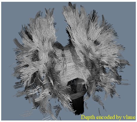
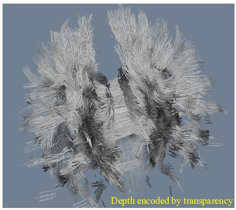
On the basis of Bertin’s semiology theory [10], the primary visual variables to be mapped could include size, color, value and transparency, etc. For instance, a linear mapping from per-vertex depth value to the tube radius (i.e. the size) in the visualization of dense 3D tubes will give viewers a visual cue for discerning depth positions when the radii are gradually decreasing along the viewing direction. Similarly, a consistent mapping from depth to color provides a constant correspondence between distance of geometry and color value thus helps viewers to orient along the depth dimension. In either case, better depth perception is conducive to improvement in overall legibility of the visualized data.
To make the depth-dependent visualizations interactive, real-time computation involved in the depth mappings is required. There are two essential compute-intensive steps to be executed every time the depth reordering is needed, for example when the data view is rotated. First, depth values are calculated according to the updated viewing direction and then sorted along that direction. Second, mappings are computed and then the data are rendered over again to update the visualization. Concisely, depth sorting and re-rendering should be performed once depth order is shuffled as typical result of data transformation that changes the order. In order to obtain an interactive frame rate of such visualizations, therefore, these computations are required to finish in real-time, which have been proven difficult to achieve by our tests, however, with either sequential method or by direct use of currently available facilities such as VTK with its parallelism support.
With this performance challenge, it is reasonable to consider parallelization of the depth-dependent visualization described above to make it interactive. While GPUs are being increasingly applied in many modern parallel computations, and indeed, visualizations of large-scale dense geometry data could be a perfect fit for GPU computing platforms, we aim at a cheaper solution to the same challenges. In particular, we target a solution that can be a useful complement to the GPU computing paradigm when the GPU devices and related high-end hardware configurations are not readily available. In fact, this is mostly true since GPUs are generally much more expensive than ordinary computer users would like to afford for the tasks like the dense tube data visualizations we discuss in this paper, which can indeed be completed with cheap PC hardware using our parallelization framework.
This paper describes a parallel visualization method that supports real-time computations for interactive depth mappings by using the message passing interface (MPI) with VTK while extending current VTK facilities for the purpose of performance optimization. Through the optimized coordination between a parallel depth ordering algorithm and parallel rendering method plus customized data structures for real-time depth mappings, our approach has been verified to be efficient in the visualization scenarios we described by its application to 3D dense tube data.
We have applied the method proposed to depth-dependent 3D dense tube visualizations with depth mappings to all the primary visual variables mentioned before and have obtained interactive rendering speed with either single variable mapping applied or multiple variable mappings freely combined. It is noticeable that even with the combination of mappings from depth to size and those to any other visual variables, in which two passes of depth sorting and rendering plus tube generation from polylines are all required for each frame, our approach has still been able to render the dense data sets at interactive frame rates.
1 Related Work
In this section, we describe previous work most relevant to our parallel visualization method. Related past work can be classified into two categories: depth enhancement and parallel visualization.
1.1 Depth Enhancement
There have been many previous work dedicating to technical solutions to the depth perception issues and visual occlusions in 3D data visualizations. To name a few, a rich set of landmarks and context cues [16] and shading and transparency [9] both contribute in enhancing visual perception in the depth dimension while alleviating occlusion problems within overlapping structures. Focusing on strengthening depth perception, Bruckner et al. employ volumetric halos to improve the 3D legibility of visualized volume data [3]. They introduce different halos according to different ways of halo-volume combination and use halos to construct inconsistent lighting, which accentuates depth even further from another aspect.
Elmqvist et al. [7] give an ever complete discussion about occlusion management in 3D visualization where they focused on reducing 3D occlusions. Occlusion management for visualization is a more general class of visibility problem in computer graphics, which is concerned with improving human perception for specialized visual tasks such as occlusion, size and shape. This method extensively helped improve the legibility of 3D data visualizations. In contrast, we investigate how to manipulate typical retinal variables in graphics perception to help achieve a better depth legibility.
Even direct volume rendering techniques often suffer from poor depth cues because the data sets commonly have a large number of overlapping structures. With MIP (maximum intensity projection) rendering [11], however, only few effort is required to create a good understanding of the structures represented by high signal intensities. This algorithm adds two different visual cues, occlusion revealing and depth based color. In the first one, they modify the MIP color in the presence of occluding objects with the same materials than the one at the point of maximum intensity while in other the actual position of the shaded fragment is used to change its color using a supporting spherical map. In this paper, we explore depth enhancement in dense geometry visualizations by encoding depth information with various visual variables.
Ritter et al. [22] employ hatching strokes to communicate shape while using distance-encoded shadow to further enhance depth perception in their vascular structure visualization. In addition, they achieve a real-time performance using GPU-based hatching algorithm, which is efficient for rendering complex tabular structures with depth being emphasized. Similarly, we handle tabular shapes in our visualization scenario but intend to improve depth perception in a much dense 3D tube geometries derived from human brain MRI data. Also, we we are to provide a cheaper interactive rendering solution on common multi-core CPU than the GPU rendering they have employed.
1.2 Parallel Visualization
Parallelization has been extensively harnessed in visualization scenarios where performance becomes a challenge. In [1], the authors developed a scalable and portable parallel visualization system based on augmenting VTK for efficiently visualizing large scale time-varying data. The system they proposed provides parallelism on both task and pipeline level and primary addressed to visualization programmers. Also at a system scale but even earlier, SCIRun [12] had offered task and data parallelism as a data flow based visualization system running on shared-memory machine with multiprocessors. This system was extended to support task parallelism on distributed-memory architectures [17]. We present a light-weighted parallelization method for large geometry visualization by using existing facilities like MPI and VTK instead of providing a fully featured system or extended programming library.
Compared to the system level solution, a lot more parallelization efforts for visualization focus on parallel rendering, ranging from photo-realistic rendering [21], volume rendering [25] to parallel iso-surfacing [19]. Among a large set of previous work specific to parallel polygon rendering, Crockett [5] harnessed message passing architectures for polygon rendering parallelism that reduces memory usage and network contention while overlapping computation and communication. He also gives an overview of parallel rendering techniques from both hardware and software prospectives later on [4].
Other researchers have probed different indirect aspects, such as image composition schemes [14] and data decomposition strategy [24], to improve polygon rendering performance. More recently, various parallel rendering algorithms including sort-first, sort-last and the hybrid of them, were evaluated when being used on shared-memory computers while these algorithms are originally targeting distributed-memory architectures [18]. In our work, we explore polygon rendering parallelization and employ image compositing as well but particularly serve depth enhancing thus provide a more legible 3D geometry visualization by overlapping parallel depth sorting and parallel polygonal data rendering.
Note that the parallel sorting problem [15, 6], which is at the core of our parallelization framework here, would be easily solved in highly efficient on GPU computing platforms with extensive existing algorithms available [20, 23]. In this paper instead, we target a cheaper solution without relying on high-end computing resources such as GPUs. Alternatively and complementarily, we use CPU-based parallel sorting algorithms leveraging a single processor of multiple cores, which has been almost a bottom-line configuration for modern common computers.
2 Our Methods
2.1 Depth Dimension Management
According to Bertin’s theory, visual legibility of two-dimensional (2D) graphical representations can be characterized by graphical density, angular separation and retinal separation [10]. Further, retinal separation is defined by six visual variables including size, color, shape, value, orientation and texture. Illuminated by the Bertin’s legibility rules described in terms of these dimensions, it is promising to explore the visual legibility issues in 3D data visualizations by examining 3D legibility dimensions. Although, our exploration is still based on the legibility framework proposed by Bertin, certain expansion is required to fully characterize legibility in 3D graphics representations.
While Bertin’s legibility dimensions serve 2D graphical representations, there is a lack of such dimensions for legible 3D data visualizations. We expanded Bertin’s framework from 2D to 3D by adding depth separation dimension that is characteristic of 3D data and examine how typical retinal variables effect legibility of 3D visualizations by investigating visual encodings that map depth information to each one of those variables examined respectively. By such encodings, users are given visual cues to better discern depth locations thus the overall legibility of visualization can be enhanced. Among others, currently we study three variables, size, color and value, which are inherited from Bertin’s framework directly and an extended variable, transparency, which is an important factor influencing depth perception in 3D geometry. In our visual encodings, depth information of geometries can be either encoded by a single visual variable alone or by multiple variables combined. By comparing different encodings, it would be revealed how those visual variables effect the depth separation dimension hence the overall 3D data legibility.
2.2 The Parallel Visualization Pipeline
Our parallel visualization pipeline is outlined in Figure 1. The parallelism is powered by MPI and visualization by VTK with parallelization support. Among the four processes, the master process is responsible for data I/O, visualization interactions and coordinations required for a parallel rendering with consistent depth mappings besides for rendering local data partitions as all other slave processes. The collaborations between the master process and slave processes involve all key steps in the pipeline from data decomposition to parallel depth sorting and geometry rendering.

2.3 Data Decomposition
Data decomposition is ordinarily an essential part for a parallelization mechanism. Although the concrete decomposition scheme can be very much dependent of the interrelations between data components and there are different levels of granularity of the data components as they are defined, it makes sense to split the whole data set into independent partitions as such that data processing of each partition can be performed in parallel. In the case of 3D tubes, for instance, a single tube is regarded as the minimal component and vertices on a tube will not be assigned to different partitions.
In addition, to maximally harness the computing resources available, we decompose the whole geometry model in simply an average manner and then evenly distribute the computational tasks for sorting, mapping and rendering to all processes. This simple data partitioning is efficient for our tube case because for one thing there is no data or semantic dependency among all tubes, and for another, task load for each process is closely equal to others even if the master process will be assigned certain managing roles. However, general data decomposition itself is a separate topic and there is no generally optimal solutions, which are out of the scope of this paper.
When using MPI as the underlying parallel run-time support, the above data are decomposed according to the local process id () and total number of processes specified (). Precisely, given all the data components in the equally-partitioning scheme, local sub-range of data for process will be where . Specially, the last process may take more or less data components than others if is not exactly divided by when . Figure 2 illustrates this data decomposition scheme while showing the overall picture of the depth-stylized visualization is rendered in parallel.
2.4 Parallel Depth Sorting
2.4.1 Per-vertex Depth Ordering
In application scenarios like our 3D stylized dense tube visualization, mappings from depth information of each vertex (or other unit of geometry like triangles or stripes) to visual attributes, such as size, color and transparency that are referred as retinal variables in Bertin’s semiology theory, should be consistent regardless of the current user viewing directions in order to serve depth perception hence visual legibility along the depth dimension of the visualization. In other words, all the vertices (or other geometry units) need to be ordered along the current viewing direction in order to be consistently mapped to visual attribute values. That being said, once the viewing direction changes, typically occurring when users rotate the data view, those vertices need to be reordered before mappings take place over again to refresh the visualization.
In our dense tube environment, vertex-wise depth ordering is required for a depth-dependent tube size assignment with which a better depth perception of even a single 3D tube can be obtained when, for instance, a tube tapers or grows in its radius along the depth direction.
2.4.2 Real Time Sorting
According to the necessity of depth ordering explained above, real-time depth mapping relies on real-time depth sorting. For the per-vertex depth sorting, this computation is essentially the sorting of a sequence of floating-point numbers. For depth sorting of other geometry units, the depth sorting is often eventually reduced to a per-vertex depth sorting problem as well. For instance, if we only want to discern the depth locations at the level of tube rather than that of vertex (thus the visual variable value of vertices on a tube is always the same), a vertex can be selected to represent the tube and then the per-tube sorting is eventually reduced to the depth ordering of the representative vertices.
Therefore, we generalize the depth sorting problem into the sorting of a sequence of cells. Practically, the cell can either be a single value such as floating-point number or a packed data such as a struct including multiple fields. We use the cell array for depth mapping in this paper.
While there are a rich set of parallel sorting algorithms freely available [2], they generally serve the solitary purpose of sorting and are usually implemented as stand-alone parallel applications. Since our ultimate goal is to parallelize dense geometry visualization in which depth mappings are integrated, we need a holistic parallel framework in which the sorting algorithm works together with other steps such as depth mapping and parallel rendering in such a way that the overall visualization performance can be maximized. Our parallel sorting algorithm has been accommodated to parallel rendering (see section 2.5) for which data partitioning is involved, and optimized to mesh with efficient depth mappings (see section 2.6.1).
We adopt mixed sorting algorithm for our parallel depth sorting by the following key steps. Firstly, each process updates the depth values (z-coordinates) of local vertices through a simple vector arithmetic with the current camera parameters (focal point and position, etc). Then, every single process sorts vertex depth values in the partition assigned using a typical quick sort algorithm and sends the sorted depth information to master process once finished. Finally, the master process gathers locally sorted partitions and performs either a multi-way merge sort or multiple two-way merge sort. We employed the latter merge sort scheme on the master process since it is more efficient as an iterative two-way merging can be performed once a sorted partition is received from a slave process without waiting all processes to finish local sorting.
Algorithm 1 shows how this parallel sorting algorithm works while illustrating the real-time depth mappings fit for the parallel visualization framework as a whole.
2.5 Parallel Geometry Rendering
In the application scenarios like our stylized tube visualization, the primary performance challenges come from two sources, namely depth sorting and geometry rendering. For each updated frame, the whole geometry model needs be rendered over again after depth sorting to reflect the depth mapping updates. Although both are critical for a real-time update, the depth sorting time (), compared to the rendering time (), takes only a minor proportion of the whole frame update time ().
According to our sample test with a geometry of 140,000 vertices, is strictly less than in the per-vertex depth-colored visualization. This shows that the rendering part is a bottleneck for the overall visualization performance. In other word, interactive depth-stylized visualization depends on real-time rendering of the depth-mapped geometries. Instead of involving GPU computation that is dependent of graphics hardware architecture, We explore the parallelism in the dense geometry rendering by harnessing multiple computing hardware resource thus provide a cheap yet more readily applicable parallel rendering solution.
Our approach to rendering in parallel is simply consisted of two main steps. After data decomposition, we firstly deploy the local partition to each of the processes. Here a process is a general computing unit that can either be a single processor on multiple-processor platform, a single core on a multi-core processor or a worker thread on a single core processor. For each rendering frame, all separate renditions with each done by a single process are aggregated into a single complete rendition that is only visible on the one of the processes randomly elected as the master process. This aggregation is practically conducted by means of pixel-wise image compositing as the second step detailed as follows.
2.5.1 Pixel-wise Compositing
when each process finished the local rendering of the partition assigned (partial geometry), the rendition is essentially a set of pixels in the frame buffer. As such, pixel-wise compositing is actually a process of compositing frame buffers. In practice, to reduce computational costs, compositing only the color buffer and depth buffer is sufficient for our visualization purpose. For simplicity, we describe compositing with these two types of frame buffer only.
Procedurally, this compositing process is performed by the following three steps: (1) each process fetches pixels from the frame buffers in its local process memory space, and (2) all slave (slave, as opposed to the master) processes send all the buffers one after another to the master process, which do not send its local buffers however. Then, (3) the master process performs a pair-wise buffer compositing every time it receives the buffer from a slave process until all slave buffers are composited. Finally, the master process writes the composited depth and color values back to corresponding local frame buffers as a full image. Figure 2 illustrates this pixel-wise compositing process, an example of which is shown in Figure 3 using 4 processes to parallelize the rendering task.


In addition, when rendering geometries in parallel in the background, the parallelization should be transparent to users. So except for special needs for showing slave renditions, no rendering partitions should be visible and the composited visualization is displayed on the master process only. There are two points to make for the compositing to be optimized.
First, off-screen rendering is applied to avoid slave renditions. This is not only to meet the need of slave renderers for invisible renditions but, more importantly, to improve the overall rendering performance. Second, creation of rendering windows on all slave processes is avoided. Depending on the graphics platform practically used, a less ideal solution is to hide the rendering windows if the creation of them is required for correct rendering. Example case is that a window must be created to establish a context for the drawing to take place. Finally, synchronizing camera parameters across all processes before any process starts to render can simplify the later process of image compositing. As adopted in our approach, a simple way of synchronization is to broadcast the key camera parameters (focal point and position) retrieved on the master process to all slave processes.
2.6 Depth Mappings
Depth mappings are applied to stylize geometry unit according to its depth information so that a better perception in the 3D environment can be obtained. Depending on how the depth value is mapped to the value of different visual variables, a depth mapping is either a linear or non-linear function where is the order of in the sorted sequence and is the depth value of a single geometry unit (vertex will be consistently exemplified in the following text), and function maps the ranking order sequence to the range of designated visual variable, . In the case of linear mapping, for instance,
| (1) |
As we consider size (), color (), value () and transparency () as the variables mapped, is a scalar function. Further, is unitary function for single mapping and multiple mappings are simply an aggregation of multiple single mappings. For example, when mapping depth to size, color and transparency at the same time, is essentially where are all unitary mappings.
2.6.1 Depth Mappings in Parallel Rendering
In the context of geometry rendering, depth mappings are easily performed according to the simple function evaluations as described above. However, depth mappings need be parallelized as well in order to collaborate with parallel rendering towards an optimized performance in the context of visualization parallelization. In our parallel visualization, depth mappings are required to be coherent in the geometry model a whole. Therefore, simply mapping local geometry on each process independently and then compositing the locally depth-stylized renditions do not work.
For each process, the input of depth mapping is the ranking order of depth values of local geometries and, as a result, each process will only have the local rank for every vertex in local its geometry partition. However, the global rank of a vertex in the range of the whole geometry must be retrieved for a coherent global depth mapping. With global ranks of local vertices, every process can render its local geometry independently yet correctly due to the correct mappings from the local vertices to the partition of the range of corresponding to those vertices.
The following figure shows the outline of the integrated parallel sorting and depth mapping algorithm adopted in our parallel visualization.
2.6.2 Hash Index
To figure out the global rank of depth value for each local vertex, reducing all locally sorted partitions together on the master process and then broadcast the resulting depth array that is globally sorted to all other processes can be an easy solution. As such, the global rank will be retrieved from the depth array received for evaluating for each vertex. However, the retrieval would be a search for all local vertices, which is prohibitive enough to make an interactive frame update impossible alone according to our tests. For a real-time global rank retrieval, we create a global hash index for the whole geometry immediately after the depth sort on the master process is all finished.
In both the local and global depth arrays, an index is kept for each depth value at each element and the depth array is actually a sequence of vector where is the depth value and is the index, which is initialized with the original global rank of a vertex in the unsorted holistic geometry. As such, wherever a depth array element is moved after sorting, its original rank, taken as a vertex identifier as well, can be always retrieved immediately. We use this id to associate the unsorted and sorted depth array through the hash index. Figure 4 illustrates the hashing process for depth mapping.

2.6.3 Mapping Update
During the interactive exploration of the depth stylized visualization, mappings need be updated whenever the depth order of geometry along the viewing direction changes, typical because of data rotation. The mapping update is then reflected through refreshed rendering, which is right the reason why we explore the rendering parallelization as discussed before. It is reasonable, therefore, to actively trigger the frame update once mapping update has taken place. There are at least two different mechanisms for the frame update to be timely invoked by mapping updates. First of all, a polygonal data filter, which is used for the purpose of depth sorting, can be inserted into the demand-driven rendering pipeline so that rendering update will be triggered when either the input or output of the filter is modified (using VTK is in this case).
However, besides updating depth mappings, geometry copy between the data filters is required, which has been proven to heavily drag the frame rate. It is noteworthy here that the geometry is not really updated at all when the depth mappings change. Another mechanism is to explicitly invoke frame update (redrawing) through interaction handling. With this approach, only mappings are recomputed while no geometry copying is involved. We employ the latter for a better performance.
In the interaction-driven mapping update mechanism, we only directly handle user input, such as mouse interaction, that shuffles the depth order of geometries on the master process. when responding to such user input, the master process invokes frame update after finishing mapping calculations and then sends a remote method invocation (RMI) message to all slave processes. In the RMI handler on each process, mapping update is firstly triggered, followed by an active call to frame update. Apparently, there is a message processing loop on all processes to enable real-time RMI responding.
3 Implementations
Our parallel depth stylized visualization is implemented in C/C++ using VTK with parallelism support by MPI. In the parallel sorting algorithm, routine from the standard C library for local quick sort on each process and generic in-place merge algorithm in C++ STL library for iterative two-way merge sort on the master process. We have employed the image compositing functionalities provided by VTK’s parallel modules but extended certain classes to tailor their functions for our customized pipeline components in order to implement the pixel-wise compositing. While off-screen rendering has been directly supported in VTK, we make use of wrapping windows by Qt widgets to hide rendering windows of all slave processes.
In addition, our depth sorting filter is extended from VTK’s polygonal data depth sort filter and an interactor component extended from VTK’s track-ball camera interactor, which work together to meet our needs for the interaction-driven mapping update. To explicitly trigger frame update, user-defined RMI messages for this purpose are added and the callbacks are registered to VTK’s multiple process controller component before parallel rendering starts. With these extended components, the interactor responds to data rotation by broadcasting mapping update RMI message to all slave processes and then mapping calculations and frame update are invoked in the callback of the RMI message. The visualization program is simply running as a MPI application and thus the number of processes can be indicated when launching the MPI runtime. As we discuss in detail in section 4, an optimal number of processes to be indicated depends on the actual hardware architecture.
Figure 5 shows the outlook of our test application of the presented parallel visualization method. The GUI framework is created using Qt 4.0 by which all the interaction widgets are set up for the depth stylizing customization. In order to achieve an optimized performance, parallel processing is only applied to the rendering widget and all other GUIs are created on the master process only.
As such, GUI interactions have to be explicitly relayed from the master process where they are triggered to all slave processes so that the slave rendering can reflect the changes in the stylizing configuration as the result of those interactions. We register another type of RMI message and define a dedicated callback to realize the RMI for updating slave renderings. RMI messages are easily transmitted by MPI communications.

4 Results
We have applied the parallel visualization pipeline presented in this paper to interactive depth-stylized visualization for the purpose of investigating legibility issues in 3D data visualizations. As our current application scenarios, we create streamtube visualizations of diffusion tensor MRI (DTI) data with single and multiple depth mappings applied in order to enhance users’ depth perception in the 3D visualizations, as shown in Figure 6.
Also, on the basis of above implementations, we evaluate the efficiency of our parallel visualization approach by firstly measuring the overall rendering performance including depth sorting and MPI communication costs and then comparing our method to other alternative parallel rendering implementations. Our evaluation is based on the results collected from many runs of our test application shown before on a Intel(R) Core(TM)2 Quad 2.66GHz processor with 4GB DDR2 memory.




4.1 Performance Measurements
We measure the proposed parallel visualization method by first comparing visualization performance of the parallel approach to the sequential one with different scales of geometry. Precisely, for each one of the test data sets, the time spent by rendering a single frame in the parallel visualization in milliseconds is paired for comparison with that spent by the same task in sequential one. Here in our application scenarios, we visualize 3D depth stylized streamtubes generated from diffusion tensor MRI data with different depth mapping schemes applied for the tests.
As shown in Figure 7, parallelization enables an interactive rendering performance for our depth-stylized geometry visualization, which is hard to obtain with sequential approach. Each value of the rendering time measurements is an average of the total rendering cost over 100 continuous frames. For the parallel rendering, time measured has included costs of communications among the 4 processes used.

We differentiate only two instances of depth mappings here, depth to color alone and depth to both size and color, because they are representative of two disparate amount of computations for depth mappings in our tests. For the single mapping from depth to color, there is only one round of depth sorting besides the rendering task involved. For the multiple mappings from depth to size and color, there are two rounds of depth sorting plus the tube mesh generation besides rendering task. Among the two rounds of depth sorting, one is for depth of line geometry to size mapping before tubes of different radii are generated and the another for depth of tube geometry to color mapping after tubes are produced from polylines.
To examine how the number of processes used in the parallelization effects the parallel visualization performance, different values of the number has been tested. As the result in Table 1 presents, performance increases monotonically along the increase in the number of processes before the number reaches 4, after which the performance decreases also monotonically when the number continues to grow. That the maximal speedup is achieved at the number of processes of 4 can be attributed to the fact that the number of hard CPU cores is 4.
| Metrics | Number of Processes | |||||
|---|---|---|---|---|---|---|
| 2 | 3 | 4 | 5 | 8 | 12 | |
| Time (ms) | 409 | 359 | 347 | 401 | 469 | 642 |
| Speedup | 1.72 | 1.95 | 2.02 | 1.75 | 1.5 | 1.09 |
| Efficiency | 0.86 | 0.65 | 0.51 | 0.35 | 0.19 | 0.09 |
4.2 Comparisons
we further verify the efficiency of our parallelization approach for depth-stylized geometry rendering by comparing the the overall visualization performance gained by our method with that by other alternative approaches. We implemented the 3D tube visualization with depth-stylizing using both a partially and a fully parallelized rendering. For both comparisons, we gauge the total rendering time with five different scales of 3D tube geometries stylized by depth-dependent color and color, similar to the methodology for measuring performance gain of parallel over sequential visualizations described in section 4.1. Constantly, 4 processes are used in all the following tests.
By comparing to the partially parallel rendering, in which only the depth sorting is parallelized while the overall rendering pipeline is sequential, we intend to show the advantages of our approach with respect to meshing the sorting parallelization with the rendering parallelization. We employed the Kernel for Adaptive, Asynchronous Parallel and Interactive programming (KXAAPI) library [8] to sort the depth information of the whole geometry on the sequential visualization pipeline of VTK. As the results, Figure 8 shows our approach appears much superior and outperforms by more than two folds.

For an alternative fully parallelized visualization solution to compare, we implemented our depth-stylized tube visualization using the IceT module in Paraview [13] with the same measuring method as above. We have partially ported the IceT module from Paraview source package into VTK for the purpose of our test. As is shown in Figure 9, our parallel visualization solution definitely outperforms the IceT based parallelization scheme.

5 Discussion
In our application scenario, we visualize depth-stylized 3D tubes, which is generated in the run-time by wrapping polylines that is loaded into our parallel visualization pipeline. Alternatively, tube meshes can be produced prior to its being loaded to the pipeline then we the computational cost for tube generation will be eliminated. There are two reasons for not doing the off-line tube generation.
First, we need to change the radii of tubes to reflect the depth changes for the depth to size mapping. Loading line geometries and then generating tubes in the run-time is a more efficient way for visualizing tubes with depth to tube size mapping than loading tube meshes directly and then transforming each tube to implement the mapping.
Second, as mentioned in section 4.1, by means of online tube generation, we differentiate two types of mappings, single and multiple, in terms of computational costs in order to demonstrate that a parallel visualization approach like ours will achieve a even superior overall visualization performance if they are more computational steps, such as geometry processing like wrapping poly-lines to produce tube meshes, involved within the whole geometry rendering job.
As a matter of fact, it is obviously shown in the performance measurement results that visualization accelerations are much greater with multiple mappings from depth to size and color than with single mapping from depth to color when the geometry scale is increasing. This is due to that more computations are to be parallelized as well and thus the overall performance gain by parallelization increases compared to sequential visualization. According to this analysis, it is reasonable to scale our parallel visualization method to a more complex visualization context where more compute-intensive steps associated with the rendering task must be involved. Results from our tests before have initially show this type of scalability of our proposed approach.
In addition, although we currently use only a single four-core processor to test our parallelization scheme, it is reasonable to predict that the performance speedup shown in Table 1 will continue to grow if the number of CPU cores further increases. Also, because of the performance scalability of the underlying MPI facilities to processor architecture, application of our method to a multiple processor machine can gain even greater visualization accelerations.
6 Conclusions
We presented a parallel visualization method that enables real-time floating-point computations involved in depth mappings for more legible 3D data visualizations via enhanced depth perception, and therefore helps achieve interactive frame rate in the depth-stylized visualization of large 3D geometries. The method presented is built upon the MPI paradigm within VTK with necessary extension adopted for vertex depth reordering optimizations. Our approach has been tested with 3D dense tubes containing millions of vertices with multiple mappings of depth information applied and the interactive frame rate achieved has shown that our method is efficient for addressing performance issues inherent in the visualization scenarios exemplified in the depth-stylized visualizations. Nevertheless, our method can be easily extended to parallelize visualizations of other large-scale geometry data where intensive computations are required in order to obtain interactive rendering speed.
We have demonstrated the superior efficiency of our approach as a CPU-based parallel visualization framework by comparing the real-time rendering performance of the method presented with that of both sequential method and other parallelization approaches such as XKAAPI and Paraview Icet. As the results show, the proposed framework can provide an efficient alternative to parallel visualization solutions relying on high-end hardware such as GPUs for interactively visualizing large-scale 3D geometry models like stylized dense tubes when the high-end hardware is not readily available.
References
- [1] J. Ahrens, C. Law, W. Schroeder, K. Martin, and M. Papka. A parallel approach for efficiently visualizing extremely large, time-varying datasets. Los Alamos National Laboratory, Los Alamos, New Mexico, Technical Report LAUR-00-1620, 2000.
- [2] G. E. Blelloch. A sampling of parallel sorting algorithms. http://www.cs.cmu.edu/~scandal/nesl/algorithms.html#sort.
- [3] S. Bruckner and E. Gröller. Enhancing depth-perception with flexible volumetric halos. IEEE Transactions on Visualization and Computer Graphics, pages 1344–1351, 2007.
- [4] T. Crockett. An introduction to parallel rendering. Parallel Computing, 23(7):819–843, 1997.
- [5] T. Crockett and T. Orloff. Parallel polygon rendering for message-passing architectures. Parallel & Distributed Technology: Systems & Applications, IEEE, 2(2):17–28, 1994.
- [6] E. K. Donald. The art of computer programming. Sorting and searching, 3:426–458, 1999.
- [7] N. Elmqvist and P. Tsigas. A taxonomy of 3d occlusion management for visualization. IEEE Transactions on Visualization and Computer Graphics, pages 1095–1109, 2008.
- [8] T. Gautier. Kernel for adaptative, asynchronous parallel and interactive programming. http://kaapi.gforge.inria.fr/dokuwiki/doku.php?id=start.
- [9] P. Irani and C. Iturriaga. Labeling nodes in 3d diagrams: Using transparency for text legibility and node visibility. Technical report, University of New Brunswick, 2002.
- [10] B. Jacques. Semiology of graphics: diagrams, networks, maps. University of Wisconsin Press, 1983.
- [11] J.Diaz and P. vazquez. Depth-enhanced maximum intensity projection. International Symposium on Volume Graphics, 8:1–8, 2010.
- [12] C. Johnson and S. Parker. The scirun parallel scientific computing problem solving environment. In Ninth SIAM Conference on Parallel Processing for Scientific Computing, 1999.
- [13] Kitware. Vtk/multipass rendering with icet. http://www.vtk.org/Wiki/VTK/MultiPass_Rendering_With_IceT.
- [14] T. Lee, C. Raghavendra, and J. Nicholas. Image composition schemes for sort-last polygon rendering on 2d mesh multicomputers. IEEE Transactions on Visualization and Computer Graphics, 2(3):202–217, 1996.
- [15] C. E. Leiserson, R. L. Rivest, C. Stein, and T. H. Cormen. Introduction to algorithms. The MIT press, 2001.
- [16] Y. Li, C. Fu, and A. Hanson. Scalable wim: Effective exploration in large-scale astrophysical environments. IEEE Transactions on Visualization and Computer Graphics, pages 1005–1012, 2006.
- [17] M. Miller, C. Hansen, and C. Johnson. Simulation steering with scirun in a distributed environment. Applied Parallel Computing Large Scale Scientific and Industrial Problems, pages 366–376, 1998.
- [18] B. Nouanesengsy, J. P. Ahrens, J. Woodring, and H.-W. Shen. Revisiting parallel rendering for shared memory machines. In EGPGV’11, pages 31–40, 2011.
- [19] S. Parker, P. Shirley, Y. Livnat, C. Hansen, and P. Sloan. Interactive ray tracing for isosurface rendering. In Visualization’98. Proceedings, pages 233–238. IEEE, 1998.
- [20] M. Pharr and R. Fernando. Gpu gems 2: programming techniques for high-performance graphics and general-purpose computation. Addison-Wesley Professional, 2005.
- [21] E. Reinhard, A. Chalmers, and F. Jansen. Overview of parallel photo-realistic graphics. Eurographics’ 98 State of the Art Reports, pages 1–25, 1998.
- [22] F. Ritter, C. Hansen, V. Dicken, O. Konrad, B. Preim, and H. Peitgen. Real-time illustration of vascular structures. Visualization and Computer Graphics, IEEE Transactions on, 12(5):877–884, 2006.
- [23] E. Sintorn and U. Assarsson. Fast parallel gpu-sorting using a hybrid algorithm. Journal of Parallel and Distributed Computing, 68(10):1381–1388, 2008.
- [24] S. Whitman. Dynamic load balancing for parallel polygon rendering. Computer Graphics and Applications, IEEE, 14(4):41–48, 1994.
- [25] C. Wittenbrink. Survey of parallel volume rendering algorithms. Technical report, HEWLETT-PACKARD LABORATORIES, 1998.