Cosmology of Multi-Singlet-Scalar Extensions of the Standard Model Thanks: Presented at the XXXV International Conference of Theoretical Physics ”Matter to the Deepest 2011”

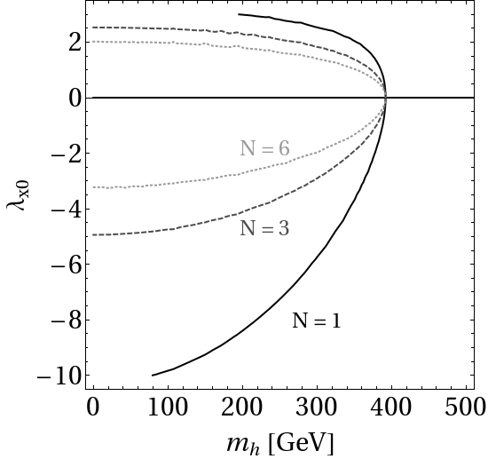
We require that the during the renormalization group equation (RGE) running, the quartic couplings $\lambda_{H},\lambda_{x},\lambda_{\varphi}$ remain finite up to the cut-off scale $\Lambda$. That implies limits on the model parameters, in particular an upper limit on $m_{h}$ (so called ’triviality bound’).

The RGE for running couplings in our model can be found in [6]. We solve those equations with initial conditions: $\lambda_{H}(\mu=m_{W})~=~\lambda_{H\,0}$, $\lambda_{x}(\mu~=~m_{W})~=~\lambda_{x\,0}$ and $\lambda_{\varphi}(\mu=m_{W})=\lambda_{\varphi\,0}$.

We assume that for a given $\Lambda$ there is no pole in the evolution of the scalar quartic couplings at energies below $\Lambda$. That gives us constraints in the $(m_{h},\Lambda)$ plane depending on initial parameters $\lambda_{x\,0},\lambda_{\varphi\,0}$ and $N$ - see the left panel of fig.1. Note that the allowed region shrinks as $\lambda_{x0}$ grows and the upper bound on $m_{h}$ is getting lower. There is also an asymmetry between the negative and positive branch of $\lambda_{x0}$ initial conditions, see the right panel of fig.1

Stability of the singlets $\vec{\varphi}$ makes them good DM candidates. To calculate DM relic abundance in a case of compound DM we need in general a set of Boltzmann equations for all component. Because of the $O(N)$ symmetry it actually simplifies to one equation [8]:

where $f\equiv n/T^{3}$, $n$ is the number density of DM, $f_{EQ}$ is the equilibrium distribution, $g_{\star}(T)$ - number of relativistic degrees of freedom, $m_{Pl}$ - Planck mass, $\left<\sigma v\right>$ - the thermally averaged cross section for $DM+DM\to SM~+~SM$ processes [9], [10]. Total abundance of DM, $\Omega_{\mathrm{DM}}$, reads

where $\Omega_{\mathrm{DM}}^{i}$ is the dark matter relic density from $i$-th scalar field $\varphi_{i}$.

We solve (4) in the standard CDM case [8] using MicrOMEGAs [11]. From the WMAP data [1] we know that $\Omega_{\mathrm{DM}}^{(exp)}h^{2}=0.110\pm 0.018$ (allowing for $3\sigma$ uncertainty) and for a given choice of $N$, $m_{h}$ and $m_{\varphi}$ we seek $\lambda_{x}$ such that this constraint is satisfied, see fig. 2. Note that in the vicinity of resonance, the annihilation cross section is enhanced ($m_{h}\sim 2m_{\varphi}$), therefore $\lambda_{x}$ is suppressed to reach the desired DM abundance.

In the CDM model we achieve equilibrium between certain particles and the SM species just to lose it (’freeze-out’) while the Universe cools. What happens if the DM particles interact with SM so feebly ($\lambda_{x}~<~10^{-9}$), that equilibrium with the SM species is never achieved [12]?

In the following we will assume the number density $f$ was negligible at the Big Bang: $\lim_{T\rightarrow\infty}{f(T)}=0$. Having $f$ determined by the Boltzmann equation (4) (see fig. 3, left panel) one can get the DM relic abundance:

where $T_{\gamma}$ is the present photon temperature, $\rho_{crit}$ is the critical density. For solutions satisfying (6) see fig. 3, right panel.

The direct detection rate of $\vec{\varphi}$ is determined by the cross section of $\vec{\varphi}$ scattering off nuclei (see the Feynman diagram in fig. 4), which can be found e.g. in [9] for $N=1$ and in [7] for compound DM case. In fig. 4 we show allowed regions in the $(m_{h},m_{\varphi})$ plane that remain after imposing limits on the elastic scattering of DM particles off nucleons from XENON100 (the strongest limits on $\sigma_{DM\,N\to DM\,N}$ in the mass range of our interest, [2]). The white band corresponds to the resonance region seen in fig. 2 for $m_{h}\sim 2m_{\varphi}$ in which the annihilation is amplified and the coupling $\lambda_{x}$ is suppressed. Since the XENON100 data start at $m_{\varphi}=5$ GeV therefore the vertical strip of masses below 5 GeV is also allowed.

The standard $\Lambda$CDM model is facing some difficulties if compared with observations. High-resolution N-body simulations have shown that the model generates cusps of the DM density distribution in central regions of galaxies [13] and the number of subhalos predicted by the model turns out to be larger than the observed [14] number. Self-interacting DM (SIDM) was proposed by Spergel & Steinhardt [3] to cure those problems.

The key feature of SIDM is that the mean free path of DM particles should be between 1 kpc and 1 Mpc in regions where the dark matter density is about $0.4\mathrm{\,GeV}/{\mathrm{c}m}^{3}$. In terms of the unit mass cross section the Steinhardt & Spergel hypothesis requires that:

For different $N$ this condition implies a relation between $\lambda_{x},\lambda_{\varphi}$ and $m_{\varphi}$ illustrated in fig. 5 as an allowed region in the ($\lambda_{\varphi},m_{\varphi}$) space. In the plots $\lambda_{\varphi}$ varies form 0 up to its maximal value allowed by unitarity, i.e. $8\pi$. Similar results were obtained in other versions of scalar DM models [15], [16]. As observed from fig. 2, $m_{\varphi}$ consistent with the Spergel and Steinhardt condition is so small that it is not compatible with the CDM case. The only viable option is the FIDM, therefore $\lambda_{x}\sim 0$ (only the first panel in fig. 5 is consistent with the DM abundance). In this case, from fig. 3 one can see that $m_{\varphi}\sim 0.01-0.15$ GeV corresponds to $\lambda_{x}\sim 10^{-10}-10^{-12}$ for $N=1-12$.

References

- [1] N. Jarosik, C. L. Bennett, J. Dunkley, B. Gold, M. R. Greason, M. Halpern, R. S. Hill, G. Hinshaw et al., Astrophys. J. Suppl. 192, 14 (2011). [arXiv:1001.4744 [astro-ph.CO]].
- [2] E. Aprile et al. [XENON100 Collaboration], arXiv:1104.2549 [astro-ph.CO].
- [3] D. N. Spergel, P. J. Steinhardt, Phys. Rev. Lett. 84, 3760-3763 (2000). [astro-ph/9909386].
- [4] B. W. Lee, C. Quigg, H. B. Thacker, Phys. Rev. D16, 1519 (1977).
- [5] G. Cynolter, E. Lendvai, G. Pocsik, Acta Phys. Polon. B36, 827-832 (2005). [hep-ph/0410102]; M. Gonderinger, Y. Li, H. Patel, M. J. Ramsey-Musolf, JHEP 1001, 053 (2010). [arXiv:0910.3167 [hep-ph]].
- [6] Aleksandra Drozd, Master Thesis, not published.
- [7] A. Drozd, B. Grzadkowski and J. Wudka, in preparation.
- [8] E. Kolb, M. Turner, The Early Universe, 1994.
- [9] W. -L. Guo, Y. -L. Wu, JHEP 1010, 083 (2010). [arXiv:1006.2518 [hep-ph]].
- [10] P. Gondolo, G. Gelmini, Nucl. Phys. B360, 145-179 (1991).
- [11] G. Belanger, F. Boudjema, A. Pukhov, A. Semenov, Comput. Phys. Commun. 180, 747-767 (2009). [arXiv:0803.2360 [hep-ph]].
- [12] C. E. Yaguna, JHEP 1108, 060 (2011). [arXiv:1105.1654 [hep-ph]].
- [13] J. F. Navarro, C. S. Frenk, S. D. M. White, Astrophys. J. 490, 493-508 (1997). [astro-ph/9611107].
- [14] A. A. Klypin, A. V. Kravtsov, O. Valenzuela, F. Prada, Astrophys. J. 522, 82-92 (1999). [astro-ph/9901240].
- [15] M. C. Bento, O. Bertolami, R. Rosenfeld, Phys. Lett. B518, 276-281 (2001). [hep-ph/0103340].
- [16] J. McDonald, Phys. Rev. Lett. 88, 091304 (2002). [hep-ph/0106249].