Regional variance for multi-object filteringThanks: Emmanuel D. Delande, Jérémie Houssineau and Daniel E. Clark are with the School of Engineering & Physical Sciences, Heriot-Watt University (HWU), Edinburgh (e-mails: E.D.Delande@hw.ac.uk, jh207@hw.ac.uk and d.e.clark@hw.ac.uk).Thanks: Murat Üney is with the Institute of Digital Communications, University of Edinburgh, Edinburgh (e-mail: M.Uney@ed.ac.uk).

In this article, the objects of interest - the targets - have individual states $x$ in some target space $\mathcal{X}\subset\mathbb{R}^{d_{x}}$, typically consisting of position and velocity variables. The multi-object filtering framework focuses on the target population rather than individual targets. Both the target number and the target states are unknown and (possibly) time-varying. So, we describe the target population by a point process $\Phi$ whose number of elements and element states are random. A realisation of a point process $\Phi$ is a set of points $\varphi=\{x_{1},\dots,x_{N}\}$ depicting a specific multi-target configuration.

More formally, a point process $\Phi$ on $\mathcal{X}$ is a measurable mapping:

from some probability space $(\Omega,\mathcal{F},\mathbb{P})$ to the measurable space $(E_{\mathcal{X}},\mathbf{B}_{E_{\mathcal{X}}})$, where $E_{\mathcal{X}}$ is the point process state space, i.e., the space of all the finite sets of points in $\mathcal{X}$, and $\mathbf{B}_{E_{\mathcal{X}}}$ is the Borel $\sigma$-algebra on $E_{\mathcal{X}}$ [19]. We describe $\Phi$ by its probability distribution on $(E_{\mathcal{X}},\mathbf{B}_{E_{\mathcal{X}}})$ generated by $\mathbb{P}$, denoted by $P_{\Phi}$ (as in the study of random variables). The probability density $p_{\Phi}$ of the point process $\Phi$, if it exists, is the Radon-Nikodym derivative of the probability measure $P_{\Phi}$ with respect to (w.r.t.) the Lebesgue measure.

The Finite Set Statistics methodology for target tracking [6] considers the representation of RFSs through their multi-object density $f_{\Phi}$ (derived from $p_{\Phi}$). This approach has the distinctive merit of producing more intuitive and accessible results facilitating rather direct derivations of filtering algorithms such as the PHD filter [5]. However, the regional variance in target number does not necessarily admit a density, in the general case. Therefore, we chose to adopt a measure-theoretical formulation, based on more general representations of point processes [19], [20], out of practical necessity. A thorough discussion on the relation between measures and associated densities can be found in [21, 22].

Unlike real-valued random variables, the space of point processes is not endowed with an expectation operator from which various statistical moments could be derived. Recall from the definition (1) of a point process $\Phi$ that two realisations $\varphi$, $\varphi^{\prime}\in E_{\mathcal{X}}$ are sets of points. Since the sum of two sets (e.g. $\{x_{1},x_{2}\}+\{x^{\prime}_{1},x^{\prime}_{2},x^{\prime}_{3}\}$) is ill-defined, so would be the “usual” expectation operator $\mathbb{E}[\Phi]$ on point processes.

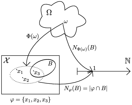
Nevertheless, point processes can alternatively be described by the point patterns they produce in the target state space $\mathcal{X}$ rather than by their realisations in the process state space $E_{\mathcal{X}}$ (see Figure 1). For any Borel set $B\in\mathbf{B}_{\mathcal{X}}$, where $\mathbf{B}_{\mathcal{X}}$ is the Borel $\sigma$-algebra on $\mathcal{X}$, the integer-valued random variable

counts the number of targets falling inside $B$ according to the point process $\Phi$ [19]. Using the well-defined statistical moments of the integer-valued random variables $N_{\Phi}(B)$ for any $B\in\mathbf{B}_{\mathcal{X}}$, one can define the moment measures of the point process $\Phi$.

Note that, $B$ and $B^{\prime}$ can be selected such that they overlap¹¹ 1 In this case, the realisations of $\Phi$ with targets in $B\cap B^{\prime}$ will have non-zero values for both $N_{\Phi}(B)$ and $N_{\Phi}(B^{\prime})$. Consequently, the inner summation in (4c) will have non-zero terms for $i=j$., i.e., $B\cap B^{\prime}\neq\emptyset$. In particular, the variance $\mathrm{var}_{\Phi}$ of the point process $\Phi$ [19] in any region $B\in\mathbf{B}_{\mathcal{X}}$ is defined by

Note that the variance is a function, but not a measure, on the Borel $\sigma$-algebra $\mathbf{B}_{\mathcal{X}}$. It does not necessarily admit a density, in general, even if $\mu^{(2)}_{\Phi}$ and $\mu^{(1)}_{\Phi}$ do. This fact motivates the measure-theoretical approach adopted throughout this article.

Statistical quantities describing a point process can be extracted through differentiation of various functionals, such as its probability generating functional (PGFl) or its Laplace functional (see Section II-D). Several functional differentials may be defined. Moyal used the Gâteaux differential [23] in his early study on point processes [24]; although it is endowed with a sum and a product rule similar to ordinary differentials of real-valued functions, it lacks a chain (or composition) rule that would facilitate the derivation of multi-object filtering equations.

In this article we exploit the multi-object filtering framework in [15, 16], which considers the chain differential [25], in order to prove the results we present in Section III. A restriction of the Gâteaux differential, the chain differential admits a composition rule. The chain differential $\delta F(h;\eta)$ of a functional $F$, (evaluated) at function $h$ in the direction (or increment) $\eta$, is defined as

where $\{\eta_{n}\}_{n\geqslant 0}$ is a sequence of functions $\eta_{n}$ converging (pointwise) to $\eta$, $\{\epsilon_{n}\}_{n\geqslant 0}$ is a sequence of positive real numbers converging to zero, if the limit exists and is identical for any admissible sequences $\{\eta_{n}\}_{n\geqslant 0}$ and $\{\epsilon_{n}\}_{n\geqslant 0}$ [25]. An example of chain differentiation for multi-object filtering is given in [26].

The PGFl of a point process $\Phi$ is defined by the expectation

where $h$ is a test function, i.e., a real-valued function belonging to the space of bounded measurable functions on $\mathcal{X}$, such that $0\leqslant h(x)\leqslant 1$ and $1-h$ vanishes outside some bounded region of $\mathcal{X}$ [20].

The Laplace functional [20, 19] of a point process $\Phi$ is given by the expectation

Both functionals fully characterise the probability distribution $P_{\Phi}$ and are linked by the relation

The probability distribution and the factorial moment measures of a point process can easily be retrieved from functional differentials of the PGFl, making the PGFl a popular tool in multi-object filtering. Mahler’s original construction of the PHD [5] and CPHD [6] filters, for example, exploits the differentiated PGFl. In our derivations for the second-order moment measure, we use non-factorial moment measures which are easily retrieved from the Laplace functional [19]. To be precise, the factorial moment measures $\alpha^{(n)}$ have a different construction and definition than the non-factorial moment measures $\mu^{(n)}$ and will not be considered further in this article with the notable exception of the first factorial moment measure $\alpha^{(1)}$, which coincides with the first (non-factorial) moment measure $\mu^{(1)}$.

In multi-object detection and tracking problems, the target process $\Phi_{k|k}$ is a point process providing a stochastic description of the posterior distribution of the targets in the state space at time $k>0$, based on the measurement history up to time $k$.

Bayesian filtering principles are applicable to the multi-object framework [6]. The law of the filtered state $P_{\Phi_{k|k}}$ is updated through sequences of prediction steps – according (acc.) to target birth, motion, and death models – and data update steps -- acc. to the current set of measurements²² 2 Each measurement has an individual state in the observation space $\mathcal{Z}\subset\mathbb{R}^{d_{z}}$ and $E_{\mathcal{Z}}$ is the space of all the sets of points in $\mathcal{Z}$. $z_{1:m}^{k}\in E_{\mathcal{Z}}$. The full multi-target Bayes’ filter reads as follows [4]:

where $T_{k|k-1}$ is the Markov transition kernel between time steps $k-1$ and $k$, and $L_{k}$ is the multi-measurement/multi-target likelihood at time step $k$ (detailed later)³³ 3 In the scope of this article, the infinitesimal neighbourhoods $dx_{1:n}$ defined around any point $x_{1:n}\in\mathcal{X}^{n}$ are always chosen as elements of the product Borel $\sigma$-algebra $\mathbf{B}_{\mathcal{X}}^{\otimes n}$. Thus, $P(dx_{1:n})=Q(dx_{1:n})$ is a notation for the well-defined expression $\int f(x_{1:n})P(dx_{1:n})=\int f(x_{1:n})Q(dx_{1:n})$ for any test function $f$..

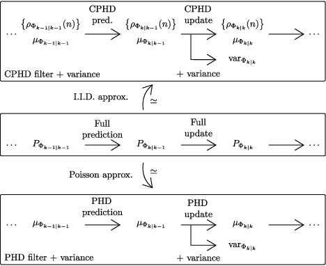
The PHD [5] and the CPHD [6] filters are perhaps the most popular approximations to the multi-target Bayes’ filter (13), (14). The predicted target process $\Phi_{k|k-1}$ is either approximated by an independent and identically distributed (i.i.d.) process (CPHD filter), or by a Poisson process (PHD filter).

An i.i.d. process [29] is completely described by 1) its cardinality distribution $\rho_{\Phi}$⁴⁴ 4 $\rho_{\Phi}(n)$ is the probability that a realisation $\varphi$ of the point process $\Phi$ has size $n$, i.e. the probability that there are exactly $n$ targets in the surveillance scene., and 2) its first moment measure⁵⁵ 5 An i.i.d. process $\Phi$ is usually described by the Radon-Nikodym derivative of its first moment measure $\mu_{\Phi}$ w.r.t. to the Lebesgue measure, also called its first moment density $v_{\Phi}$ or intensity or Probability Hypothesis Density [5]. Since we are interested in producing higher-order statistics on the target number, i.i.d. processes on targets are described by their first moment measure $\mu_{\Phi}$ instead. I.i.d processes on measurements, however, are still described by their intensity $v_{\Phi}$ or, to be precise, by their normalised intensity or spatial distribution (see Theorem 1 and 2). $\mu_{\Phi}$. Hence, the CPHD filter propagates a cardinality distribution $\rho_{\Phi}$ and a moment measure $\mu_{\Phi}$. A Poisson process is a specific case of an i.i.d. process in which the cardinality distribution is a Poisson distribution with rate $\mu_{\Phi}(\mathcal{X})=\int\mu_{\Phi}(dx)$. Hence, a Poisson process is completely described by its first moment measure $\mu_{\Phi}$, propagated by the PHD filter (see Figure 2).

The updated target process $\Phi_{k|k}$ is not, in the general case, i.i.d. (respectively Poisson) even if the predicted $\Phi_{k|k-1}$ is; that is, the updated probability distribution $P_{\Phi_{k|k}}$ is not completely described by the output of the CPHD (respectively PHD) filter. As a consequence, the computation of the variance $\mathrm{var}_{\Phi_{k|k}}$ provides additional information on the updated process $\Phi_{k|k}$, before its collapse into a i.i.d. (respectively Poisson) process in the next time step (see Figure 2).

As shown in Figure 2, this article focuses on the generation of additional information describing the updated target process; hence, the prediction step (15) will not be further mentioned. The rest of the article describes the extraction of the information statistics $(\mu_{\Phi_{k|k}},\mathrm{var}_{\Phi_{k|k}})$ at an arbitrary time step $k>0$. For the sake of simplicity, we discard the time subscripts and denote the predicted and the update processes with $\Phi$ and $\Phi_{+}$ respectively. In addition, we denote the current set of measurements by $z_{1:m}$.

The two following theorems are the main results of this article. Their proof is given in Appendix B (Section B-G).

We consider SMC implementations of the PHD and the CPHD filters and equip them with regional statistiscs. The resulting algorithms are given in Appendix C.

The SMC-PHD filter with regional variance can be easily drawn from the usual SMC-PHD filter [21]. Indeed, the regional variance is computed using the terms that are already computed to find the regional mean (34) in the SMC-PHD filter (see Algorithm 2). The computational complexity of the PHD filter with the variance is still linear w.r.t. the number of current measurements $m$.

Similarly, the construction of the SMC-CPHD filter with regional variance is an extension to the well-known SMC-CPHD filter [29]. As shown in Algorithm 1, the additional corrector terms $\ell_{2}(\phi)$, $\ell_{2}(z)$, and $\ell_{2}(z,z^{\prime})$ (30) are computed in parallel to the usual corrector terms $\ell_{1}(\phi)$ and $\ell_{1}(z)$ (20). In the usual CPHD filter, the bulk of the computational cost stems from the computation of $\ell_{1}(\phi)$ and $\ell_{1}(z)$ in the filtering equation (32) or, more specifically, the elementary symmetric functions (27) appearing in the $\Upsilon^{0}$ and $\Upsilon^{1}$ terms (21). The number of operations to compute $e_{d}(z_{1:m})$ is evaluated at $m\log^{2}m$ in [30] and $m+1$ elementary symmetric functions must be computed for $\ell_{1}(\phi)$ and $\ell_{1}(z)$. Thus, it has been shown by Vo et al. that the computational complexity of the CPHD filter is $\mathcal{O}(m^{2}\log^{2}m)$, where $m$ is the number of current measurements [30].

The corrector terms $\ell_{2}(\phi)$ and $\ell_{2}(z)$ (30), required for the computation of the regional variance (33), do not involve new elementary symmetric functions and can be found in parallel to $\ell_{1}(\phi)$ and $\ell_{1}(z)$ without significant additional cost (see Algorithm 1). On the other hand, $\ell_{2}(z,z^{\prime})$ involves $\frac{m(m-1)}{2}$ different $\Upsilon^{2}$ terms (21) with additional elementary symmetric functions $e_{d}(z,z^{\prime})$ – for every couple of distinct measurements $z,z^{\prime}$. Thus, the computational complexity of the SMC-CPHD filter with regional variance is $\mathcal{O}(m^{3}\log^{2}m)$.

In this example, we consider the regional variance over the FoV under different target detection probabilities. Doing so, we demonstrate the effect of the probability of detection $p_{d}$ on the uncertainty of the estimated target number. We simulate measurements with $p_{d}=0.95,0.90$, and $0.85$ and run both the CPHD and the PHD filters. The mean and the variance in the target number within the FoV (given by the regional statistics evaluated in the whole FoV) are computed using Algorithms 2 and 1.

In Fig. 4–, we present the mean target number in the FoV (blue line) computed using the CPHD filter, together with the ground truth (black line). The variance in target number within the FoV is used to quantify the level of uncertainty in the mean target number. Specifically, we present confidence intervals as the $\pm 1$ square root of the regional variance which in turn admits a standard deviation interpretation. We note that the uncertainty increases as we lower the probability of detection, coinciding with our intuition. The behaviour of the confidence bounds computed using the PHD filter is similar as seen in Fig. 4–.

The regional variances used to find the aforementionned confidence intervals are presented in Fig. 5. In Fig. 5, we plot the results obtained using the CPHD filter as $p_{d}$ goes from $0.95$ to $0.85$. Similar plots for the PHD filter are provided in Fig. 5. The increasing uncertainty with the decreasing $p_{d}$ can clearly be seen. We also note that the variance over the FoV grows significantly more with the PHD than with the CPHD filter as $p_{d}$ is lowered.

In this example, we illustrate the variance evaluated in regions of various sizes within the FoV. Specifically, we consider concentric circular regions of growing radius around the location of target $1$ while its trajectory crosses that of target $2$ (Fig. 6). We vary the radiuses from $r=$1\text{\,}\mathrm{m}$$ to $200\text{\,}\mathrm{m}$ with $1\text{\,}\mathrm{m}$ steps at time steps $t=51,55$ and $59\text{\,}\mathrm{s}$. The distance between the targets are $76.1,5.4$ and $78.9\text{\,}\mathrm{m}$., respectively, at these time instants, so, the regions with larger radius cover both targets.

We compute both the mean target number in these concentric regions and the associated uncertainty quantified by the proposed regional variance. We expect the mean target number to be monotonically increasing as a function of the radius and to reach approximately two for the larger circles. The regional variance, on the other hand, is not necessarily monotonic and we expect its envelope to be an indicator of whether target $1$ can be resolved in the sense that we can identify circular regions that contain only target $1$ with high confidence.

In Fig. 7–, we present the plots of the regional mean and variance in target number (solid black lines) from the CPHD filter as a function of the radius, for a typical run. For $r=$200\text{\,}\mathrm{m}$$, the mean target number in the region is approximately two with very small variance suggesting that with very high confidence, both targets are covered at $t=51,55$ and $59\text{\,}\mathrm{s}$. As the radius increases from $r=$1\text{\,}\mathrm{m}$$ (and the circumferences of the regions depart from target $1$), the uncertainty starts increasing until it reaches a local maximum. The behaviour of the variance curves, after the local maximum and until they reach a small steady value, is of concern. In both Fig. 7 and , the local minimum separating the two maximums clearly indicates that target $1$ is contained with high confidence in a circle whose radius equals the value at the mininum (as the mean target number also reaches one at this minimum). When the targets are located at their closest positions, (Fig. 7), we cannot identify such regions.

We contrast these results with those obtained after filtering the measurements of an inferior range-bearing sensor which has $12.5\text{\,}\mathrm{m}$ and $2.5\text{\,}\mathrm{\SIUnitSymbolDegree}$ standard deviations in range and bearing, respectively. The regional variance for this sensor at $t=51,55$ and $59\text{\,}\mathrm{s}$ (solid red lines in Fig. 7–) stays at a high level until the expected target number reaches two, and, in turn, we are unable to select a region that contains only target $1$ with high confidence. In other words, the two targets are not resolved at these time instants.

In Fig. 7–, we present similar results obtained using the PHD filter. We note that the PHD filter performs as well as the CPHD filter in terms of the ability to resolve the two targets in this particular scenario. As a result, the regional variance computed by any of the filters can effectively be used to assess the level of uncertainty in the estimated number of targets in arbitrary regions.

References

• [1] Y. Bar-Shalom, “ Tracking methods in a multitarget environment,” IEEE T. Automat. Contr., vol. 23, no. 4, pp. 618 – 626, 1978.
• [2] D. Reid, “An Algorithm for Tracking Multiple Targets,” IEEE T. Automat. Contr., vol. 24, no. 6, pp. 843–854, Dec. 1979.
• [3] S. S. Blackman and R. Popoli, Design and analysis of modern tracking systems. Artech House, 1999.
• [4] R. P. S. Mahler, Statistical Multisource-Multitarget Information Fusion. Artech House, 2007.
• [5] ——, “Multitarget Bayes Filtering via First-Order Multitarget Moments,” IEEE T. Aero. Elec. Sys., vol. 39, no. 4, pp. 1152–1178, 2003.
• [6] ——, “PHD Filters of Higher Order in Target Number,” IEEE T. Aero. Elec. Sys., vol. 43, no. 4, pp. 1523–1543, 2007.
• [7] B.-T. Vo and B.-N. Vo, “Labeled Random Finite Sets and Multi-Object Conjuguate Priors,” IEEE T. Signal Proces., vol. 61, pp. 3460 – 3475, 2013.
• [8] M. Üney, D. E. Clark, and S. Julier, “Information Measures in Distributed Multitarget Tracking,” in Information Fusion, Proc. of the 14th International Conference on, 2011, pp. 1 – 8.
• [9] ——, “Distributed Fusion of PHD FIlters via Exponential Mixture Densities,” IEEE J. Sel. Top. Signa., vol. 7, no. 3, pp. 521 – 531, 2013.
• [10] G. Battistelli, L. Chisci, C. Fantacci, A. Farina, and A. Graziano, “Consensus CPHD Filter for Distributed Multitarget Tracking,” IEEE J. Sel. Top. Signa., vol. 7, no. 3, pp. 508 – 520, 2013.
• [11] R. P. S. Mahler, “The multisensor PHD Filter, I: General solution via multitarget calculus,” in Signal Processing, Sensor Fusion, and Target Recognition XVIII, Proc. of SPIE, vol. 7336, 2009.
• [12] E. Delande, E. Duflos, P. Vanheeghe, and D. Heurguier, “Multi-sensor PHD: Construction and implementation by space partitioning,” in Acoustics, Speech and Signal Processing (IEEE ICASSP), 2011.
• [13] B. Ristic and B.-N. Vo, “Sensor Control for Multi-Object State-Space Estimation Using Random Finite Sets,” Automatica, vol. 46, no. 11, pp. 1812–1818, 2010.
• [14] B. Ristic, B.-N. Vo, and D. E. Clark, “A note on the Reward Function for PHD Filters with Sensor Control,” IEEE T. Aero. Elec. Sys., vol. 47, no. 2, pp. 1521–1529, 2011.
• [15] D. E. Clark and J. Houssineau, “Faà di Bruno’s formula for Gâteaux differentials and interacting stochastic population processes,” 2012, arXiv:1202.0264v4.
• [16] ——, “Faà di Bruno’s formula and spatial cluster modelling,” Spatial Statistics, 2013, accepted.
• [17] J. Houssineau, P. Del Moral, and D. E. Clark, “General multi-object filtering and association measure,” in Computational Advances in Multi-Sensor Adaptive Processing (IEEE CAMSAP), 2013.
• [18] S. Singh, B.-N. Vo, A. Baddeley, and S. Zuyev, “Filters for Spatial Point Processes,” SIAM J. Control Optim., vol. 48, no. 4, pp. 2275–2295, 2009.
• [19] D. Stoyan, W. S. Kendall, and J. Mecke, Stochastic geometry and its applications, 2nd ed. Wiley, 1995.
• [20] D. Vere-Jones and D. J. Daley, An Introduction to the Theory of Point Processes, 2nd ed., ser. Statistical Theory and Methods, D. Vere-Jones and D. J. Daley, Eds. Springer Series in Statistics, 2008, vol. 2.
• [21] B.-N. Vo, S. Singh, and A. Doucet, “Sequential Monte Carlo methods for Multi-target Filtering with Random Finite Sets,” IEEE T. Aero. Elec. Sys., vol. 41, no. 4, pp. 1224–1245, 2005.
• [22] J. Houssineau, E. Delande, and D. E. Clark, “Notes of the Summer School on Finite Set Statistics,” 2013, arXiv:1308.2586.
• [23] E. Hille and R. S. Phillips, Functional Analysis and Semi Groups, 2nd ed. American Mathematical Society, 1957.
• [24] J. E. Moyal, “The General Theory of Stochastic Population Processes,” Acta Mathematica, vol. 108, no. 1, pp. 1–31, 1962.
• [25] P. Bernhard, “Chain differentials with an application to the mathematical fear operator,” Nonlinear Analysis, vol. 62, pp. 1225–1233, 2005.
• [26] D. E. Clark and R. P. S. Mahler, “General PHD Filters via a General Chain Rule,” in Information Fusion, Proc. of the 15th International Conference on, 2012.
• [27] E. Delande, J. Houssineau, and D. E. Clark, “PHD filtering with localised target number variance,” in Defense, Security, and Sensing, Proc. of SPIE, 2013.
• [28] ——, “Localised variance in target number for the Cardinalized Hypothesis Density Filter,” in Information Fusion, Proc. of the 16th International Conference on, 2013.
• [29] B.-T. Vo, “Random Finite Sets in Multi-Object Filtering,” Ph.D. dissertation, The University of Western Australia, 2008.
• [30] B.-T. Vo, B.-N. Vo, and A. Cantoni, “Analytic Implementations of the Cardinalized Probability Hypothesis Density Filter,” IEEE T. Signal Proces., vol. 55, pp. 3553–3567, 2007.