跳到论文正文
W Papers独立论文阅读器 arXiv:1310.2516 论文正文 计算阅读时间 · 0%
引用这篇论文根据当前论文元数据生成,正式投稿前建议核对。


License: arXiv.org perpetual non-exclusive license
arXiv:1310.2516v5 [math.NA] 14 Aug 2014

On the backward stability of the second barycentric formula for interpolation

Walter F. Mascarenhas and André Pierro de Camargo ††thanks: Corresponding author. Email: walter.mascarenhas@gmail.com, supported by grant 2013/10916-2 from Fundação de Amparo à Pesquisa do Estado de São Paulo (FAPESP)††thanks: Email: andreuler@yahoo.com.br, supported by grant 14225012012-0 from CNPq Affiliation: Institute of Mathematics and Statistics, Affiliation: University of São Paulo, BRA
Abstract

We present a new stability analysis for the second barycentric formula, showing that this formula is backward stable when the relevant Lebesgue constant is small.

1 Introduction

We discuss the numerical stability of the second barycentric formula for interpolation at nodes x0<x1<…<xnx_{0}<x_{1}<\ldots<x_{n}. This formula is given by

q⁡(x,𝐱,𝐲,𝐰):=∑k=0nwk​ykx−xk/∑k=0nwkx−xk{q}\!\left(x;\mathbf{x},\mathbf{y},\mathbf{w}\right)\ \ :=\ \ \left.\sum\limits_{k=0}^{n}\frac{w_{k}y_{k}}{x-x_{k}}\right/\sum\limits_{k=0}^{n}\frac{w_{k}}{x-x_{k}} (1)

(note that we write the vector 𝐱∈ℝn+1\mathbf{x}\in{\mathds{R}}^{n+1} in bold face, and xkx_{k} is its kkth coordinate.) The function qq may be a polynomial in xx for particular choices of the weights wkw_{k}, but we work in the more general context of rational barycentric interpolation discussed in Berrut (1988),Bos (2012), Bos (2013), Floater (2012) and Hormann (2012).

In practice, we approximate a function f:[x−,x+]→ℝf:[x^{-},x^{+}]\rightarrow\mathds{R}{} using the formula qq in (1) in three steps:

  • Step I:

    Abstract approximation theory provides convenient nodes xkx_{k} and weights wkw_{k}, so that, in exact arithmetic, the error f⁡(x)−q⁡(x,𝐱,f⁡(𝐱),𝐰){f}\!\left(x\right)-{q}\!\left(x;\mathbf{x},{f}\!\left(\mathbf{x}\right),\mathbf{w}\right) is small for x∈[x−,x+]x\in[x^{-},x^{+}].

  • Step II:

    We then obtain floating point approximations x^k\hat{x}_{k}, yky_{k} and w^k\hat{w}_{k} for xkx_{k}, f⁡(xk){f}\!\left(x_{k}\right) and wkw_{k}.

  • Step III:

    Finally, we approximate f⁡(x){f}\!\left(x\right) evaluating q⁡(x,𝐱^,𝐲,𝐰^){q}\!\left(x;\hat{\mathbf{x}},\mathbf{y},\hat{\mathbf{w}}\right) numerically.

This article presents upper and lower bounds on the backward errors in Steps II and III. We also emphasize the importance of considering the errors in these two steps. We focus on the effects of the errors in the nodes 𝐱\mathbf{x} and weights 𝐰\mathbf{w}, and assume that the function values yky_{k} are exact, because perturbations in the function values can be easily handled using Lebesgue constants or by assuming that the perturbed function values are of the form yk​(1+βk)y_{k}\left(1+\beta_{k}\right) with βk\beta_{k} small. We discuss both the case in which the end points of the interval [x−,x+][x^{-},x^{+}] are nodes and the case in which x−x^{-} and x+x^{+} are not nodes, and allow for the possibility that some nodes lie outside of the interval [x−,x+][x^{-},x^{+}].

The overall conclusion is that formula qq in (1) is backward stable when the relevant Lebesgue constant is small, in the sense that the values q⁡(x,𝐱^,𝐲,𝐰^){q}\!\left(x;\hat{\mathbf{x}},\mathbf{y},\hat{\mathbf{w}}\right) obtained numerically in Steps II and III are equal to the exact value q⁡(x~,𝐱,𝐲~,𝐰){q}\!\left(\tilde{x};\mathbf{x},\tilde{\mathbf{y}},\mathbf{w}\right), with x~\tilde{x} near xx and y~k=yk​(1+βk)\tilde{y}_{k}=y_{k}\left(1+\beta_{k}\right) for small βk\beta_{k}s. This conclusion is different from the one presented in Higham (2004), which states that the second barycentric formula is not backward stable. However, there is no contradiction between our conclusion and Higham’s, because we consider the favorable case in which the Lebesgue constant is small and his conclusion applies to the worst possible scenarios.

This article has three more sections. Section 2 presents upper bounds on the backward errors, showing that the second barycentric formula is backward stable under reasonable assumptions. Section 3 gives lower bounds on the backward errors, showing that, for Lagrange polynomials and except for log⁡n\log n factors, the bounds in Section 2 are sharp. The last section contains a perturbation theory for the barycentric formula, which covers the rational as well as the polynomial case. It also presents a proof of the main theorem, which is stated in Section 2.

2 Upper bounds on the backward error

In this section we present upper bounds on the backward errors in the evaluation of the second barycentric formula (1), complementing the bounds presented in Mascarenhas (2014) and Mascarenhas & Camargo (2014). We look at the second formula in (1) as a linear transformation I𝐱,𝐰{\mathrm{I}_{\mathbf{x},\mathbf{w}}} mapping 𝐲∈ℝn+1\mathbf{y}\in{\mathds{R}}^{n+1} to the rational function defined by

I𝐱,𝐰[𝐲](x):={yk​whenx=xk∈{x0,x1,…,xn},∑k=0nwk​ykx−xk/∑k=0nwkx−xk​for​x∈ℝ∖{x0,…,xn}.{\mathrm{I}_{\mathbf{x},\mathbf{w}}\!\left[{\mathbf{y}}\right]}\!\left(x\right):=\ \ \left\{\begin{array}[]{l}y_{k}\ \mathrm{when}\ \ x=x_{k}\in{\left\{x_{0},x_{1},\dots,x_{n}\right\}},\\[5.69046pt] \left.\sum\limits_{k=0}^{n}\frac{w_{k}y_{k}}{x-x_{k}}\right/\sum\limits_{k=0}^{n}\frac{w_{k}}{x-x_{k}}\ \mathrm{for}\ x\in\mathds{R}{}\setminus{\left\{x_{0},\dots,x_{n}\right\}}.\end{array}\right. (2)

The letter I\mathrm{I} in I𝐱,𝐰{\mathrm{I}_{\mathbf{x},\mathbf{w}}} stems from Interpolant, because the function I𝐱,𝐰​[𝐲]:ℝ→ℝ\mathrm{I}_{\mathbf{x},\mathbf{w}}\!\left[{\mathbf{y}}\right]:\mathds{R}{}\rightarrow\mathds{R}{} defined by (2) interpolates the yky_{k} at the xkx_{k}.

The linear map I𝐱,𝐰{\mathrm{I}_{\mathbf{x},\mathbf{w}}} is an abstract way of looking at the second barycentric formula (1), and a practical minded reader can think of I𝐱,𝐰​[𝐲]\mathrm{I}_{\mathbf{x},\mathbf{w}}\!\left[{\mathbf{y}}\right] as a synonym for the function qq in (1). However, by considering the linear map I𝐱,𝐰{\mathrm{I}_{\mathbf{x},\mathbf{w}}} we can think at a deeper level. When the nodes and weights are such that

∑k=0nwkx−xk≠0​for​x∈[x−,x+]∖{x0,…,xn},\sum\limits_{k=0}^{n}\frac{w_{k}}{x-x_{k}}\neq 0\hskip 8.5359pt\mathrm{for}\ x\in[x^{-},x^{+}]\setminus{\left\{x_{0},\dots,x_{n}\right\}}, (3)

the function qq in (1) does not have poles in the interval [x−,x+][x^{-},x^{+}], and I𝐱,𝐰​[𝐲]\mathrm{I}_{\mathbf{x},\mathbf{w}}\!\left[{\mathbf{y}}\right] is an element of the vector space Q⁡(x−,x+)\mathrm{Q}\!\left(x^{-},x^{+}\right) of continuous rational functions from [x−,x+][x^{-},x^{+}] to ℝ\mathds{R}{}, in which we can define the sup norm. It is then natural to study the norm of I𝐱,𝐰{\mathrm{I}_{\mathbf{x},\mathbf{w}}} with respect to the sup norm in ℝn+1{\mathds{R}}^{n+1} and Q⁡(x−,x+)\mathrm{Q}\!\left(x^{-},x^{+}\right). This norm is the Lebesgue constant mentioned in the abstract, and we denote it by Λx−,x+,𝐱,𝐰\Lambda_{x^{-},x^{+},\mathbf{x},\mathbf{w}}. Formally, we define

Λx−,x+,𝐱,𝐰:=‖I𝐱,𝐰‖∞:=supx∈[x−,x+]​and​𝐲≠0|q⁡(x,𝐱,𝐲,𝐰)|‖𝐲‖∞.\Lambda_{x^{-},x^{+},\mathbf{x},\mathbf{w}}:=\left\|{{\mathrm{I}_{\mathbf{x},\mathbf{w}}}}\right\|_{\infty}:=\sup_{x\in[x^{-},x^{+}]\ \mathrm{and}\ \mathbf{y}\neq 0}\frac{\left|{q}\!\left(x;\mathbf{x},\mathbf{y},\mathbf{w}\right)\right|}{\left\|{\mathbf{y}}\right\|_{\infty}}. (4)

The articles Bos (2012), Bos (2013) and Floater (2012) present bounds on these Lebesgue constants, and their bounds allow us to apply the theory developed in Section 4 to the Floater-Hormann interpolants.

Throughout the article we consider a reference interval [x−,x+][x^{-},x^{+}], nodes 𝐱\mathbf{x} and weights 𝐰\mathbf{w}, and perturbed (or rounded) nodes 𝐱^\hat{\mathbf{x}}, with a corresponding interval [x^−,x^+][\hat{x}^{-},\hat{x}^{+}] and weights 𝐰^\hat{\mathbf{w}}. Besides the Lebesgue constant, our analysis of the backward stability of the second barycentric formula is based on the relative errors in the length of the intervals [xj,xk][x_{j},x_{k}], which are measured by

δk​k:=δk​k​(𝐱,𝐱^):=0andδj​k:=δj​k​(𝐱,𝐱^):=xj−xkx^j−x^k−1.\delta_{kk}:={\delta_{kk}}\!\left(\mathbf{x},\hat{\mathbf{x}}\right):=0\hskip 28.45274pt\mathrm{and}\hskip 28.45274pt\delta_{jk}:={\delta_{jk}}\!\left(\mathbf{x},\hat{\mathbf{x}}\right):=\frac{x_{j}-x_{k}}{\hat{x}_{j}-\hat{x}_{k}}-1. (5)

In order to handle rounding errors in the endpoints x−x^{-} and x+x^{+}, and errors in nodes close to them, we also consider

δj−:=δj−​(x−,𝐱,x^−,𝐱^):=x−−xjx^−−x^j−1,\delta^{-}_{j}:={\delta^{-}_{j}}\!\left(x^{-},\mathbf{x},\hat{x}^{-},\hat{\mathbf{x}}\right):=\frac{x^{-}-x_{j}}{\hat{x}^{-}-\hat{x}_{j}}-1, (6)
δj+:=δj+​(𝐱,x+,𝐱^,x^+):=x+−xjx^+−x^j−1,\delta^{+}_{j}:={\delta^{+}_{j}}\!\left(\mathbf{x},x^{+},\hat{\mathbf{x}},\hat{x}^{+}\right):=\frac{x^{+}-x_{j}}{\hat{x}^{+}-\hat{x}_{j}}-1, (7)

with δj−=0\delta^{-}_{j}=0 in the particular case in which x^−=x^j\hat{x}^{-}=\hat{x}_{j}, and δj+=0\delta^{+}_{j}=0 when x^+=x^j\hat{x}^{+}=\hat{x}_{j}. We combine the δj−\delta_{j}^{-}, δj​k\delta_{jk} and δj+\delta_{j}^{+} in the δ\delta given by

δ:=max0≤j,k≤n⁡{|δj−|,|δj​k|,|δj+|}.\delta:=\max_{0\leq j,k\leq n}{\left\{\left|\delta^{-}_{j}\right|,\ \left|\delta_{jk}\right|,\ \left|\delta^{+}_{j}\right|\right\}}. (8)

Another important measure of the perturbations are the relative differences ζk\zeta_{k} between the reference weights 𝐰\mathbf{w} and the weights 𝐰^\hat{\mathbf{w}} used in computation:

ζk:=ζk​(𝐰,𝐰^):=wk−w^kw^k,\zeta_{k}:={\zeta_{k}}\!\left(\mathbf{w},\hat{\mathbf{w}}\right):=\frac{w_{k}-\hat{w}_{k}}{\hat{w}_{k}}, (9)

and to avoid pathological cases we assume that

wk≠0andw^k≠0.w_{k}\neq 0\hskip 28.45274pt\mathrm{and}\hskip 28.45274pt\hat{w}_{k}\neq 0. (10)

We also make the following definitions and assumptions regarding the nodes and endpoints:

xk<xk+1,\displaystyle x_{k}<x_{k+1},\hskip 14.22636pt (11)
xk∈(x−,x+)​if​and​only​if​x^k∈(x^−,x^+),\displaystyle x_{k}\in\left(x^{-},x^{+}\right)\ \mathrm{if\ and\ only\ if}\ \hat{x}_{k}\in\left(\hat{x}^{-},\hat{x}^{+}\right),\hskip 14.22636pt (12)
xk=x−if​and​only​if​x^k=x^−,\displaystyle x_{k}=x^{-}\ \ \mathrm{if\ and\ only\ if}\ \hat{x}_{k}=\hat{x}^{-},\hskip 14.22636pt (13)
xk=x+if​and​only​if​x^k=x^+,\displaystyle x_{k}=x^{+}\ \ \mathrm{if\ and\ only\ if}\ \hat{x}_{k}=\hat{x}^{+},\hskip 14.22636pt (14)
k−​is​the​smallest​k​such​that​xk>x−,\displaystyle k^{-}\ \mathrm{is\ the\ smallest\ }k\ \mathrm{such\ that}\ x_{k}>x^{-},\hskip 14.22636pt (15)
k+​is​the​largest​k​such​that​xk<x+,andk+≥k−.\displaystyle k^{+}\ \mathrm{is\ the\ largest\ }k\ \mathrm{such\ that}\ x_{k}<x^{+},\ \ \mathrm{and}\ \ k^{+}\geq k^{-}.\hskip 14.22636pt (16)

We can now state our main theorem, which provides an upper bound on the backward errors in steps II and III.

Theorem 1.

Under the conditions (3) and (10)–(16), let ϵ\epsilon be the machine precision, assume that (2​n+5)​ϵ<1\left(2n+5\right)\epsilon<1 and define

Z:=‖𝜻⁡(𝐰,𝐰^)‖∞+(n+2)​ϵ1−(n+2)​ϵ.Z:=\frac{\left\|{{\bm{\zeta}}\!\left(\mathbf{w},\hat{\mathbf{w}}\right)}\right\|_{\infty}+\left(n+2\right)\epsilon}{1-\left(n+2\right)\epsilon}. (17)

If, for δ\delta in (8),

(δ+Z)​Λx−,x+,𝐱,𝐰+Z<1,\left(\delta+Z\right)\Lambda_{x^{-},x^{+},\mathbf{x},\mathbf{w}}+Z<1, (18)

and x^∈[x^−,x^+]\hat{x}\in[\hat{x}^{-},\hat{x}^{+}] is a floating point number then the computed value fl⁡(q⁡(x^,𝐱^,𝐲,𝐰^)){\mathrm{fl}}\!\left({q}\!\left(\hat{x};\hat{\mathbf{x}},\mathbf{y},\hat{\mathbf{w}}\right)\right) is equal to q⁡(x,𝐱,𝐲~,𝐰){q}\!\left(x;\mathbf{x},\tilde{\mathbf{y}},\mathbf{w}\right), for some x∈[x−,x+]x\in[x^{-},x^{+}] such that

|x−x^|≤max⁡{‖𝐱−𝐱^‖∞,|x^−−x−|,|x^+−x+|},\left|x-\hat{x}\right|\leq\max{\left\{\left\|{\mathbf{x}-\hat{\mathbf{x}}}\right\|_{\infty},\ \left|\hat{x}^{-}-x^{-}\right|,\ \left|\hat{x}^{+}-x^{+}\right|\right\}}, (19)
y~k=yk​(1+αk)​(1+νk)with‖𝝂‖∞≤(2​n+5)​ϵ1−(2​n+5)​ϵ\tilde{y}_{k}=y_{k}\left(1+\alpha_{k}\right)\left(1+\nu_{k}\right)\hskip 28.45274pt\mathrm{with}\hskip 28.45274pt\left\|{\bm{\nu}}\right\|_{\infty}\leq\frac{\left(2n+5\right)\epsilon}{1-\left(2n+5\right)\epsilon} (20)

and

‖𝜶‖∞≤(1+Λx−,x+,𝐱,𝐰)​(δ+Z)1−Z−(δ+Z)​Λx−,x+,𝐱,𝐰.\left\|{\bm{\alpha}}\right\|_{\infty}\leq\frac{\left(1+\Lambda_{x^{-},x^{+},\mathbf{x},\mathbf{w}}\right)\left(\delta+Z\right)}{1-Z-\left(\delta+Z\right)\Lambda_{x^{-},x^{+},\mathbf{x},\mathbf{w}}}.\\ (21)

Theorem 1 states that the value obtained by the numerical evaluation of the second barycentric formula using approximate nodes 𝐱^\hat{\mathbf{x}} and approximate weights 𝐰^\hat{\mathbf{w}} is the exact value corresponding to 𝐲~\tilde{\mathbf{y}} “near” 𝐲\mathbf{y} and xx “near” x^\hat{x}, according to the measures of nearness in (19)–(21). We emphasize that this theorem takes into account the fact that both the nodes and the weights may have errors in practice, and that by disregarding one of these errors we may underestimate the backward error.

Theorem 1 is abstract and general, and we now present examples of its applicability in concrete situations. We state two corollaries regarding polynomial interpolation at the Chebyshev points of the second kind, which are defined as

xk(c):=−cos⁡(k​π/n),x_{k}^{(c)}:=-{\cos}\!\left(k\pi/n\right), (22)

in combination with weights obtained using the traditional formula

wk=λk​(𝐱):=∏j≠k1xk−xj.w_{k}={\lambda_{k}}\!\left(\mathbf{x}\right):=\prod_{j\neq k}\frac{1}{x_{k}-x_{j}}. (23)

We analyze two scenarios:

  • •

    In the first case we consider weights 𝐰^\hat{\mathbf{w}} given by the closed form expressions in Salzer (1972). These weights are floating point numbers and we call them Salzer’s weights.

  • •

    In the second case we consider the weights obtained by evaluating (23) numerically, using the rounded nodes 𝐱^c:=fl⁡(𝐱c)\hat{\mathbf{x}}^{c}:={\mathrm{fl}}\!\left(\mathbf{x}^{c}\right) and 𝐰^=fl⁡(λ⁡(𝐱^c))\hat{\mathbf{w}}={\mathrm{fl}}\!\left({\lambda}\!\left(\hat{\mathbf{x}}^{c}\right)\right), and we call them Numerical weights.

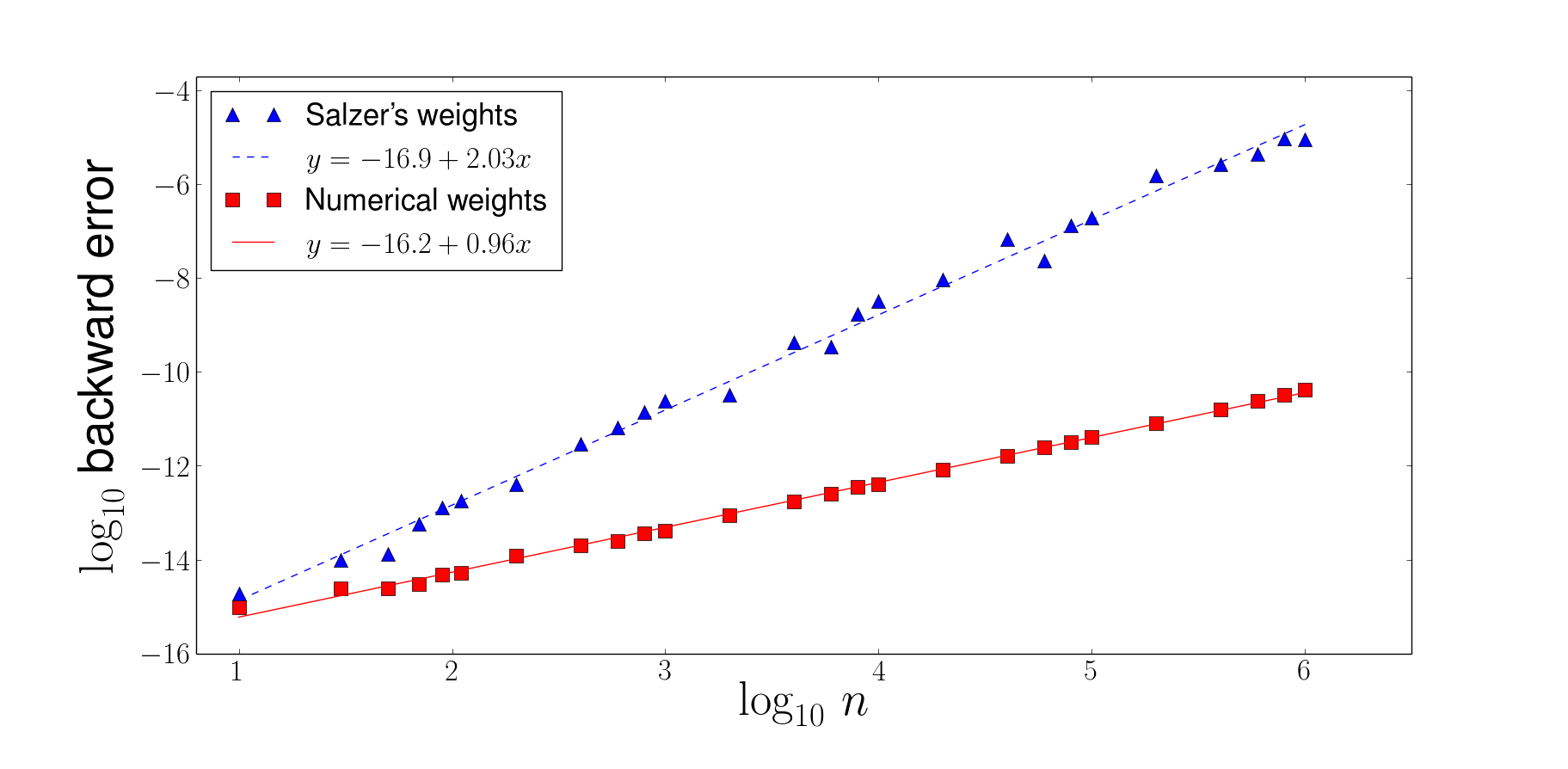
Figure 1 shows that these two cases are quite different for Lagrange polynomials: although Salzer’s weights contain no rounding errors, they lead to much worse results for large nn (the data in this plot comes from Tables 1 and 2 in Section 3.) This difference is also present in Corollaries 1 and 2 below, and by studying their proof the reader will appreciate how Theorem 1 can be applied in practice. Note that these corollaries provide upper bounds on the backward error of order ϵ​n2​log⁡n\epsilon n^{2}\log n for Salzer’s weights and ϵ​n​log⁡n\epsilon n\log n for the Numerical weights, and these numbers are in remarkable agreement with the corresponding lines fitted by the least squares method in Figure 1 (recall that ϵ≈2.3×10⁻¹⁶\epsilon\approx 2.3\times 10^{-16}.)

Refer to caption
Figure 1: The dependency on the weights of the errors with rounded nodes.

We now present our corollaries and their proofs. In the statement of these corollaries, 𝐱c\mathbf{x}^{c} are the Chebyshev nodes in (22), 𝐱^c\hat{\mathbf{x}}^{c} are their rounded counterparts and q⁡(x,𝐱^c,𝐲,λ⁡(𝐱^c)){q}\!\left(x;\hat{\mathbf{x}}^{c},\mathbf{y},{\lambda}\!\left(\hat{\mathbf{x}}^{c}\right)\right) is the nnth degree polynomial that interpolates 𝐲\mathbf{y} at the nodes 𝐱^c\hat{\mathbf{x}}^{c} used in practice.

Corollary 1.

If x^∈[−1,1]\hat{x}\in[-1,1] is a floating point number, 10≤n≤2.000.00010\leq n\leq 2.000.000, ϵ≤2.3×10⁻¹⁶\epsilon\leq 2.3\times 10^{-16}, ‖𝐱^c−𝐱c‖∞≤2​ϵ\left\|{\hat{\mathbf{x}}^{c}-\mathbf{x}^{c}}\right\|_{\infty}\leq 2\epsilon, and 𝐰^s\hat{\mathbf{w}}^{s} are Salzer’s weights, then there exists x∈[−1,1]x\in[-1,1] with |x−x^|≤‖𝐱^c−𝐱c‖∞\left|x-\hat{x}\right|\leq\left\|{\hat{\mathbf{x}}^{c}-\mathbf{x}^{c}}\right\|_{\infty} and 𝛃∈ℝn+1\bm{\beta}\in{\mathds{R}}^{n+1} such that

‖𝜷‖∞≤3.7×(3+log⁡n)​ϵ​n2,\left\|{\bm{\beta}}\right\|_{\infty}\leq 3.7\times\left(3+\log n\right)\epsilon n^{2}, (24)

for which the vector 𝐲~∈ℝn+1\tilde{\mathbf{y}}\in{\mathds{R}}^{n+1} with entries y~k=(1+βk)​yk\tilde{y}_{k}=\left(1+\beta_{k}\right)y_{k} satisfies

fl⁡(q⁡(x^,𝐱^c,𝐲,𝐰^s))=q⁡(x,𝐱^c,𝐲~,λ⁡(𝐱^c)).{\mathrm{fl}}\!\left({q}\!\left(\hat{x};\hat{\mathbf{x}}^{c},\mathbf{y},\hat{\mathbf{w}}^{s}\right)\right)={q}\!\left(x;\hat{\mathbf{x}}^{c},\tilde{\mathbf{y}},{\lambda}\!\left(\hat{\mathbf{x}}^{c}\right)\right).\\ (25)

Proof of Corollary 1. In the context of Corollary 1, the δ\delta in (8) is equal to zero, because we consider the rounded nodes as the interpolation points from the start. When 𝐰=λ⁡(𝐱^c)\mathbf{w}={\lambda}\!\left(\hat{\mathbf{x}}^{c}\right) and 𝐰^=λ⁡(𝐱c)\hat{\mathbf{w}}={\lambda}\!\left(\mathbf{x}^{c}\right), the ζk\zeta_{k} in definition (17) in Mascarenhas & Camargo (2014) is the same as the ζk\zeta_{k} in definition (9) here and Table 2 in that article shows that

‖𝜻‖∞≤2.4624​‖𝐱c−𝐱^c‖∞​n2≤4.9248​ϵ​n2.\left\|{\bm{\zeta}}\right\|_{\infty}\leq 2.4624\left\|{\mathbf{x}^{c}-\hat{\mathbf{x}}^{c}}\right\|_{\infty}n^{2}\leq 4.9248\epsilon n^{2}. (26)

Using that 10≤n≤2×10610\leq n\leq 2\times 10^{6}, we conclude that ZZ in (17) satisfies

Z≤4.9248​ϵ​n2+(n+2)​ϵ1−(2×10⁶+2)×2.3×10−16≤(4.9249​n2+1.0001​n+2.0001)​ϵZ\leq\frac{4.9248\epsilon n^{2}+\left(n+2\right)\epsilon}{1-\left(2\times 10^{6}+2\right)\times 2.3\times 10^{-16}}\leq\left(4.9249n^{2}+1.0001n+2.0001\right)\epsilon
≤(4.9249+1.0001n+2.0001n2)​ϵ​n2≤5.0450​ϵ​n2\leq\left(4.9249+\frac{1.0001}{n}+\frac{2.0001}{n^{2}}\right)\epsilon n^{2}\leq 5.0450\epsilon n^{2}
≤5.0450×4×1012×2.3×10−16≤0.0046414.\leq 5.0450\times 4\times 10^{12}\times 2.3\times 10^{-16}\leq 0.0046414.

Table 2 in Mascarenhas & Camargo (2014) also shows that

Λ−1,1,𝐱^c≤0.67667​log⁡n+1.0236andΛ−1,1,𝐱^c≤10.841,\Lambda_{-1,1,\hat{\mathbf{x}}^{c}}\leq 0.67667\log n+1.0236\hskip 28.45274pt\mathrm{and}\hskip 28.45274pt\Lambda_{-1,1,\hat{\mathbf{x}}^{c}}\leq 10.841,

and it follows that the 𝜶\bm{\alpha} in (20) satisfies

‖𝜶‖∞≤0.67667​log⁡n+2.02361−0.0046414×11.841×5.0450​ϵ​n2≤3.6124​(3+log⁡n)​ϵ​n2.\left\|{\bm{\alpha}}\right\|_{\infty}\leq\frac{0.67667\log n+2.0236}{1-0.0046414\times 11.841}\times 5.0450\epsilon n^{2}\leq 3.6124\left(3+\log n\right)\epsilon n^{2}.

The assumptions on ϵ\epsilon and nn lead to

(2​n+5)​ϵ≤(4×10⁶+5)×2.3×10−16<9.2001×10⁻¹⁰,\left(2n+5\right)\epsilon\leq\left(4\times 10^{6}+5\right)\times 2.3\times 10^{-16}<9.2001\times 10^{-10},

and (20) leads to |ν|k≤1.0001​(2​n+5)​ϵ<9.2011×10⁻¹⁰\left|\nu\right|_{k}\leq 1.0001\left(2n+5\right)\epsilon<9.2011\times 10^{-10}. It follows that βk:=νk+(1+νk)​αk\beta_{k}:=\nu_{k}+\left(1+\nu_{k}\right)\alpha_{k} satisfies

|βk|≤1.0001​(2​n+5)​ϵ+(1+9.2011×10−10)×3.6124​(3+log⁡n)​ϵ​n2\left|\beta_{k}\right|\leq 1.0001\left(2n+5\right)\epsilon+\left(1+9.2011\times 10^{-10}\right)\times 3.6124\left(3+\log n\right)\epsilon n^{2}
≤(1.0001​(2​n+5)3.6124​n2​(3+log⁡n)+1)×3.6124×(3+log⁡n)​ϵ​n2≤3.6597​(3+log⁡n)​ϵ​n2\leq\left(\frac{1.0001\left(2n+5\right)}{3.6124n^{2}\left(3+\log n\right)}+1\right)\times 3.6124\times\left(3+\log n\right)\epsilon n^{2}\leq 3.6597\left(3+\log n\right)\epsilon n^{2}

Therefore, βk\beta_{k} satisfies (24). Theorem 1 yields x^\hat{x} as in (25) and we are done.
∎

Corollary 2.

If x^∈[−1,1]\hat{x}\in[-1,1] is a floating point number, 10≤n≤2.000.00010\leq n\leq 2.000.000, ϵ≤2.3×10⁻¹⁶\epsilon\leq 2.3\times 10^{-16}, ‖𝐱^c−𝐱c‖∞≤2​ϵ\left\|{\hat{\mathbf{x}}^{c}-\mathbf{x}^{c}}\right\|_{\infty}\leq 2\epsilon, and 𝐰^r\hat{\mathbf{w}}^{r} are the Numerical weights fl⁡(λ⁡(𝐱^c)){\mathrm{fl}}\!\left({\lambda}\!\left(\hat{\mathbf{x}}^{c}\right)\right), then there exists x∈[−1,1]x\in[-1,1] with |x−x^|≤‖𝐱^c−𝐱c‖∞\left|x-\hat{x}\right|\leq\left\|{\hat{\mathbf{x}}^{c}-\mathbf{x}^{c}}\right\|_{\infty} and 𝛃∈ℝn+1\bm{\beta}\in{\mathds{R}}^{n+1} such that

‖𝜷‖∞≤(2.2​log⁡n+9.1)​ϵ​n.\left\|{\bm{\beta}}\right\|_{\infty}\leq\left(2.2\log n+9.1\right)\epsilon n. (27)

for which the the vector 𝐲~∈ℝn+1\tilde{\mathbf{y}}\in{\mathds{R}}^{n+1} with entries y~k=(1+βk)​yk\tilde{y}_{k}=\left(1+\beta_{k}\right)y_{k} satisfies

fl⁡(q⁡(x^,𝐱^c,𝐲,𝐰^r))=q⁡(x,𝐱^c,𝐲~,λ⁡(𝐱^c)).{\mathrm{fl}}\!\left({q}\!\left(\hat{x};\hat{\mathbf{x}}^{c},\mathbf{y},\hat{\mathbf{w}}^{r}\right)\right)={q}\!\left(x;\hat{\mathbf{x}}^{c},\tilde{\mathbf{y}},{\lambda}\!\left(\hat{\mathbf{x}}^{c}\right)\right).\\ (28)

Proof of Corollary 2. Lemma 3.1 in Higham (2004) states that

wk(r)=wk​⟨2​n⟩k,w_{k}^{\left(r\right)}=w_{k}\langle{2n}\rangle_{k},

and using Lemma 3.1 in Higham (2002) we conclude that the ζk\zeta_{k} in (9) satisfy

|ζk|=|wk−wk​⟨2​n⟩kwk​⟨2​n⟩k|=|1−⟨2​n⟩k||⟨2​n⟩k|=|⟨2​n⟩k′−1|≤2​ϵ​n1−2​ϵ​n\left|\zeta_{k}\right|=\left|\frac{w_{k}-w_{k}\langle{2n}\rangle_{k}}{w_{k}\langle{2n}\rangle_{k}}\right|=\frac{\left|1-\langle{2n}\rangle_{k}\right|}{\left|\langle{2n}\rangle_{k}\right|}=\left|\langle{2n}\rangle_{k^{\prime}}-1\right|\leq\frac{2\epsilon n}{1-2\epsilon n}
≤2​ϵ​n1−2×2×106×2.3×10−16≤2.0001​ϵ​n,\leq\frac{2\epsilon n}{1-2\times 2\times 10^{6}\times 2.3\times 10^{-16}}\leq 2.0001\epsilon n,

and the arguments after equation (26) lead to (27) and (28).
∎

3 Lower bounds on the backward error

This section shows that Theorem 1 is sharp, except for log⁡n\log n factors. These factors are not relevant for nn up to one million and we present examples in which the upper bounds provided by Theorem 1 are not much larger than the maximum error observed in practice. We use a combination of theory and experiments. We cannot prove that the rounding errors will be always above some positive number, because sometimes the value we obtain numerically is exact. For instance, the numerical result is exact when we evaluate the second barycentric formula at the node xkx_{k} and yky_{k} is exact, regardless of the errors in the weights. Therefore, we can only obtain meaningful lower bounds under appropriate hypothesis, and experiments help us to show that these hypothesis are fulfilled in practice.

We use Lagrange polynomials as guinea-pigs. Since we consider reference weights λ⁡(𝐱){\lambda}\!\left(\mathbf{x}\right), where 𝐱\mathbf{x} are the nodes used in interpolation, there are no errors in the Step I mentioned in the introduction in this case. Moreover, we have only one yky_{k} to worry about. Formally, Lagrange polynomials can be written in second barycentric form as

ℓk​(x,𝐱)=λk​(𝐱)​ykx−xk/∑k=0nλk​(𝐱)x−xk=q⁡(x,𝐱,𝐞k,λ⁡(𝐱)),{\ell_{k}}\!\left(x;\mathbf{x}\right)=\ \ \left.\frac{{\lambda_{k}}\!\left(\mathbf{x}\right)y_{k}}{x-x_{k}}\right/\sum\limits_{k=0}^{n}\frac{{\lambda_{k}}\!\left(\mathbf{x}\right)}{x-x_{k}}={q}\!\left(x;\mathbf{x},\mathbf{e}^{k},{\lambda}\!\left(\mathbf{x}\right)\right),

where yk=1y_{k}=1 and 𝐞k∈ℝn+1\mathbf{e}^{k}\in{\mathds{R}}^{n+1} is the vector with 𝐞k(k)=1\mathbf{e}^{(k)}_{k}=1 and 𝐞j(k)=0\mathbf{e}^{(k)}_{j}=0 for j≠kj\neq k.

There is a simple expression for the backward error in Step II and Step III for Lagrange polynomials. In fact, when there is no perturbation in the nodes and we measure the backward error in terms of the relative perturbation in the function values, the backward error βk\beta_{k} in Steps II and III for Lagrange polynomials is such that fl⁡(q⁡(x,𝐱,𝐞k,𝐰^))=q⁡(x,𝐱,𝐞k​(1+βk),λ⁡(𝐱)){\mathrm{fl}}\!\left({q}\!\left(x;\mathbf{x},\mathbf{e}^{k},\hat{\mathbf{w}}\right)\right)={q}\!\left(x;\mathbf{x},\mathbf{e}^{k}\left(1+\beta_{k}\right),{\lambda}\!\left(\mathbf{x}\right)\right), and this condition leads to

βk=fl⁡(q⁡(x,𝐱,𝐞k,𝐰^))−q⁡(x,𝐱,𝐞k,λ⁡(𝐱))q⁡(x,𝐱,𝐞k,λ⁡(𝐱)).\beta_{k}=\frac{{\mathrm{fl}}\!\left({q}\!\left(x;\mathbf{x},\mathbf{e}^{k},\hat{\mathbf{w}}\right)\right)-{q}\!\left(x;\mathbf{x},\mathbf{e}^{k},{\lambda}\!\left(\mathbf{x}\right)\right)}{{q}\!\left(x;\mathbf{x},\mathbf{e}^{k},{\lambda}\!\left(\mathbf{x}\right)\right)}. (29)

This expression for βk\beta_{k} allows us to prove the following theorem:

Theorem 2.

Assume that the xix_{i} and w^i\hat{w}_{i} are floating point numbers, let jj and kk be indexes such that |ζk|=‖𝛇‖∞\left|\zeta_{k}\right|=\left\|{\bm{\zeta}}\right\|_{\infty} and ζk​ζj≤0\zeta_{k}\zeta_{j}\leq 0 and define

S=∑i≠j|wi||xj−xi|.S=\sum_{i\neq j}\frac{\left|w_{i}\right|}{\left|x_{j}-x_{i}\right|}. (30)

If 2.5​(n+3)​ϵ≤‖𝛇‖∞≤0.0012.5(n+3)\epsilon\leq\left\|{\bm{\zeta}}\right\|_{\infty}\leq 0.001 and xx is such that

0<|x−xjwj|​S≤0.01andsupi≠j|x−xjxi−xj|<0.01,0<\left|\frac{x-x_{j}}{w_{j}}\right|S\leq 0.01\hskip 28.45274pt\mathrm{and}\hskip 28.45274pt\sup_{i\neq j}\left|\frac{x-x_{j}}{x_{i}-x_{j}}\right|<0.01, (31)

then the backward error βk\beta_{k} in (29) satisfies |βk|≥0.16​‖𝛇‖∞\left|\beta_{k}\right|\geq 0.16\,\left\|{\bm{\zeta}}\right\|_{\infty}.

Proof of Theorem 2. As in the proof of Theorem 1, we use Stewart’s relative error counter ⟨n⟩\langle{n}\rangle. Equations (1) and (29) and the arguments after equation 4.1 in Higham (2004) show that βk\beta_{k} satisfies

w^k​⟨n+3⟩kx−xk∑i=0nw^i​⟨n+2⟩ix−xi=wk​(1+βk)x−xk∑i=0nwix−xi.\ \ \frac{\frac{\hat{w}_{k}\langle{n+3}\rangle_{k}}{x-x_{k}}}{\sum\limits_{i=0}^{n}\frac{\hat{w}_{i}\langle{n+2}\rangle_{i}}{x-x_{i}}}\ \ =\ \ \ \ \frac{\frac{w_{k}\left(1+\beta_{k}\right)}{x-x_{k}}}{\sum\limits_{i=0}^{n}\frac{w_{i}}{x-x_{i}}}. (32)

The identities wi=w^i​(1+ζi)w_{i}=\hat{w}_{i}\left(1+\zeta_{i}\right) and θi:=⟨n+2⟩i−1\theta_{i}:=\langle{n+2}\rangle_{i}-1 lead to

w^i​⟨n+2⟩i=wi​1+θi1+ζi=wi​(1−ζi+ψi),\hat{w}_{i}\langle{n+2}\rangle_{i}=w_{i}\frac{1+\theta_{i}}{1+\zeta_{i}}=w_{i}\left(1-\zeta_{i}+\psi_{i}\right),

where

ψi:=1+θi1+ζi−1+ζi=ζi2+θi1+ζi.\psi_{i}:=\frac{1+\theta_{i}}{1+\zeta_{i}}-1+\zeta_{i}=\frac{\zeta_{i}^{2}+\theta_{i}}{1+\zeta_{i}}.

The hypothesis 2.5​(n+3)​ϵ≤‖𝜻‖∞≤0.0012.5\left(n+3\right)\epsilon\leq\left\|{\bm{\zeta}}\right\|_{\infty}\leq 0.001 and Lemma 3.1 in Higham (2002) yield

|θi|≤11−0.001/2.5​(n+2)​ϵ≤0.401​‖𝜻‖∞\left|\theta_{i}\right|\leq\frac{1}{1-0.001/2.5}\left(n+2\right)\epsilon\leq 0.401\left\|{\bm{\zeta}}\right\|_{\infty}

and

|ψi|≤0.401+‖𝜻‖∞1−‖𝜻‖∞​‖𝜻‖∞≤0.403​‖𝜻‖∞.\left|\psi_{i}\right|\leq\frac{0.401+\left\|{\bm{\zeta}}\right\|_{\infty}}{1-\left\|{\bm{\zeta}}\right\|_{\infty}}\left\|{\bm{\zeta}}\right\|_{\infty}\leq 0.403\left\|{\bm{\zeta}}\right\|_{\infty}. (33)

Analogously, w^k​⟨n+3⟩k=wk​(1−ζk+ϕ)\hat{w}_{k}\langle{n+3}\rangle_{k}=w_{k}\left(1-\zeta_{k}+\phi\right) for ϕ\phi such that

|ϕ|≤0.403​‖𝜻‖∞.\left|\phi\right|\leq 0.403\left\|{\bm{\zeta}}\right\|_{\infty}. (34)

We can then rewrite (32) as

(1−ζk+ϕ)​∑i=0nwix−xi=(1+βk)​∑i=0nwi​(1−ζi+ψi)x−xi\left(1-\zeta_{k}+\phi\right)\sum\limits_{i=0}^{n}\frac{w_{i}}{x-x_{i}}=\left(1+\beta_{k}\right)\sum\limits_{i=0}^{n}\frac{w_{i}\left(1-\zeta_{i}+\psi_{i}\right)}{x-x_{i}}

and deduce that βk=N/D\beta_{k}=N/D for

ξ:=(x−xj)/wj,\xi:=\left(x-x_{j}\right)/w_{j}, (35)
D:=ξ​∑i=0nwi​(1−ζi+ψi)x−xiD:=\xi\sum\limits_{i=0}^{n}\frac{w_{i}\left(1-\zeta_{i}+\psi_{i}\right)}{x-x_{i}}

and

N:=ξ⁡(1−ζk+ϕ)​∑i=0nwix−xi−D.N:=\xi\left(1-\zeta_{k}+\phi\right)\sum\limits_{i=0}^{n}\frac{w_{i}}{x-x_{i}}-D.

It follows that

D=1−ζj+ψj+ξ⁡(A−B+C)D=1-\zeta_{j}+\psi_{j}+\xi\left(A-B+C\right) (36)

for

A:=∑i≠jwix−xi,B:=∑i≠jwi​ζix−xiandC:=∑i≠jwi​ψix−xiA:=\sum_{i\neq j}\frac{w_{i}}{x-x_{i}},\hskip 19.91684ptB:=\sum_{i\neq j}\frac{w_{i}\zeta_{i}}{x-x_{i}}\hskip 19.91684pt\mathrm{and}\hskip 19.91684ptC:=\sum_{i\neq j}\frac{w_{i}\psi_{i}}{x-x_{i}} (37)

and

N=(1−ζk+ϕ)​(1+ξ​A)−1+ζj−ψj−ξ⁡(A−B+C)N=\left(1-\zeta_{k}+\phi\right)\left(1+\xi A\right)-1+\zeta_{j}-\psi_{j}-\xi\left(A-B+C\right)
=ζj−ζk+ϕ−ψj+ξ⁡(A​ϕ−A​ζk+B−C).=\zeta_{j}-\zeta_{k}+\phi-\psi_{j}+\xi\left(A\phi-A\zeta_{k}+B-C\right). (38)

The hypothesis (31) yields the bound

|x−xi|=|xj−xi|​|1−xj−xxj−xi|≥|xj−xi|​(1−0.01)≥0.99​|xj−xi|,\left|x-x_{i}\right|=\left|x_{j}-x_{i}\right|\left|1-\frac{x_{j}-x}{x_{j}-x_{i}}\right|\geq\left|x_{j}-x_{i}\right|\left(1-0.01\right)\geq 0.99\left|x_{j}-x_{i}\right|,

and combining this bound with (31), (35) and (37) we obtain

|A|≤10.99S,|B|≤10.99‖𝜻‖∞Sand|C|≤10.99‖𝝍‖∞S,\left|A\right|\leq\frac{1}{0.99}S,\hskip 14.22636pt\left|B\right|\leq\frac{1}{0.99}\left\|{\bm{\zeta}}\right\|_{\infty}S\hskip 14.22636pt\mathrm{and}\hskip 14.22636pt\left|C\right|\leq\frac{1}{0.99}\left\|{\bm{\psi}}\right\|_{\infty}S,

for SS in (30). The hypothesis (31) tells us that ξ​S≤0.01\xi S\leq 0.01 and the last equation yields

|ξA|≤0.010.99,|ξB|≤0.010.99‖𝜻‖∞and|ξC|≤0.010.99‖𝝍‖∞.\left|\xi A\right|\leq\frac{0.01}{0.99},\hskip 14.22636pt\left|\xi B\right|\leq\frac{0.01}{0.99}\left\|{\bm{\zeta}}\right\|_{\infty}\hskip 14.22636pt\mathrm{and}\hskip 14.22636pt\left|\xi C\right|\leq\frac{0.01}{0.99}\left\|{\bm{\psi}}\right\|_{\infty}. (39)

Combining this estimate with the hypothesis that ζk\zeta_{k} and ζj\zeta_{j} have opposite signs and using (38) and reminding that |ζk|=‖𝜻‖∞\left|\zeta_{k}\right|=\left\|{\bm{\zeta}}\right\|_{\infty} we deduce that

|N|≥|ζk|−|ϕ|−‖𝝍‖∞−|ξ|​(|A|​|ζk|+|A|​|ϕ|+|B|+|C|)\left|N\right|\geq\left|\zeta_{k}\right|-\left|\phi\right|-\left\|{\bm{\psi}}\right\|_{\infty}-\left|\xi\right|\left(\left|A\right|\left|\zeta_{k}\right|+\left|A\right|\left|\phi\right|+\left|B\right|+\left|C\right|\right)
≥‖𝜻‖∞−|ϕ|−‖𝝍‖∞−0.010.99​(‖𝜻‖∞+|ϕ|+‖𝜻‖∞+‖𝝍‖∞)\geq\left\|{\bm{\zeta}}\right\|_{\infty}-\left|\phi\right|-\left\|{\bm{\psi}}\right\|_{\infty}-\frac{0.01}{0.99}\left(\left\|{\bm{\zeta}}\right\|_{\infty}+\left|\phi\right|+\left\|{\bm{\zeta}}\right\|_{\infty}+\left\|{\bm{\psi}}\right\|_{\infty}\right)
≥(1−0.020.99)​‖𝜻‖∞−(1+0.010.99)​(|ϕ|+‖𝝍‖∞),\geq\left(1-\frac{0.02}{0.99}\right)\left\|{\bm{\zeta}}\right\|_{\infty}-\left(1+\frac{0.01}{0.99}\right)\left(\left|\phi\right|+\left\|{\bm{\psi}}\right\|_{\infty}\right),

and using the bounds (33) and (34) we conclude that

|N|≥0.979​‖𝜻‖∞−0.815​‖𝜻‖∞=0.164​‖𝜻‖∞.\left|N\right|\geq 0.979\left\|{\bm{\zeta}}\right\|_{\infty}-0.815\left\|{\bm{\zeta}}\right\|_{\infty}=0.164\left\|{\bm{\zeta}}\right\|_{\infty}. (40)

Moreover, (33), (36) and (39) lead to

|D−1|≤|ζj|+|ψj|+|ξ|​(|A|+|B|+|C|)\left|D-1\right|\leq\left|\zeta_{j}\right|+\left|\psi_{j}\right|+\left|\xi\right|\left(\left|A\right|+\left|B\right|+\left|C\right|\right)
≤‖𝜻‖∞+‖𝝍‖∞+0.010.99​(1+‖𝜻‖∞+‖𝝍‖∞)\leq\left\|{\bm{\zeta}}\right\|_{\infty}+\left\|{\bm{\psi}}\right\|_{\infty}+\frac{0.01}{0.99}\left(1+\left\|{\bm{\zeta}}\right\|_{\infty}+\left\|{\bm{\psi}}\right\|_{\infty}\right)
≤10−3+0.403×10⁻³+0.010.99​(1+10−3+0.403×10⁻³)≤0.012.\leq 10^{-3}+0.403\times 10^{-3}+\frac{0.01}{0.99}\left(1+10^{-3}+0.403\times 10^{-3}\right)\leq 0.012.

Therefore, 0.988≤D≤1.0120.988\leq D\leq 1.012. Combining these bounds on DD with (40) we obtain

|βk|=|ND|≥0.164​‖𝜻‖∞1.012≥0.162​‖𝜻‖∞\left|\beta_{k}\right|=\left|\frac{N}{D}\right|\geq\frac{0.164\left\|{\bm{\zeta}}\right\|_{\infty}}{1.012}\geq 0.162\left\|{\bm{\zeta}}\right\|_{\infty}

and we are done. ∎

Theorem 2 is relevant in Salzer’s case in Figure 1 because

  1. (i)

    The columns for ‖𝜻‖∞\left\|{\bm{\zeta}}\right\|_{\infty} and ‖𝜻‖∞/(ϵ​n)\left\|{\bm{\zeta}}\right\|_{\infty}/\left(\epsilon n\right) in Table 1 below provide strong empirical evidence that 2.5​(n+3)​ϵ≤‖𝜻‖∞≤0.0012.5\left(n+3\right)\epsilon\leq\left\|{\bm{\zeta}}\right\|_{\infty}\leq 0.001 for 60≤n≤1.000.00060\leq n\leq 1.000.000 in Salzer’s case in practice.

  2. (ii)

    Table 2 in Mascarenhas & Camargo (2014) shows that ‖𝜻‖∞≤0.005\left\|{\bm{\zeta}}\right\|_{\infty}\leq 0.005 in this case, and Lemma 10 in Mascarenhas & Camargo (2014) leads to S≤1.23​n2≤5×10¹²S\leq 1.23n^{2}\leq 5\times 10^{12}, for SS in (30) and 10≤n≤2.000.00010\leq n\leq 2.000.000. This bound on SS, the fact that |wj|≥1/2\left|w_{j}\right|\geq 1/2 and equation (31) show that we can apply Theorem 2 if |x−xj|≤10−15\left|x-x_{j}\right|\leq 10^{-15}. Since |xk|≤1\left|x_{k}\right|\leq 1 and ϵ≤2.3×10⁻¹⁶\epsilon\leq 2.3\times 10^{-16}, the floating point number x∈[−1,1]−{xj}x\in[-1,1]-{\left\{x_{j}\right\}} closest to xjx_{j} satisfies this condition on xx. Therefore, there exist xjx_{j} and a floating point number xx that satisfies the hypothesis of Theorem 2 when n≤10≤2.000.000n\leq 10\leq 2.000.000.

  3. (iii)

    The column for ‖𝜻‖∞/(ϵ​n2)\left\|{\bm{\zeta}}\right\|_{\infty}/\left(\epsilon n^{2}\right) in Table 1 shows that in practice ‖𝜻‖∞\left\|{\bm{\zeta}}\right\|_{\infty} is of order ϵ​n2\epsilon n^{2} in Salzer’s case. This is not surprising because Lemma 1 in Mascarenhas & Camargo (2014) shows that ζk≈∑j≠kδj​k\zeta_{k}\approx\sum_{j\neq k}\delta_{jk}, the shortest intervals [xk−1,xk][x_{k-1},x_{k}] have lengths of order 1/n21/n^{2} and x^k−xk\hat{x}_{k}-x_{k} is of order ϵ\epsilon, and as a result the largest δj​k\delta_{jk} in (5), and ‖𝜻‖∞\left\|{\bm{\zeta}}\right\|_{\infty}, are of order ϵ​n2\epsilon n^{2}.

  4. (iv)

    In summary, Theorem 2, in combination with the empirical evidence, shows that in Salzer’s case the maximum backward error for the barycentric interpolation of Lagrange polynomials grows at least like ϵ​n2\epsilon n^{2}, and Theorem 1 shows that this error grows at most like ϵ​n2​log⁡n\epsilon n^{2}\log n. Therefore, in this case Theorem 1 is sharp except for a factor of order log⁡n\log n.

We end this section with two tables presenting the results of experiments with rounded Chebyshev nodes. The backward errors β\beta in these tables are the maximum values found by evaluating the second barycentric formula in double precision and comparing the result with the value obtained in quadruple precision, with ϵ≈10−30\epsilon\approx 10^{-30}. For each nn, we chose trial points near what we expect to be critical nodes, as described in Subsection 3.1. Table 1 regards the Salzer’s weights 𝐰^s\hat{\mathbf{w}}^{s}, and Table 2 considers the weights obtained by evaluating numerically λ⁡(𝐱^c){\lambda}\!\left(\hat{\mathbf{x}}^{c}\right).

Table 1: The maximum backward error β\beta and the relative errors 𝜻s\bm{\zeta}^{s} in the weights for Lagrange polynomials with Salzer’s weights
nn β\beta ‖𝜻s‖∞\left\|{\bm{\zeta}^{s}}\right\|_{\infty} β‖𝜻s‖∞\frac{\beta}{\left\|{\bm{\zeta}^{s}}\right\|_{\infty}} βϵ​n\frac{\beta}{\epsilon n} ‖𝜻s‖∞ϵ​n\frac{\left\|{\bm{\zeta}^{s}}\right\|_{\infty}}{\epsilon n} βϵ​n2\frac{\beta}{\epsilon n^{2}} ‖𝜻s‖∞ϵ​n2\frac{\left\|{\bm{\zeta}^{s}}\right\|_{\infty}}{\epsilon n^{2}}
1010 1.9e-15 8.5e-16 2.17 8.3e-01 3.8e-01 0.083 0.038
2020 9.7e-15 7.1e-15 1.37 2.2e+00 1.6e+00 0.110 0.080
4040 1.3e-14 9.0e-15 1.45 1.5e+00 1.0e+00 0.037 0.025
6060 5.9e-14 5.0e-14 1.18 4.4e+00 3.7e+00 0.074 0.062
8080 1.3e-13 9.0e-14 1.49 7.5e+00 5.1e+00 0.094 0.063
100100 1.8e-13 1.6e-13 1.19 8.3e+00 7.0e+00 0.083 0.070
200200 4.1e-13 3.1e-13 1.31 9.2e+00 7.1e+00 0.046 0.035
400400 2.9e-12 2.3e-12 1.27 3.2e+01 2.6e+01 0.081 0.064
600600 6.4e-12 4.1e-12 1.54 4.8e+01 3.1e+01 0.080 0.052
800800 1.4e-11 1.2e-11 1.17 7.7e+01 6.5e+01 0.096 0.082
1.0001.000 2.4e-11 2.2e-11 1.10 1.1e+02 9.8e+01 0.107 0.098
2.0002.000 3.2e-11 2.5e-11 1.28 7.3e+01 5.7e+01 0.036 0.028
4.0004.000 4.3e-10 3.8e-10 1.14 4.8e+02 4.2e+02 0.120 0.106
6.0006.000 3.5e-10 1.7e-10 2.00 2.6e+02 1.3e+02 0.044 0.022
8.0008.000 1.7e-09 1.6e-09 1.09 9.8e+02 9.0e+02 0.122 0.112
10.00010.000 3.2e-09 2.7e-09 1.17 1.4e+03 1.2e+03 0.142 0.122
20.00020.000 9.4e-09 7.9e-09 1.19 2.1e+03 1.8e+03 0.106 0.089
40.00040.000 6.6e-08 6.2e-08 1.06 7.4e+03 6.9e+03 0.185 0.174
60.00060.000 2.3e-08 1.7e-08 1.36 1.7e+03 1.2e+03 0.028 0.021
80.00080.000 1.3e-07 1.1e-07 1.20 7.5e+03 6.2e+03 0.093 0.078
100.000100.000 1.9e-07 1.2e-07 1.63 8.5e+03 5.2e+03 0.085 0.052
200.000200.000 1.5e-06 1.1e-06 1.33 3.3e+04 2.5e+04 0.167 0.125
400.000400.000 2.6e-06 1.9e-06 1.39 2.9e+04 2.1e+04 0.073 0.053
600.000600.000 4.4e-06 3.1e-06 1.40 3.3e+04 2.4e+04 0.055 0.039
800.000800.000 9.3e-06 6.9e-06 1.36 5.3e+04 3.9e+04 0.066 0.048
1.000.0001.000.000 8.9e-06 7.0e-06 1.26 4.0e+04 3.2e+04 0.040 0.032
Table 2: The maximum backward error β\beta and the relative errors 𝜻r\bm{\zeta}^{r} in the weights for Lagrange polynomials with rounded weights
nn β\beta ‖𝜻r‖∞\left\|{\bm{\zeta}^{r}}\right\|_{\infty} β‖𝜻r‖∞\frac{\beta}{\left\|{\bm{\zeta}^{r}}\right\|_{\infty}} βϵ​n\frac{\beta}{\epsilon n} ‖𝜻r‖∞ϵ​n\frac{\left\|{\bm{\zeta}^{r}}\right\|_{\infty}}{\epsilon n} βϵ​n2\frac{\beta}{\epsilon n^{2}} ‖𝜻r‖∞ϵ​n2\frac{\left\|{\bm{\zeta}^{r}}\right\|_{\infty}}{\epsilon n^{2}}
1010 9.5e-16 3.5e-16 2.70 0.429 0.159 4.3e-02 1.6e-02
2020 2.4e-15 6.9e-16 3.44 0.535 0.156 2.7e-02 7.8e-03
4040 2.4e-15 8.3e-16 2.92 0.273 0.094 6.8e-03 2.3e-03
6060 3.0e-15 1.2e-15 2.55 0.225 0.088 3.8e-03 1.5e-03
8080 4.8e-15 2.1e-15 2.27 0.270 0.119 3.4e-03 1.5e-03
100100 5.2e-15 2.2e-15 2.37 0.235 0.099 2.3e-03 9.9e-04
200200 1.2e-14 5.0e-15 2.36 0.263 0.111 1.3e-03 5.6e-04
400400 2.0e-14 9.6e-15 2.06 0.223 0.108 5.6e-04 2.7e-04
600600 2.5e-14 1.2e-14 2.09 0.190 0.091 3.2e-04 1.5e-04
800800 3.6e-14 1.6e-14 2.20 0.202 0.092 2.5e-04 1.1e-04
1.0001.000 4.2e-14 2.1e-14 2.02 0.188 0.093 1.9e-04 9.3e-05
2.0002.000 8.7e-14 4.3e-14 2.01 0.196 0.097 9.8e-05 4.9e-05
4.0004.000 1.7e-13 8.3e-14 2.11 0.196 0.093 4.9e-05 2.3e-05
6.0006.000 2.5e-13 1.3e-13 2.02 0.190 0.094 3.2e-05 1.6e-05
8.0008.000 3.5e-13 1.6e-13 2.11 0.194 0.092 2.4e-05 1.1e-05
10.00010.000 4.1e-13 2.0e-13 2.03 0.187 0.092 1.9e-05 9.2e-06
20.00020.000 8.4e-13 4.2e-13 2.00 0.188 0.094 9.4e-06 4.7e-06
40.00040.000 1.6e-12 8.2e-13 2.00 0.183 0.092 4.6e-06 2.3e-06
60.00060.000 2.5e-12 1.2e-12 2.00 0.184 0.092 3.1e-06 1.5e-06
80.00080.000 3.2e-12 1.6e-12 2.00 0.182 0.091 2.3e-06 1.1e-06
100.000100.000 4.1e-12 2.1e-12 2.00 0.186 0.093 1.9e-06 9.3e-07
200.000200.000 8.1e-12 4.1e-12 2.00 0.183 0.092 9.2e-07 4.6e-07
400.000400.000 1.6e-11 8.2e-12 2.00 0.183 0.092 4.6e-07 2.3e-07
600.000600.000 2.4e-11 1.2e-11 2.00 0.183 0.091 3.0e-07 1.5e-07
800.000800.000 3.3e-11 1.6e-11 2.00 0.183 0.092 2.3e-07 1.1e-07
1.000.0001.000.000 4.1e-11 2.0e-11 2.01 0.184 0.092 1.8e-07 9.2e-08

Tables 1 and 2, the fact that ϵ≈2.3×10⁻¹⁶\epsilon\approx 2.3\times 10^{-16}, and the least squares lines in Figure 1, support the back-of-the-envelope estimates

βs≈0.1​ϵ​n2andβr≈0.2​ϵ​n\beta_{s}\approx 0.1\epsilon n^{2}\hskip 28.45274pt\mathrm{and}\hskip 28.45274pt\beta_{r}\approx 0.2\epsilon n

for the maximum backward errors in the family of Lagrange polynomials, and Tables 1 and 2 show also that ‖𝜻‖∞\left\|{\bm{\zeta}}\right\|_{\infty} gives a quite good estimate of the order of magnitude of the backward error: the ratio β/‖𝜻‖∞\beta/\left\|{\bm{\zeta}}\right\|_{\infty} is in the range [1,4][1,4] for all nn considered in both tables (and we obtained similar results in literally more than a thousand other experiments.) Therefore, for large nn the 𝜻\bm{\zeta} for Salzer’s weights are considerably larger than the 𝜻\bm{\zeta} for rounded nodes.

3.1 Experimental settings

Our experiments used C++11 code, compiled with g++4.8.1, with usual options for optimization in release builds: -mavx -O3 -DNDEBUG. We did not use any tricks to improve performance or accuracy. The experiments were performed in standard processors: an Intel Core i7-2700K and an Intel Xeon E5-2640. The quadruple precision computations were performed with g++’s __float128 type, which has machine precision of order 10−3010^{-30} (we compiled the code with option -fext-numeric-literals and linked the library quadmath in order to use these floating point numbers and the constant π\pi with precision of 10−3010^{-30}.) We checked the results by comparing them with the ones obtained using the MPFR library (Fousse et al. , 2007) There were differences in the results obtained by the two processors. For instance, some nodes computed by the Core i7 have error or order 10−1610^{-16} while the same nodes computed by the Xeon have error of order 10−1810^{-18}, and vice versa. As a result, some numbers in Tables 1 and 2 computed by these two processors had differences even in their leading digit. However, all entries for Tables 1 and 2 computed by both processors had the same order of magnitude, and these tables present the same overall picture in both cases.

For each nn in Tables 1 and 2 we computed the weights 𝐰^r\hat{\mathbf{w}}^{r} and 𝐰^s\hat{\mathbf{w}}^{s} in quadruple precision and then obtained 𝜻r\bm{\zeta}^{r} and 𝜻s\bm{\zeta}^{s}. We then choose a set of pairs of indexes (k,j)(k,j) for Tables 1 and 2 as follows:

  • •

    We formed a vector ndexes contaning the indexes 00, n/2n/2 and nn, the ten indexes corresponding to the largest zkrz^{r}_{k}, the ten indexes corresponding to the largest zksz^{s}_{k}, the ten indexes corresponding to the smallest zkrz^{r}_{k} and the ten indexes corresponding to the smallest zksz^{s}_{k}, and removed the repetitions.

  • •

    We then formed all the pairs (k,j)(k,j) with distinct jj and kk in

    ndexes ,
    w
    th j≠n/2j\neq n/2, because xx very close to xn/2=0x_{n/2}=0 may lead to underflow.

  • •

    For each pair (k,j)(k,j) in which j>0j>0, we considered the 50005000 floating point numbers xx to the left of xjx_{j}. When j<nj<n, we considered the 50005000 floating point numbers to the right of xjx_{j}. For each trial point xx we computed the backward error for the kkth Lagrange polynomial evaluated at xx, for both sets of weights, and Tables 1 and 2 report the maximum backward error found for each nn.

4 The stability of the linear map I𝐱,𝐰{\mathrm{I}_{\mathbf{x},\mathbf{w}}}

The main result in this section is Theorem 3, which gives general bounds on the effects of the perturbations of the nodes and weights of the second barycentric formula, and leads to the proof of Theorem 1 presented at the end of the section. In order to allow for general perturbations in the nodes and in the endpoints of the interpolation interval, this theorem is stated in terms of a generic map χ:[x^+,x^−]→[x+,x−]\chi:[\hat{x}^{+},\hat{x}^{-}]\rightarrow[x^{+},x^{-}], so that the readers could consider maps that would allow them to use Theorem 3 in situations which are not considered here. For instance, it is possible to find a map χ\chi which allows one to handle cases in which xk=x−x_{k}=x^{-} and x^k<x^−\hat{x}_{k}<\hat{x}^{-}, but we do not consider such cases here for the sake of brevity. Lemma 1 and its Corollary 3 present a canonical map χ\chi, which will be appropriate in most practical situations. The constant dd in Theorem 3 for this map is the δ\delta in (8), and the readers which are not concerned with utmost generality can go directly to Theorem 3, ignore the function χ\chi in the statement of this theorem and take d=δd=\delta in (8).

Lemma 1.

Given numbers x^0<x^1<⋯<x^n\hat{x}_{0}<\hat{x}_{1}<\dots<\hat{x}_{n} and x0<x1<⋯<xnx_{0}<x_{1}<\dots<x_{n}, the piecewise linear map χ:[x^0,x^n]→[x0,xn]\chi:[\hat{x}_{0},\hat{x}_{n}]\rightarrow[x_{0},x_{n}] given by χ⁡(x^0):=x0{\chi}\!\left(\hat{x}_{0}\right):=x_{0} and

χ⁡(x^):=xk+(x^−x^k)​xk+1−xkx^k+1−x^kforx^k<x^≤x^k+1,{\chi}\!\left(\hat{x}\right):=x_{k}+\left(\hat{x}-\hat{x}_{k}\right)\frac{x_{k+1}-x_{k}}{\hat{x}_{k+1}-\hat{x}_{k}}\hskip 14.22636pt\mathrm{for}\hskip 14.22636pt\hat{x}_{k}<\hat{x}\leq\hat{x}_{k+1},

is strictly increasing, χ⁡(x^k)=xk{\chi}\!\left(\hat{x}_{k}\right)=x_{k}, |χ⁡(x^)−x^|≤‖𝐱^−𝐱‖∞\left|{\chi}\!\left(\hat{x}\right)-\hat{x}\right|\leq\left\|{\hat{\mathbf{x}}-\mathbf{x}}\right\|_{\infty} for x^∈[x^0,x^n]\hat{x}\in[\hat{x}_{0},\hat{x}_{n}] and, for 0≤j≤n0\leq j\leq n and

|χ⁡(x^)−xjx^−x^j−1|≤max⁡{|δj​k|,|δj⁡(k+1)|},\left|\frac{{\chi}\!\left(\hat{x}\right)-x_{j}}{\hat{x}-\hat{x}_{j}}-1\right|\leq\max{\left\{\left|\delta_{jk}\right|,\left|\delta_{j\left(k+1\right)}\right|\right\}}, (41)

for x^k<x^<x^k+1\hat{x}_{k}<\hat{x}<\hat{x}_{k+1} and δj​k\delta_{jk} in (8).

Proof of Lemma 1. The function |χ⁡(x^)−x^|\left|{\chi}\!\left(\hat{x}\right)-\hat{x}\right| is convex in [x^k,x^k+1][\hat{x}_{k},\hat{x}_{k+1}] and, therefore, its maximum value in this interval is reached at x^k\hat{x}_{k} or x^k+1\hat{x}_{k+1}, that is,

maxx^∈[x^k,x^k+1]⁡|χ⁡(x^)−x^|=max⁡{|χ⁡(x^k)−x^k|,|χ⁡(x^k+1)−x^k+1|}\max_{\hat{x}\in[\hat{x}_{k},\hat{x}_{k+1}]}\left|{\chi}\!\left(\hat{x}\right)-\hat{x}\right|=\max{\left\{\left|{\chi}\!\left(\hat{x}_{k}\right)-\hat{x}_{k}\right|,\left|{\chi}\!\left(\hat{x}_{k+1}\right)-\hat{x}_{k+1}\right|\right\}}
=max⁡{|xk−x^k|,|xk+1−x^k+1|}≤‖𝐱^−𝐱‖∞.=\max{\left\{\left|x_{k}-\hat{x}_{k}\right|,\left|x_{k+1}-\hat{x}_{k+1}\right|\right\}}\leq\left\|{\hat{\mathbf{x}}-\mathbf{x}}\right\|_{\infty}.

In order to prove (41) it suffices to show that the functions

hj​k​(x^):=χ⁡(x^)−xjx^−x^j−1=1x^−x^j​(xk−xj+(x^−x^k)​xk+1−xkx^k+1−x^k)−1{h_{jk}}\!\left(\hat{x}\right):=\frac{{\chi}\!\left(\hat{x}\right)-x_{j}}{\hat{x}-\hat{x}_{j}}-1=\frac{1}{\hat{x}-\hat{x}_{j}}\left(x_{k}-x_{j}+\left(\hat{x}-\hat{x}_{k}\right)\frac{x_{k+1}-x_{k}}{\hat{x}_{k+1}-\hat{x}_{k}}\right)-1

satisfy

|hj​k​(x^)|≤max⁡{|δj​k|,|δj⁡(k+1)|}\left|{h_{jk}}\!\left(\hat{x}\right)\right|\leq\max{\left\{\left|\delta_{jk}\right|,\left|\delta_{j\left(k+1\right)}\right|\right\}} (42)

for x^k<x^<x^k+1\hat{x}_{k}<\hat{x}<\hat{x}_{k+1}. Note that hj​k​(x^)=A/(x^−x^j)+B{h_{jk}}\!\left(\hat{x}\right)=A/\left(\hat{x}-\hat{x}_{j}\right)+B for constants

A:=xk−xj+(x^j−x^k)​xk+1−xkx^k+1−x^k​and​B:=xk+1−xkx^k+1−x^k−1.A:=x_{k}-x_{j}+\left(\hat{x}_{j}-\hat{x}_{k}\right)\frac{x_{k+1}-x_{k}}{\hat{x}_{k+1}-\hat{x}_{k}}\hskip 8.5359pt\mathrm{and}\hskip 8.5359ptB:=\frac{x_{k+1}-x_{k}}{\hat{x}_{k+1}-\hat{x}_{k}}-1.

When j∈{k,k+1}j\in{\left\{k,k+1\right\}} we have that A=0A=0, hj​kh_{jk} is constant and equal to δk⁡(k+1)\delta_{k\left(k+1\right)} in the interval (x^k,x^k+1)\left(\hat{x}_{k},\hat{x}_{k+1}\right) and (42) holds. Otherwise, x^j∉[x^k,x^k+1]\hat{x}_{j}\not\in[\hat{x}_{k},\hat{x}_{k+1}] and hj​kh_{jk} is monotone and continuous in this interval. Therefore, when j∉{k,k+1}j\not\in{\left\{k,k+1\right\}} we have that

maxx^k≤x^≤x^k+1⁡|hj​k​(x^)|=max⁡{|hj​k​(x^k)|,|hj​k​(x^k+1)|}=max⁡{|δj​k|,|δj⁡(k+1)|}.\max_{\hat{x}_{k}\leq\hat{x}\leq\hat{x}_{k+1}}\left|{h_{jk}}\!\left(\hat{x}\right)\right|=\max{\left\{\left|{h_{jk}}\!\left(\hat{x}_{k}\right)\right|,\left|{h_{jk}}\!\left(\hat{x}_{k+1}\right)\right|\right\}}=\max{\left\{\left|\delta_{jk}\right|,\left|\delta_{j\left(k+1\right)}\right|\right\}}.

This proves (42) and this proof is complete. ∎

Corollary 3.

Under the conditions (10)–(16), if δ\delta in (8) is smaller than one then x^k<x^k+1\hat{x}_{k}<\hat{x}_{k+1} for 0≤k≤n0\leq k\leq n and there exists a bijection χ:[x^−,x^+]→[x−,x+]\chi:[\hat{x}^{-},\hat{x}^{+}]\rightarrow[x^{-},x^{+}] such that χ⁡(x^−)=x−{\chi}\!\left(\hat{x}^{-}\right)=x^{-}, χ⁡(x^k)=xk{\chi}\!\left(\hat{x}_{k}\right)=x_{k}, χ⁡(x^+)=x+{\chi}\!\left(\hat{x}^{+}\right)=x^{+},

|χ⁡(x^)−x^|≤max⁡{‖𝐱−𝐱^‖∞,|x−−x^−|,|x+−x^+|},\left|{\chi}\!\left(\hat{x}\right)-\hat{x}\right|\leq\max{\left\{\left\|{\mathbf{x}-\hat{\mathbf{x}}}\right\|_{\infty},\ \left|x^{-}-\hat{x}^{-}\right|,\ \left|x^{+}-\hat{x}^{+}\right|\right\}},

and, for 0≤j≤n0\leq j\leq n,

  • •

    If x^−<x^<x^k−\hat{x}^{-}<\hat{x}<\hat{x}_{k^{-}} then

    |χ⁡(x^)−xjx^−x^j−1|≤max⁡{|δj−|,|δj​k−|}.\left|\frac{{\chi}\!\left(\hat{x}\right)-x_{j}}{\hat{x}-\hat{x}_{j}}-1\right|\leq\max{\left\{\left|\delta^{-}_{j}\right|,\ \left|\delta_{jk^{-}}\right|\right\}}.
  • •

    If k−≤k<k+k^{-}\leq k<k^{+} and x^k<x^<x^k+1\hat{x}_{k}<\hat{x}<\hat{x}_{k+1} then

    |χ⁡(x^)−xjx^−x^j−1|≤max⁡{|δj​k|,|δj⁡(k+1)|}.\left|\frac{{\chi}\!\left(\hat{x}\right)-x_{j}}{\hat{x}-\hat{x}_{j}}-1\right|\leq\max{\left\{\left|\delta_{jk}\right|,\ \left|\delta_{j\left(k+1\right)}\right|\right\}}.
  • •

    If x^k+<x^<x^+\hat{x}_{k^{+}}<\hat{x}<\hat{x}^{+} then

    |χ⁡(x^)−xjx^−x^j−1|≤max⁡{|δj​k+|,|δj+|}.\left|\frac{{\chi}\!\left(\hat{x}\right)-x_{j}}{\hat{x}-\hat{x}_{j}}-1\right|\leq\max{\left\{\left|\delta_{jk^{+}}\right|,\ \left|\delta^{+}_{j}\right|\right\}}.\\

Proof of Corollary 3. Corollary 3 follows from Lemma 1 applied to the vectors obtained by inserting x^−\hat{x}^{-}, x^+\hat{x}^{+},x−x^{-}, x+x^{+} in the appropriate positions of 𝐱^\hat{\mathbf{x}} and 𝐱\mathbf{x}. In fact, consider the vectors

𝐱^′:=(x^0,…,x^k−−1,{x^−,x^k−},x^k−+1,…,x^k+−1,{x^k+,x^+},…,x^n)t,\hat{\mathbf{x}}^{\prime}:=\left(\hat{x}_{0},\dots,\hat{x}_{k^{-}-1},\left\{\hat{x}^{-},\hat{x}_{k^{-}}\right\},\hat{x}_{k^{-}+1},\dots,\hat{x}_{k^{+}-1},\left\{\hat{x}_{k^{+}},\hat{x}^{+}\right\},\dots,\hat{x}_{n}\right)^{t},
𝐱′:=(x0,…,xk−−1,{x−,xk−},xk−+1,…,xk+−1,{xk+,x+},…,xn)t,\mathbf{x}^{\prime}:=\left(x_{0},\dots,x_{k^{-}-1},\left\{x^{-},x_{k^{-}}\right\},x_{k^{-}+1},\dots,x_{k^{+}-1},\left\{x_{k^{+}},x^{+}\right\},\dots,x_{n}\right)^{t},

where {x−,xk−}\left\{x^{-},x_{k^{-}}\right\} represents xk−x_{k^{-}} when x−=xk−x^{-}=x_{k^{-}} and the pair x−,xk−x^{-},x_{k^{-}} when x−≠xk−x^{-}\neq x_{k^{-}}, and the other braces are analogous. The hypothesis x^−=x^k⇔x−=xk\hat{x}^{-}=\hat{x}_{k}\Leftrightarrow x^{-}=x_{k} and x^+=x^k⇔x−=xk\hat{x}^{+}=\hat{x}_{k}\Leftrightarrow x^{-}=x_{k} ensures that 𝐱^′\hat{\mathbf{x}}^{\prime} and 𝐱′\mathbf{x}^{\prime} have the same dimension, and the definitions of k−k^{-} and k+k^{+} guarantee that xk′<xk+1′x^{\prime}_{k}<x^{\prime}_{k+1} for the relevant kk. Finally, the vector 𝐱^′\hat{\mathbf{x}}^{\prime} is strictly sorted because, for instance for j>k−j>k^{-},

x^j−x^−=xj−x−1+δj−≥xj−x−1−|δj−|>0,\hat{x}_{j}-\hat{x}^{-}=\frac{x_{j}-x^{-}}{1+\delta^{-}_{j}}\geq\frac{x_{j}-x^{-}}{1-\left|\delta^{-}_{j}\right|}>0,

and we can indeed derive Corollary 3 from Lemma 1. ∎

Theorem 3.

Under the conditions (3) and (10)–(16), if x^∈[x^−,x^+]∖{x^0,…,x^n}\hat{x}\in[\hat{x}^{-},\hat{x}^{+}]\setminus{\left\{\hat{x}_{0},\dots,\hat{x}_{n}\right\}}, d∈ℝd\in\mathds{R}{} and the function

χ:[x^−,x^+]∖{x^0,…,x^n}→[x−,x+]∖{x0,…,xn},\chi:[\hat{x}^{-},\hat{x}^{+}]\setminus{\left\{\hat{x}_{0},\dots,\hat{x}_{n}\right\}}\rightarrow[x^{-},x^{+}]\setminus{\left\{x_{0},\dots,x_{n}\right\}},

are such that

max0≤k≤n⁡|χ⁡(x^)−xkx^−x^k−1|≤d<1−‖𝜻⁡(𝐰,𝐰^)‖∞Λx−,x+,𝐱,𝐰−‖𝜻⁡(𝐰,𝐰^)‖∞\max_{0\leq k\leq n}\left|\frac{{\chi}\!\left(\hat{x}\right)-x_{k}}{\hat{x}-\hat{x}_{k}}-1\right|\leq d<\frac{1-\left\|{{\bm{\zeta}}\!\left(\mathbf{w},\hat{\mathbf{w}}\right)}\right\|_{\infty}}{\Lambda_{x^{-},x^{+},\mathbf{x},\mathbf{w}}}-\left\|{{\bm{\zeta}}\!\left(\mathbf{w},\hat{\mathbf{w}}\right)}\right\|_{\infty} (43)

then

∑k=0nw^kx^−x^k≠0\sum_{k=0}^{n}\frac{\hat{w}_{k}}{\hat{x}-\hat{x}_{k}}\neq 0 (44)

and there exists 𝛃∈ℝn+1\bm{\beta}\in{\mathds{R}}^{n+1} such that

‖𝜷‖∞≤(d+‖𝜻⁡(𝐰,𝐰^)‖∞)​(1+Λx−,x+,𝐱,𝐰)1−‖𝜻⁡(𝐰,𝐰^)‖∞−(d+‖𝜻⁡(𝐰,𝐰^)‖∞)​Λx−,x+,𝐱,𝐰,\left\|{\bm{\beta}}\right\|_{\infty}\leq\frac{\left(d+\left\|{{\bm{\zeta}}\!\left(\mathbf{w},\hat{\mathbf{w}}\right)}\right\|_{\infty}\right)\left(1+\Lambda_{x^{-},x^{+},\mathbf{x},\mathbf{w}}\right)}{1-\left\|{{\bm{\zeta}}\!\left(\mathbf{w},\hat{\mathbf{w}}\right)}\right\|_{\infty}-\left(d+\left\|{{\bm{\zeta}}\!\left(\mathbf{w},\hat{\mathbf{w}}\right)}\right\|_{\infty}\right)\Lambda_{x^{-},x^{+},\mathbf{x},\mathbf{w}}}, (45)

and

I𝐱^,𝐰^​[𝐲]​(x^)=I𝐱,𝐰​[𝐲~]​(χ⁡(x^))fory~k=yk​(1+βk).{\mathrm{I}_{\mathbf{\hat{x}},\mathbf{\hat{w}}}\!\left[{\mathbf{y}}\right]}\!\left(\hat{x}\right)={\mathrm{I}_{\mathbf{x},\mathbf{w}}\!\left[{\mathbf{\tilde{y}}}\right]}\!\left({\chi}\!\left(\hat{x}\right)\right)\hskip 28.45274pt\mathrm{for}\hskip 28.45274pt\tilde{y}_{k}=y_{k}\left(1+\beta_{k}\right). (46)

Moreover, if (43) holds for all x^∈[x^−,x^+]\hat{x}\in[\hat{x}^{-},\hat{x}^{+}] then

Λx^−,x^+,𝐱^,𝐰^≤(1+d)​Λx−,x+,𝐱,𝐰1−‖𝜻⁡(𝐰,𝐰^)‖∞−(d+‖𝜻⁡(𝐰,𝐰^)‖∞)​Λx−,x+,𝐱,𝐰.\Lambda_{\hat{x}^{-},\hat{x}^{+},\hat{\mathbf{x}},\hat{\mathbf{w}}}\leq\frac{\left(1+d\right)\Lambda_{x^{-},x^{+},\mathbf{x},\mathbf{w}}}{1-\left\|{{\bm{\zeta}}\!\left(\mathbf{w},\hat{\mathbf{w}}\right)}\right\|_{\infty}-\left(d+\left\|{{\bm{\zeta}}\!\left(\mathbf{w},\hat{\mathbf{w}}\right)}\right\|_{\infty}\right)\Lambda_{x^{-},x^{+},\mathbf{x},\mathbf{w}}}.\\ (47)

Proof of Theorem 3. Equation (43) shows that

νk:=χ⁡(x^)−xkx^−x^k−1\nu_{k}:=\frac{{\chi}\!\left(\hat{x}\right)-x_{k}}{\hat{x}-\hat{x}_{k}}-1

satisfies |νk|≤d\left|\nu_{k}\right|\leq d, and also that ‖𝜻‖∞<1\left\|{\bm{\zeta}}\right\|_{\infty}<1. Therefore 1+ζk≠01+\zeta_{k}\neq 0 and we can write w^k=wk/(1+ζk)\hat{w}_{k}=w_{k}/\left(1+\zeta_{k}\right) and deduce that

∑k=0nw^kx^−x^k=∑k=0nwkχ⁡(x^)−xk​11+ζk​χ⁡(x^)−xkx^−x^k=∑k=0nwkχ⁡(x^)−xk​1+νk1+ζk\sum_{k=0}^{n}\frac{\hat{w}_{k}}{\hat{x}-\hat{x}_{k}}=\sum\limits_{k=0}^{n}\frac{w_{k}}{{\chi}\!\left(\hat{x}\right)-x_{k}}\frac{1}{1+\zeta_{k}}\frac{{\chi}\!\left(\hat{x}\right)-x_{k}}{\hat{x}-\hat{x}_{k}}=\sum\limits_{k=0}^{n}\frac{w_{k}}{{\chi}\!\left(\hat{x}\right)-x_{k}}\frac{1+\nu_{k}}{1+\zeta_{k}}
=D⁡(1+1D​∑k=0nwkχ⁡(x^)−xk​νk−ζk1+ζk)=D⁡(1+E),=D\left(1+\frac{1}{D}\sum_{k=0}^{n}\frac{w_{k}}{{\chi}\!\left(\hat{x}\right)-x_{k}}\frac{\nu_{k}-\zeta_{k}}{1+\zeta_{k}}\right)=D\left(1+E\right), (48)

for

D:=∑k=0nwkχ⁡(x^)−xk,σk:=νk−ζk1+ζkandE:=1D∑k=0nwk​σkχ⁡(x^)−xkD:=\sum_{k=0}^{n}\frac{w_{k}}{{\chi}\!\left(\hat{x}\right)-x_{k}},\hskip 17.07182pt\sigma_{k}:=\frac{\nu_{k}-\zeta_{k}}{1+\zeta_{k}}\hskip 17.07182pt\mathrm{and}\hskip 17.07182ptE:=\frac{1}{D}\sum_{k=0}^{n}\frac{w_{k}\sigma_{k}}{{\chi}\!\left(\hat{x}\right)-x_{k}}

(Note that (3) implies that D≠0D\neq 0.) The bound |νk|≤d\left|\nu_{k}\right|\leq d yields

|σk|≤d+‖𝜻‖∞1−‖𝜻‖∞,\left|\sigma_{k}\right|\leq\frac{d+\left\|{\bm{\zeta}}\right\|_{\infty}}{1-\left\|{\bm{\zeta}}\right\|_{\infty}},

and (43) and the definition of the Lebesgue constant (4) lead to

|E|=|1D​∑k=0nwk​σkχ⁡(x^)−xk|=|I𝐱,𝐰​[𝝈]​(χ⁡(x^))|\left|E\right|=\left|\frac{1}{D}\sum_{k=0}^{n}\frac{w_{k}\sigma_{k}}{{\chi}\!\left(\hat{x}\right)-x_{k}}\right|=\left|{\mathrm{I}_{\mathbf{x},\mathbf{w}}\!\left[{\mathbf{\bm{\sigma}}}\right]}\!\left({\chi}\!\left(\hat{x}\right)\right)\right|
≤Λx−,x+,𝐱,𝐰​‖𝝈‖∞≤d+‖𝜻‖∞1−‖𝜻‖∞​Λx−,x+,𝐱,𝐰<1,\leq\Lambda_{x^{-},x^{+},\mathbf{x},\mathbf{w}}\left\|{\bm{\sigma}}\right\|_{\infty}\leq\frac{d+\left\|{\bm{\zeta}}\right\|_{\infty}}{1-\left\|{\bm{\zeta}}\right\|_{\infty}}\Lambda_{x^{-},x^{+},\mathbf{x},\mathbf{w}}<1, (49)

and this bound, in combination with (48), proves (44). Therefore, I𝐱^,𝐰^​[𝐲]​(x^){\mathrm{I}_{\mathbf{\hat{x}},\mathbf{\hat{w}}}\!\left[{\mathbf{y}}\right]}\!\left(\hat{x}\right) is well defined and I𝐱^,𝐰^​[𝐲]​(x^)=N/(D⁡(1+E)){\mathrm{I}_{\mathbf{\hat{x}},\mathbf{\hat{w}}}\!\left[{\mathbf{y}}\right]}\!\left(\hat{x}\right)=N/(D\left(1+E\right)), for DD and EE as above and

N:=∑k=0nw^k​ykx^−x^k=∑k=0nwkχ⁡(x^)−xk​yk​11+ζk​χ⁡(x^)−xkx^−x^k=∑k=0nwkχ⁡(x^)−xk​θk,N:=\sum_{k=0}^{n}\frac{\hat{w}_{k}y_{k}}{\hat{x}-\hat{x}_{k}}=\sum\limits_{k=0}^{n}\frac{w_{k}}{{\chi}\!\left(\hat{x}\right)-x_{k}}y_{k}\frac{1}{1+\zeta_{k}}\frac{{\chi}\!\left(\hat{x}\right)-x_{k}}{\hat{x}-\hat{x}_{k}}=\sum\limits_{k=0}^{n}\frac{w_{k}}{{\chi}\!\left(\hat{x}\right)-x_{k}}\theta_{k},

for

θk:=1+νk1+ζk​yk.\theta_{k}:=\frac{1+\nu_{k}}{1+\zeta_{k}}y_{k}.

It follows that I𝐱^,𝐰^​[𝐲]​(x^)=I𝐱,𝐰​[𝐲~]​(χ⁡(x^)){\mathrm{I}_{\mathbf{\hat{x}},\mathbf{\hat{w}}}\!\left[{\mathbf{y}}\right]}\!\left(\hat{x}\right)={\mathrm{I}_{\mathbf{x},\mathbf{w}}\!\left[{\mathbf{\tilde{y}}}\right]}\!\left({\chi}\!\left(\hat{x}\right)\right), with

y~k=θk1+E=yk​(1+βk)andβk:=1+νk1+ζk−1−E1+E=σk−E1+E,\tilde{y}_{k}=\frac{\theta_{k}}{1+E}=y_{k}\left(1+\beta_{k}\right)\hskip 28.45274pt\mathrm{and}\hskip 28.45274pt\beta_{k}:=\frac{\frac{1+\nu_{k}}{1+\zeta_{k}}-1-E}{1+E}=\frac{\sigma_{k}-E}{1+E},

and (49) leads to

|βk|≤|σk|+|E|1−|E|≤(d+‖𝜻‖∞)​(1+Λx−,x+,𝐱,𝐰)1−‖𝜻‖∞−(d+‖𝜻‖∞)​Λx−,x+,𝐱,𝐰,\left|\beta_{k}\right|\leq\frac{\left|\sigma_{k}\right|+\left|E\right|}{1-\left|E\right|}\leq\frac{\left(d+\left\|{\bm{\zeta}}\right\|_{\infty}\right)\left(1+\Lambda_{x^{-},x^{+},\mathbf{x},\mathbf{w}}\right)}{1-\left\|{\bm{\zeta}}\right\|_{\infty}-\left(d+\left\|{\bm{\zeta}}\right\|_{\infty}\right)\Lambda_{x^{-},x^{+},\mathbf{x},\mathbf{w}}},

and we have verified (45) and (46). Let us now prove (47). For each x^∈[x^−,x^+]\hat{x}\in[\hat{x}^{-},\hat{x}^{+}], the hypothesis about dd and equation (44) guarantee that I𝐱^,𝐰^​[𝐲]​(x^){\mathrm{I}_{\mathbf{\hat{x}},\mathbf{\hat{w}}}\!\left[{\mathbf{y}}\right]}\!\left(\hat{x}\right) is well defined and

|I𝐱^,𝐰^​[𝐲]​(x^)|=|I𝐱,𝐰​[𝐲~]​(χ⁡(x^))|≤Λx−,x+,𝐱,𝐰​‖𝐲~‖∞≤Λx−,x+,𝐱,𝐰​‖𝐲‖∞​(1+‖𝜷‖∞),\left|{\mathrm{I}_{\mathbf{\hat{x}},\mathbf{\hat{w}}}\!\left[{\mathbf{y}}\right]}\!\left(\hat{x}\right)\right|=\left|{\mathrm{I}_{\mathbf{x},\mathbf{w}}\!\left[{\mathbf{\tilde{y}}}\right]}\!\left({\chi}\!\left(\hat{x}\right)\right)\right|\leq\Lambda_{x^{-},x^{+},\mathbf{x},\mathbf{w}}\left\|{\tilde{\mathbf{y}}}\right\|_{\infty}\leq\Lambda_{x^{-},x^{+},\mathbf{x},\mathbf{w}}\left\|{\mathbf{y}}\right\|_{\infty}\left(1+\left\|{\bm{\beta}}\right\|_{\infty}\right),

and the bound (45) yields

|I𝐱^,𝐰^​[𝐲]​(x^)|≤1+d1−‖𝜻‖∞−(d+‖𝜻‖∞)​Λx−,x+,𝐱,𝐰​Λx−,x+,𝐱,𝐰​‖𝐲‖∞.\left|{\mathrm{I}_{\mathbf{\hat{x}},\mathbf{\hat{w}}}\!\left[{\mathbf{y}}\right]}\!\left(\hat{x}\right)\right|\leq\frac{1+d}{1-\left\|{\bm{\zeta}}\right\|_{\infty}-\left(d+\left\|{\bm{\zeta}}\right\|_{\infty}\right)\Lambda_{x^{-},x^{+},\mathbf{x},\mathbf{w}}}\Lambda_{x^{-},x^{+},\mathbf{x},\mathbf{w}}\left\|{\mathbf{y}}\right\|_{\infty}.

Taking the sup in x^∈[x^−,x^+]\hat{x}\in[\hat{x}^{-},\hat{x}^{+}] of this expression we deduce (47). ∎

Proof of Theorem 1. We use Stewart’s error counter (Higham, 2002)

⟨k⟩=∏i=1k(1+ξi)σi,forσi=±1,and|ξi|≤ϵ,\langle{k}\rangle\ \ =\ \ \prod\limits_{i=1}^{k}(1+\xi_{i})^{\sigma_{i}},\ \ \ \mathrm{for}\ \ \sigma_{i}\ =\ \pm 1,\ \ \mathrm{and}\ \ |\xi_{i}|\ \leq\ \epsilon,

and write ⟨k⟩ℓ\langle{k}\rangle_{\ell} to give a label ℓ\ell to the specific kk rounding errors we are concerned with. We note that Higham (2002)’s Lemma 3.1 implies that

if​k​ϵ<1then|⟨k⟩−1|≤k​ϵ1−k​ϵand0<⟨k⟩≤11−k​ϵ.\mathrm{if}\ k\epsilon<1\ \ \mathrm{then}\ \ \left|\langle{k}\rangle-1\right|\leq\frac{k\epsilon}{1-k\epsilon}\hskip 14.22636pt\mathrm{and}\hskip 14.22636pt0<\langle{k}\rangle\leq\frac{1}{1-k\epsilon}.

If x^=x^k\hat{x}=\hat{x}_{k} for some kk then we can simply take x=xkx=x_{k} and y~=y\tilde{y}=y. Let us then consider the case x^∈[x^−,x^+]∖{x^0,…,x^n}\hat{x}\in[\hat{x}^{-},\hat{x}^{+}]\setminus{\left\{\hat{x}_{0},\dots,\hat{x}_{n}\right\}}. Higham (2004) shows that

fl⁡(I𝐱^,𝐰^​[𝐲]​(x^))=∑k=0nw^k​yk​⟨n+3⟩kx^−x^k∑k=0nw^k​⟨n+2⟩kx^−x^k=∑k=0nwk′​yk′x^−x^k∑k=0nwk′x^−x^k=I𝐱^,𝐰′​[𝐲′]​(x^),{\mathrm{fl}}\!\left({\mathrm{I}_{\mathbf{\hat{x}},\mathbf{\hat{w}}}\!\left[{\mathbf{y}}\right]}\!\left(\hat{x}\right)\right)\ \ =\ \ \frac{\sum\limits_{k=0}^{n}\frac{\hat{w}_{k}y_{k}\langle{n+3}\rangle_{k}}{\hat{x}-\hat{x}_{k}}}{\sum\limits_{k=0}^{n}\frac{\hat{w}_{k}\langle{n+2}\rangle_{k}}{\hat{x}-\hat{x}_{k}}}\ \ =\ \ \frac{\sum\limits_{k=0}^{n}\frac{w^{\prime}_{k}y^{\prime}_{k}}{\hat{x}-\hat{x}_{k}}}{\sum\limits_{k=0}^{n}\frac{w^{\prime}_{k}}{\hat{x}-\hat{x}_{k}}}\ \ =\ \ {\mathrm{I}_{\mathbf{\hat{x}},\mathbf{w^{\prime}}}\!\left[{\mathbf{y^{\prime}}}\right]}\!\left(\hat{x}\right), (50)

for

wk′:=w^k​⟨n+2⟩kandyk′:=yk​⟨n+3⟩k⟨n+2⟩k=yk​⟨2​n+5⟩k.w^{\prime}_{k}:=\hat{w}_{k}\langle{n+2}\rangle_{k}\hskip 28.45274pt\mathrm{and}\hskip 28.45274pty^{\prime}_{k}:=y_{k}\frac{\langle{n+3}\rangle_{k}}{\langle{n+2}\rangle_{k}}=y_{k}\langle{2n+5}\rangle_{k}.

Recalling that wk=w^k​(1+ζk)w_{k}=\hat{w}_{k}\left(1+\zeta_{k}\right) and using Higham’s Lemma 3.1 we obtain

|ζk′|=|wk−wk′wk′|=|1+ζk−⟨n+2⟩k⟨n+2⟩k|=|(1+ζk)​⟨n+2⟩k′−1|\left|\zeta_{k}^{\prime}\right|=\left|\frac{w_{k}-w^{\prime}_{k}}{w^{\prime}_{k}}\right|=\left|\frac{1+\zeta_{k}-\langle{n+2}\rangle_{k}}{\langle{n+2}\rangle_{k}}\right|=\left|\left(1+\zeta_{k}\right)\langle{n+2}\rangle_{k^{\prime}}-1\right|
≤|ζk​⟨n+2⟩k′|+|⟨n+2⟩k′−1|≤|ζk|+(n+2)​ϵ1−(n+2)​ϵ≤Z.\leq\left|\zeta_{k}\langle{n+2}\rangle_{k^{\prime}}\right|+\left|\langle{n+2}\rangle_{k^{\prime}}-1\right|\leq\frac{\left|\zeta_{k}\right|+\left(n+2\right)\epsilon}{1-\left(n+2\right)\epsilon}\leq Z.

Corollary 1 implies that there exists a function χ\chi as required by the hypothesis of Theorem 3 with d=δd=\delta in (8), and this theorem applied to 𝐱^=𝐱^\hat{\mathbf{x}}=\hat{\mathbf{x}}, 𝐰^=𝐰′\hat{\mathbf{w}}=\mathbf{w}^{\prime}, and 𝐲=𝐲′\mathbf{y}=\mathbf{y}^{\prime} and equation (50) show that fl⁡(I𝐱^,𝐰^​[𝐲]​(x^))=I𝐱,𝐰​[𝐲~]​(χ⁡(x^)){\mathrm{fl}}\!\left({\mathrm{I}_{\mathbf{\hat{x}},\mathbf{\hat{w}}}\!\left[{\mathbf{y}}\right]}\!\left(\hat{x}\right)\right)={\mathrm{I}_{\mathbf{x},\mathbf{w}}\!\left[{\mathbf{\tilde{y}}}\right]}\!\left({\chi}\!\left(\hat{x}\right)\right), with

y~k:=yk′​(1+αk)=yk​⟨2​n+5⟩k​(1+αk),\tilde{y}_{k}:=y^{\prime}_{k}\left(1+\alpha_{k}\right)=y_{k}\langle{2n+5}\rangle_{k}\left(1+\alpha_{k}\right),

and

|αk|≤(δ+Z)​(1+Λx−,x+,𝐱,𝐰)1−Z−(δ+Z)​Λx−,x+,𝐱,𝐰.\left|\alpha_{k}\right|\leq\frac{\left(\delta+Z\right)\left(1+\Lambda_{x^{-},x^{+},\mathbf{x},\mathbf{w}}\right)}{1-Z-\left(\delta+Z\right)\Lambda_{x^{-},x^{+},\mathbf{x},\mathbf{w}}}.

Higham’s Lemma shows that νk:=⟨2​n+5⟩k−1\nu_{k}:=\langle{2n+5}\rangle_{k}-1 satisfies

|νk|≤(2​n+5)​ϵ/(1−(2​n+5)​ϵ),\left|\nu_{k}\right|\leq\left(2n+5\right)\epsilon/\left(1-\left(2n+5\right)\epsilon\right),

and this completes the proof of Theorem 1. ∎

References

  • Berrut (1988) Berrut, J.-P.(1988) Rational functions for guaranteed and experimentally well-conditioned global interpolation. Comput. Math. Appl., 15(1):1–16.
  • Bos (2012) Bos, L. and De Marchi, S. and Hormann, K. and Klein, G.(2012) On the Lebesgue constant of barycentric rational interpolation at equidistant nodes Numer. Math., 121(3): 461–471.
  • Bos (2013) Bos, L. and De Marchi, S. and Hormann, K. and Sidon, J.(2013) Bounding the Lebesgue constant for Berrut’s rational interpolant at general nodes J. of Approx. Theory, 169: 7–22.
  • Floater (2012) Floater, M. and Hormann, K.(2012) Barycentric rational interpolation with no poles and high rates of approximation. Numer. Math., 107(2):315–331.
  • Higham (2002) Higham, N. (2002) Accuracy and stability of numerical algorithms, 2nd edition, SIAM, Philadelphia.
  • Higham (2004) Higham, N. (2004) The numerical stability of barycentric Lagrange interpolation. IMA J. Numer. Anal. 24:547–556.
  • Hormann (2012) Hormann, K., Klein, G., and De Marchi, S.(2012) Barycentric rational interpolation at quasi-equidistant nodes. Dolomites Res. Notes Approx. 5:1–6.
  • Mascarenhas (2014) Mascarenhas, W. F. (2014) The stability of barycentric interpolation at the Chebyshev points of the second kind. Numer. Math., available online, DOI: 10.1007/s00211-014-0612-6.
  • Mascarenhas & Camargo (2014) Mascarenhas, W. F. & Camargo, A. The effects of rounding errors in the nodes on barycentric interpolation. http://arxiv.org/abs/1309.7970, submitted to Numer. Math.
  • Fousse et al. (2007) L. Fousse, G. Hanrot, V. Lefèvre, P. Pélissier and P. Zimmermann(2007) MPFR: A Multiple-Precision Binary Floating-Point Library with Correct Rounding. ACM Trans Math Softw 33(2), article 13.
  • Salzer (1972) Salzer, H. (1972) Lagrangian interpolation at the Chebyshev points xn,ν≡cos⁡(ν​π/n),ν=0​(1)​nx_{n,\nu}\equiv{\cos}\!\left(\nu\pi/n\right),\nu=0(1)n; some unnoted advantages, Comput. J., 15(2): 156–159.