Improved Bayesian Logistic Supervised Topic Models
with Data Augmentation

We consider binary classification with a training set $\mathcal{D}=\{(\mathbf{w}_{d},y_{d})\}_{d=1}^{D}$, where the response variable $Y$ takes values from the output space $\mathcal{Y}=\{0,1\}$. A logistic supervised topic model consists of two parts — an LDA model [\citenameBlei et al.2003] for describing the words $\mathbf{W}=\{\mathbf{w}_{d}\}_{d=1}^{D}$, where $\mathbf{w}_{d}=\{w_{dn}\}_{n=1}^{N_{d}}$ denote the words within document $d$, and a logistic classifier for considering the supervising signal $\mathbf{y}=\{y_{d}\}_{d=1}^{D}$. Below, we introduce each of them in turn.

LDA: LDA is a hierarchical Bayesian model that posits each document as an admixture of $K$ topics, where each topic $\boldsymbol{\Phi}_{k}$ is a multinomial distribution over a $V$-word vocabulary. For document $d$, the generating process is

1. 1.

   draw a topic proportion $\boldsymbol{\theta}_{d}\sim\mathrm{Dir}(\boldsymbol{\alpha})$
   

2. 2.

   for each word $n=1,2,\dots,N_{d}$:
   

   1. (a)

      draw a topic¹¹ 1 A $K$-binary vector with only one entry equaling to 1. $z_{dn}\sim\mathrm{Mult}(\boldsymbol{\theta}_{d})$
      

   2. (b)

      draw the word $w_{dn}\sim\mathrm{Mult}(\boldsymbol{\Phi}_{z_{dn}})$
      

where $\mathrm{Dir}(\cdot)$ is a Dirichlet distribution; $\mathrm{Mult}(\cdot)$ is a multinomial distribution; and $\boldsymbol{\Phi}_{z_{dn}}$ denotes the topic selected by the non-zero entry of $z_{dn}$. For fully-Bayesian LDA, the topics are random samples from a Dirichlet prior, $\boldsymbol{\Phi}_{k}\sim\textrm{Dir}(\boldsymbol{\beta})$.

Let $\mathbf{z}_{d}=\{z_{dn}\}_{n=1}^{N_{d}}$ denote the set of topic assignments for document $d$. Let $\mathbf{Z}=\{\mathbf{z}_{d}\}_{d=1}^{D}$ and $\boldsymbol{\Theta}=\{\boldsymbol{\theta}_{d}\}_{d=1}^{D}$ denote all the topic assignments and mixing proportions for the entire corpus. LDA infers the posterior distribution $p(\boldsymbol{\Theta},\mathbf{Z},\boldsymbol{\Phi}|\mathbf{W})\propto p_{0}(\boldsymbol{\Theta},\mathbf{Z},\boldsymbol{\Phi})p(\mathbf{W}|\mathbf{Z},\boldsymbol{\Phi})$, where $p_{0}(\boldsymbol{\Theta},\mathbf{Z},\boldsymbol{\Phi})=\big(\prod_{d}p(\boldsymbol{\theta}_{d}|\boldsymbol{\alpha})\prod_{n}p(z_{dn}|\theta_{d})\big)\prod_{k}p(\Phi_{k}|\boldsymbol{\beta})$ is the joint distribution defined by the model. As noticed in [\citenameJiang et al.2012], the posterior distribution by Bayes’ rule is equivalent to the solution of an information theoretical optimization problem

Logistic classifier: To consider binary supervising information, a logistic supervised topic model (e.g., sLDA) builds a logistic classifier using the topic representations as input features

Regularized Bayesian Inference: To integrate the above two components for hybrid learning, a logistic supervised topic model solves the joint Bayesian inference problem

In general, we define the pseudo-likelihood for the supervision information

Comparison with MedLDA: The above formulation of logistic supervised topic models as an instance of regularized Bayesian inference provides a direct comparison with the max-margin supervised topic model (MedLDA) [\citenameJiang et al.2012], which has the same form of the optimization problems. The difference lies in the posterior regularization, for which MedLDA uses a hinge loss of an expected classifier while the logistic supervised topic model uses an expected log-logistic loss. Gibbs MedLDA [\citenameZhu et al.2013a] is another max-margin model that adopts the expected hinge loss as posterior regularization. As we shall see in the experiments, by using appropriate regularization constants, logistic supervised topic models achieve comparable performance as max-margin methods. We note that the relationship between a logistic loss and a hinge loss has been discussed extensively in various settings [\citenameRosasco et al.2004, \citenameGloberson et al.2007]. But the presence of latent variables poses additional challenges in carrying out a formal theoretical analysis of these surrogate losses [\citenameLin2001] in the topic model setting.

The commonly used normal prior for $\boldsymbol{\eta}$ is non-conjugate to the logistic likelihood, which makes the posterior inference hard. Moreover, the latent variables $\mathbf{Z}$ make the inference problem harder than that of Bayesian logistic regression models [\citenameChen et al.1999, \citenameMeyer and Laud2002, \citenamePolson et al.2012]. Previous algorithms to solve problem (5) rely on variational approximation techniques. It is easy to show that the variational method [\citenameWang et al.2009] is a coordinate descent algorithm to solve problem (5) with the additional fully-factorized constraint $q(\boldsymbol{\eta},\Theta,\mathbf{Z},\boldsymbol{\Phi})=q(\boldsymbol{\eta})(\prod_{d}q(\boldsymbol{\theta}_{d})\prod_{n}q(z_{dn}))\prod_{k}q(\boldsymbol{\Phi}_{k})$ and a variational approximation to the expectation of the log-logistic likelihood, which is intractable to compute directly. Note that the non-Bayesian treatment of $\boldsymbol{\eta}$ as unknown parameters in [\citenameWang et al.2009] results in an EM algorithm, which still needs to make strict mean-field assumptions together with a variational bound of the expectation of the log-logistic likelihood. In this paper, we consider the full Bayesian treatment, which can principally consider prior distributions and infer the posterior covariance.

Since the logistic pseudo-likelihood $\psi(\mathbf{y}|\mathbf{Z},\boldsymbol{\eta})$ is not conjugate with normal priors, it is not easy to derive the sampling algorithms directly. Instead, we develop our algorithms by introducing auxiliary variables, which lead to a scale mixture of Gaussian components and analytic conditional distributions for automatical Bayesian inference without an accept/reject ratio. Our algorithm represents a first attempt to extend Polson’s approach [\citenamePolson et al.2012] to deal with highly non-trivial Bayesian latent variable models. Let us first introduce the Polya-Gamma variables.

Let $\omega_{d}=\boldsymbol{\eta}^{\top}\bar{\mathbf{z}}_{d}$. Then, using the ideas of data augmentation [\citenameTanner and Wong1987, \citenamePolson et al.2012], we can show that the generalized pseudo-likelihood can be expressed as

Although we can do Gibbs sampling to infer the complete posterior distribution $q(\boldsymbol{\eta},\boldsymbol{\lambda},\boldsymbol{\Theta},\mathbf{Z},\boldsymbol{\Phi})$ and thus $q(\boldsymbol{\eta},\boldsymbol{\Theta},\mathbf{Z},\boldsymbol{\Phi})$ by ignoring $\boldsymbol{\lambda}$, the mixing rate would be slow due to the large sample space. One way to effectively improve mixing rates is to integrate out the intermediate variables $(\boldsymbol{\Theta},\boldsymbol{\Phi})$ and build a Markov chain whose equilibrium distribution is the marginal distribution $q(\boldsymbol{\eta},\boldsymbol{\lambda},\mathbf{Z})$. We propose to use collapsed Gibbs sampling, which has been successfully used in LDA [\citenameGriffiths and Steyvers2004]. For our model, the collapsed posterior distribution is

For $\boldsymbol{\eta}$: for the commonly used isotropic Gaussian prior $p_{0}(\boldsymbol{\eta})=\prod_{k}\mathcal{N}(\eta_{k};0,\nu^{2})$, we have

For $\mathbf{Z}$: The conditional distribution of $\mathbf{Z}$ is

With the above conditional distributions, we can construct a Markov chain which iteratively draws samples of $\boldsymbol{\eta}$ using Eq. (8), $\mathbf{Z}$ using Eq. (9) and $\boldsymbol{\lambda}$ using Eq. (10), with an initial condition. In our experiments, we initially set $\boldsymbol{\lambda}=1$ and randomly draw $\mathbf{Z}$ from a uniform distribution. In training, we run the Markov chain for $M$ iterations (i.e., the burn-in stage), as outlined in Algorithm 1. Then, we draw a sample $\hat{\boldsymbol{\eta}}$ as the final classifier to make predictions on testing data. As we shall see, the Markov chain converges to stable prediction performance with a few burn-in iterations.

To apply the classifier $\hat{\boldsymbol{\eta}}$ on testing data, we need to infer their topic assignments. We take the approach in [\citenameZhu et al.2012, \citenameJiang et al.2012], which uses a point estimate of topics $\boldsymbol{\Phi}$ from training data and makes prediction based on them. Specifically, we use the MAP estimate $\hat{\boldsymbol{\Phi}}$ to replace the probability distribution $p(\boldsymbol{\Phi})$. For the Gibbs sampler, an estimate of $\hat{\boldsymbol{\Phi}}$ using the samples is $\hat{\phi}_{kt}\propto{C_{k}^{t}}+\beta_{t}$. Then, given a testing document $\mathbf{w}$, we infer its latent components $\mathbf{z}$ using $\hat{\boldsymbol{\Phi}}$ as $p(z_{n}=k|\mathbf{z}_{\neg n})\propto\hat{\phi}_{kw_{n}}(C_{\neg n}^{k}+\alpha_{k})$, where $C_{\neg n}^{k}$ is the times that the terms in this document $\mathbf{w}$ assigned to topic $k$ with the $n$-th term excluded.

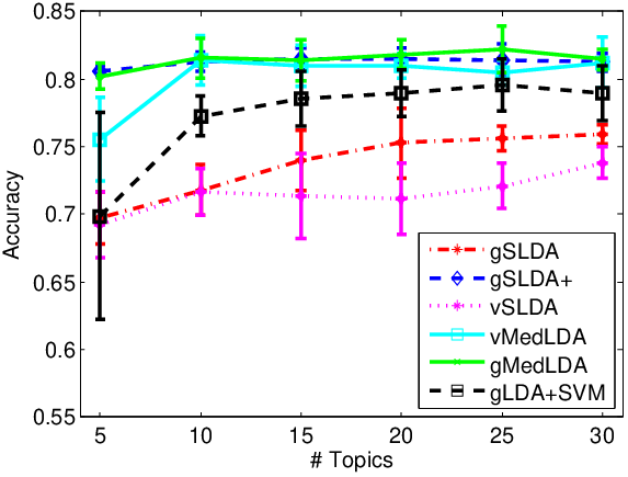
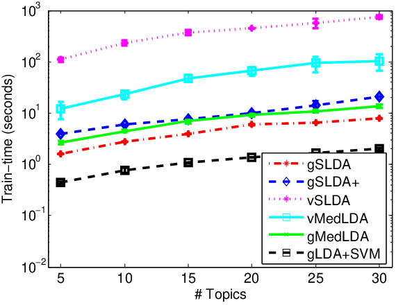
Following the same setting in [\citenameLacoste-Jullien et al.2009, \citenameZhu et al.2012], the task is to distinguish postings of the newsgroup alt.atheism and those of the group talk.religion.misc. The training set contains 856 documents and the test set contains 569 documents. We compare the generalized logistic supervised LDA using Gibbs sampling (denoted by gSLDA) with various competitors, including the standard sLDA using variational mean-field methods (denoted by vSLDA) [\citenameWang et al.2009], the MedLDA model using variational mean-field methods (denoted by vMedLDA) [\citenameZhu et al.2012], and the MedLDA model using collapsed Gibbs sampling algorithms (denoted by gMedLDA) [\citenameJiang et al.2012]. We also include the unsupervised LDA using collapsed Gibbs sampling as a baseline, denoted by gLDA. For gLDA, we learn a binary linear SVM on its topic representations using SVMLight [\citenameJoachims1999]. The results of DiscLDA [\citenameLacoste-Jullien et al.2009] and linear SVM on raw bag-of-words features were reported in [\citenameZhu et al.2012]. For gSLDA, we compare two versions – the standard sLDA with $c=1$ and the sLDA with a well-tuned $c$ value. To distinguish, we denote the latter by gSLDA+. We set $c=25$ for gSLDA+, and set $\alpha=1$ and $M=100$ for both gSLDA and gSLDA+. As we shall see, gSLDA is insensitive to $\alpha$, $c$ and $M$ in a wide range.

Fig. 1 shows the performance of different methods with various numbers of topics. For accuracy, we can draw two conclusions: 1) without making restricting assumptions on the posterior distributions, gSLDA achieves higher accuracy than vSLDA that uses strict variational mean-field approximation; and 2) by using the regularization constant $c$ to improve the influence of supervision information, gSLDA+ achieves much better classification results, in fact comparable with those of MedLDA models since they have the similar mechanism to improve the influence of supervision by tuning a regularization constant. The fact that gLDA+SVM performs better than the standard gSLDA is due to the same reason, since the SVM part of gLDA+SVM can well capture the supervision information to learn a classifier for good prediction, while standard sLDA can’t well-balance the influence of supervision. In contrast, the well-balanced gSLDA+ model successfully outperforms the two-stage approach, gLDA+SVM, by performing topic discovery and prediction jointly⁴⁴ 4 The variational sLDA with a well-tuned $c$ is significantly better than the standard sLDA, but a bit inferior to gSLDA+..

For training time, both gSLDA and gSLDA+ are very efficient, e.g., about 2 orders of magnitudes faster than vSLDA and about 1 order of magnitude faster than vMedLDA. For testing time, gSLDA and gSLDA+ are comparable with gMedLDA and the unsupervised gLDA, but faster than the variational vMedLDA and vSLDA, especially when $K$ is large.

We perform multi-class classification on the 20NG data set with all the 20 categories. For multi-class classification, one possible extension is to use a multinomial logistic regression model for categorical variables $Y$ by using topic representations $\bar{\mathbf{z}}$ as input features. However, it is nontrivial to develop a Gibbs sampling algorithm using the similar data augmentation idea, due to the presence of latent variables and the nonlinearity of the soft-max function. In fact, this is harder than the multinomial Bayesian logistic regression, which can be done via a coordinate strategy [\citenamePolson et al.2012]. Here, we apply the binary gSLDA to do the multi-class classification, following the “one-vs-all” strategy, which has been shown effective [\citenameRifkin and Klautau2004], to provide some preliminary analysis. Namely, we learn 20 binary gSLDA models and aggregate their predictions by taking the most likely ones as the final predictions. We again evaluate two versions of gSLDA – the standard gSLDA with $c=1$ and the improved gSLDA+ with a well-tuned $c$ value. Since gSLDA is also insensitive to $\alpha$ and $c$ for the multi-class task, we set $\alpha=5.6$ for both gSLDA and gSLDA+, and set $c=256$ for gSLDA+. The number of burn-in is set as $M=40$, which is sufficiently large to get stable results, as we shall see.

Fig. 2 shows the accuracy and training time. We can see that: 1) by using Gibbs sampling without restricting assumptions, gSLDA performs better than the variational vSLDA that uses strict mean-field approximation; 2) due to the imbalance between the single supervision and a large set of word counts, gSLDA doesn’t outperform the decoupled approach, gLDA+SVM; and 3) if we increase the value of the regularization constant $c$, supervision information can be better captured to infer predictive topic representations, and gSLDA+ performs much better than gSLDA. In fact, gSLDA+ is even better than the MedLDA that uses mean-field approximation, while is comparable with the MedLDA using collapsed Gibbs sampling. Finally, we should note that the improvement on the accuracy might be due to the different strategies on building the multi-class classifiers. But given the performance gain in the binary task, we believe that the Gibbs sampling algorithm without factorization assumptions is the main factor for the improved performance.

For training time, gSLDA models are about 10 times faster than variational vSLDA. Table 1 shows in detail the percentages of the training time (see the numbers in brackets) spent at each sampling step for gSLDA+. We can see that: 1) sampling the global variables $\boldsymbol{\eta}$ is very efficient, while sampling local variables $(\boldsymbol{\lambda},\mathbf{Z})$ are much more expensive; and 2) sampling $\boldsymbol{\lambda}$ is relatively stable as $K$ increases, while sampling $\mathbf{Z}$ takes more time as $K$ becomes larger. But, the good news is that our Gibbs sampling algorithm can be easily parallelized to speedup the sampling of local variables, following the similar architectures as in LDA.

A Parallel Implementation: GraphLab is a graph-based programming framework for parallel computing [\citenameGonzalez et al.2012]. It provides a high-level abstraction of parallel tasks by expressing data dependencies with a distributed graph. GraphLab implements a GAS (gather, apply, scatter) model, where the data required to compute a vertex (edge) are gathered along its neighboring components, and modification of a vertex (edge) will trigger its adjacent components to recompute their values. Since GAS has been successfully applied to several machine learning algorithms⁵⁵ 5 http://docs.graphlab.org/toolkits.html including Gibbs sampling of LDA, we choose it as a preliminary attempt to parallelize our Gibbs sampling algorithm. A systematical investigation of the parallel computation with various architectures in interesting, but beyond the scope of this paper.

For our task, since there is no coupling among the 20 binary gSLDA classifiers, we can learn them in parallel. This suggests an efficient hybrid multi-core/multi-machine implementation, which can avoid the time consumption of IPC (i.e., inter-process communication). Namely, we run our experiments on a cluster with 20 nodes where each node is equipped with two 6-core CPUs (2.93GHz). Each node is responsible for learning one binary gSLDA classifier with a parallel implementation on its 12-cores. For each binary gSLDA model, we construct a bipartite graph connecting train documents with corresponding terms. The graph works as follows: 1) the edges contain the token counts and topic assignments; 2) the vertices contain individual topic counts and the augmented variables $\boldsymbol{\lambda}$; 3) the global topic counts and $\boldsymbol{\eta}$ are aggregated from the vertices periodically, and the topic assignments and $\boldsymbol{\lambda}$ are sampled asynchronously during the GAS phases. Once started, sampling and signaling will propagate over the graph. One thing to note is that since we cannot directly measure the number of iterations of an asynchronous model, here we estimate it with the total number of topic samplings, which is again aggregated periodically, divided by the number of tokens. We denote the parallel models by parallel-gSLDA ($c=1$) and parallel-gSLDA+ ($c=256$). From Fig. 2 (b), we can see that the parallel gSLDA models are about 2 orders of magnitudes faster than their sequential counterpart models, which is very promising. Also, the prediction performance is not sacrificed as we shall see in Fig. 4.

Burn-In: Fig. 3 shows the performance of gSLDA+ with different burn-in steps for binary classification. When $M=0$ (see the most left points), the models are built on random topic assignments. We can see that the classification performance increases fast and converges to the stable optimum with about 20 burn-in steps. The training time increases about linearly in general when using more burn-in steps. Moreover, the training time increases linearly as $K$ increases. In the previous experiments, we set $M=100$.

Fig. 4 shows the performance of gSLDA+ and its parallel implementation (i.e., parallel-gSLDA+) for the multi-class classification with different burn-in steps. We can see when the number of burn-in steps is larger than 20, the performance of gSLDA+ is quite stable. Again, in the log-log scale, since the slopes of the lines in Fig. 4 (b) are close to the constant 1, the training time grows about linearly as the number of burn-in steps increases. Even when we use 40 or 60 burn-in steps, the training time is still competitive, compared with the variational vSLDA. For parallel-gSLDA+ using GraphLab, the training is consistently about 2 orders of magnitudes faster. Meanwhile, the classification performance is also comparable with that of gSLDA+, when the number of burn-in steps is larger than 40. In the previous experiments, we have set $M=40$ for both gSLDA+ and parallel-gSLDA+.

Regularization constant $c$: Fig. 5 shows the performance of gSLDA in the binary classification task with different $c$ values. We can see that in a wide range, e.g., from 9 to 100, the performance is quite stable for all the three $K$ values. But for the standard sLDA model, i.e., $c=1$, both the training accuracy and test accuracy are low, which indicates that sLDA doesn’t fit the supervision data well. When $c$ becomes larger, the training accuracy gets higher, but it doesn’t seem to over-fit and the generalization performance is stable. In the above experiments, we set $c=25$. For multi-class classification, we have similar observations and set $c=256$ in the previous experiments.

Dirichlet prior $\alpha$: Fig. 6 shows the performance of gSLDA on the binary task with different $\alpha$ values. We report two cases with $c=1$ and $c=9$. We can see that the performance is quite stable in a wide range of $\alpha$ values, e.g., from $0.1$ to $10$. We also noted that the change of $\alpha$ does not affect the training time much.

References

- [Ahmed et al.2012] A. Ahmed, M. Aly, J. Gonzalez, S. Narayanamurthy, and A. Smola. 2012. Scalable inference in latent variable models. In International Conference on Web Search and Data Mining (WSDM).
- [Blei and McAuliffe2010] D.M. Blei and J.D. McAuliffe. 2010. Supervised topic models. arXiv:1003.0783v1.
- [Blei et al.2003] D.M. Blei, A.Y. Ng, and M.I. Jordan. 2003. Latent Dirichlet allocation. JMLR, 3:993–1022.
- [Chen et al.1999] M. Chen, J. Ibrahim, and C. Yiannoutsos. 1999. Prior elicitation, variable selection and Bayesian computation for logistic regression models. Journal of Royal Statistical Society, Ser. B, (61):223–242.
- [Germain et al.2009] P. Germain, A. Lacasse, F. Laviolette, and M. Marchand. 2009. PAC-Bayesian learning of linear classifiers. In International Conference on Machine Learning (ICML), pages 353–360.
- [Globerson et al.2007] A. Globerson, T. Koo, X. Carreras, and M. Collins. 2007. Exponentiated gradient algorithms for log-linear structured prediction. In ICML, pages 305–312.
- [Gonzalez et al.2012] J.E. Gonzalez, Y. Low, H. Gu, D. Bickson, and C. Guestrin. 2012. Powergraph: Distributed graph-parallel computation on natural graphs. In the 10th USENIX Symposium on Operating Systems Design and Implementation (OSDI).
- [Griffiths and Steyvers2004] T.L. Griffiths and M. Steyvers. 2004. Finding scientific topics. Proceedings of National Academy of Science (PNAS), pages 5228–5235.
- [Halpern et al.2012] Y. Halpern, S. Horng, L. Nathanson, N. Shapiro, and D. Sontag. 2012. A comparison of dimensionality reduction techniques for unstructured clinical text. In ICML 2012 Workshop on Clinical Data Analysis.
- [Holmes and Held2006] C. Holmes and L. Held. 2006. Bayesian auxiliary variable models for binary and multinomial regression. Bayesian Analysis, 1(1):145–168.
- [Jiang et al.2012] Q. Jiang, J. Zhu, M. Sun, and E.P. Xing. 2012. Monte Carlo methods for maximum margin supervised topic models. In Advances in Neural Information Processing Systems (NIPS).
- [Joachims1999] T. Joachims. 1999. Making large-scale SVM learning practical. MIT press.
- [Lacoste-Jullien et al.2009] S. Lacoste-Jullien, F. Sha, and M.I. Jordan. 2009. DiscLDA: Discriminative learning for dimensionality reduction and classification. Advances in Neural Information Processing Systems (NIPS), pages 897–904.
- [Lin2001] Y. Lin. 2001. A note on margin-based loss functions in classification. Technical Report No. 1044. University of Wisconsin.
- [McAllester2003] D. McAllester. 2003. PAC-Bayesian stochastic model selection. Machine Learning, 51:5–21.
- [Meyer and Laud2002] M. Meyer and P. Laud. 2002. Predictive variable selection in generalized linear models. Journal of American Statistical Association, 97(459):859–871.
- [Newman et al.2009] D. Newman, A. Asuncion, P. Smyth, and M. Welling. 2009. Distributed algorithms for topic models. Journal of Machine Learning Research (JMLR), (10):1801–1828.
- [Polson et al.2012] N.G. Polson, J.G. Scott, and J. Windle. 2012. Bayesian inference for logistic models using Polya-Gamma latent variables. arXiv:1205.0310v1.
- [Rifkin and Klautau2004] R. Rifkin and A. Klautau. 2004. In defense of one-vs-all classification. Journal of Machine Learning Research (JMLR), (5):101–141.
- [Rosasco et al.2004] L. Rosasco, E. De Vito, A. Caponnetto, M. Piana, and A. Verri. 2004. Are loss functions all the same? Neural Computation, (16):1063–1076.
- [Smola and Narayanamurthy2010] A. Smola and S. Narayanamurthy. 2010. An architecture for parallel topic models. Very Large Data Base (VLDB), 3(1-2):703–710.
- [Tanner and Wong1987] M.A. Tanner and W.-H. Wong. 1987. The calculation of posterior distributions by data augmentation. Journal of the Americal Statistical Association (JASA), 82(398):528–540.
- [van Dyk and Meng2001] D. van Dyk and X. Meng. 2001. The art of data augmentation. Journal of Computational and Graphical Statistics (JCGS), 10(1):1–50.
- [Wang et al.2009] C. Wang, D.M. Blei, and Li F.F. 2009. Simultaneous image classification and annotation. IEEE Conference on Computer Vision and Pattern Recognition (CVPR).
- [Zhu et al.2011] J. Zhu, N. Chen, and E.P. Xing. 2011. Infinite latent SVM for classification and multi-task learning. In Advances in Neural Information Processing Systems (NIPS), pages 1620–1628.
- [Zhu et al.2012] J. Zhu, A. Ahmed, and E.P. Xing. 2012. MedLDA: maximum margin supervised topic models. Journal of Machine Learning Research (JMLR), (13):2237–2278.
- [Zhu et al.2013a] J. Zhu, N. Chen, H. Perkins, and B. Zhang. 2013a. Gibbs max-margin topic models with fast sampling algorithms. In International Conference on Machine Learning (ICML).
- [Zhu et al.2013b] J. Zhu, N. Chen, and E.P. Xing. 2013b. Bayesian inference with posterior regularization and applications to infinite latent svms. arXiv:1210.1766v2.