Interactive Function Computation with Reconstruction Constraints

The problem of computing functions of distributed correlated information sources arises in different networking scenarios, such as sensor networks, cloud computing and smart grids. With limited communication resources, one important goal is to find the most effective way to operate the network in order to exchange minimal information while computing the desired functions with the required accuracy. For scenarios involving sensitive information, in addition to regular distortion constraints at the terminals, each terminal may wish to estimate the function computed at the other terminals within a certain accuracy. This leads to the constrained reconstruction constraint [1]-[2], which as a special case includes common reconstruction constraint [3] where all the terminals are required to agree on the computed function values with probability one.

The classical lossy source coding with side information problem investigated by Wyner and Ziv [4] involves one-way communication from the encoder to the decoder and only considers the distortion incurred in source reconstruction at the decoder. Steinberg [3] considered an additional constraint in which the encoder is also required to reproduce the reconstruction at the decoder exactly, leading to the above common reconstruction constraint. The setting in [3] suggests that while the side information at the decoder can be used to reduce the source rate through the binning process as in the Wyner-Ziv setting, it cannot be further combined with the compression index, thereby resulting in a higher distortion at the decoder. Lapidoth et al [1] extended [3] to allow for some distortion between the encoder’s and the decoder’s reconstruction, leading to the constrained reconstruction constraint.

While the above papers consider information flow from the encoder to the decoder only, Ma and Ishwar studied an interactive communication scenario where the two terminals exchange information in an alternating fashion for lossy function computation [5]. The goal, as in the Wyner-Ziv setting, is to satisfy distortion requirements individually at each terminal. They showed that although for some functions there is no need to use multiple rounds of communication, there are functions for which every additional round of communication, subject to a fixed total sum rate, further decreases distortion.

In this paper we consider two terminal interactive function computation with reconstruction constraints, hence extending the framework in [1] to take into account interaction and in [5] to take into account reconstruction constraints. We assume each terminal computes a different function of the two sources and reconstructs the function computed by the other terminal, all subject to distortion constraints. Multiple rounds of communication are allowed. Communication can take place in a sequential fashion, where terminals take turns, or in a simultaneous fashion. We first identify the general rate-distortion region for this problem. We then study the Gaussian case with common reconstruction and compare sequential and simultaneous rate-distortion regions for different functions. Overall, our results highlight the importance of interaction under reconstruction constraints.

It is known that the coordination problem of [6] is closely related to rate-distortion with side information. In particular, interactive coordination framework of [7] can be used to study the problem investigated in this paper. Apart from giving an explicit characterization for the rate-distortion region with reconstruction constraints, we identify the individual set of rates for each communication round, while [7] only considers sum rates.

We consider a two-terminal interactive function computation problem with $t$ rounds of communication as shown in Fig 1. Here the “round” refers to a one-way communication session between two terminals. Terminal A, $\mathbb{T}_{A}$, observes source $X^{n}$, and terminal B, $\mathbb{T}_{B}$, observes $Y^{n}$. The sources are drawn i.i.d $\sim p(x,y)$. The objective of $\mathbb{T}_{k}$ is to compute the function $Z_{k}^{n}={f}_{k}^{(n)}(X^{n},Y^{n})=(f_{k}(X_{1},Y_{1}),\ldots,f_{k}(X_{n},Y_{n})),k=A,B$ in a lossy fashion and with reconstruction constraints [1]. Corresponding distortion measures and constraints will be discussed below.

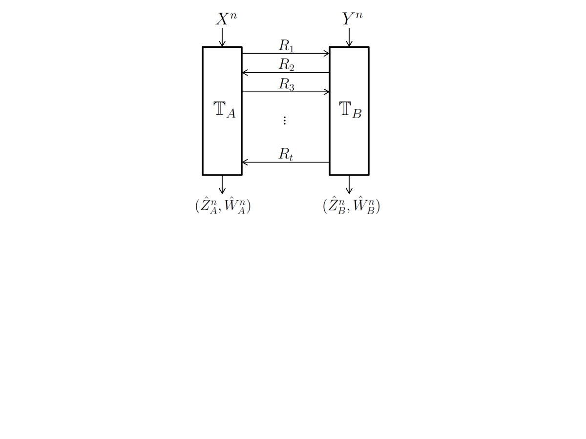
The messages sent in $t$ rounds of communication are denoted as $M_{1},\dots,M_{t}$. These messages are sent sequentially starting from $\mathbb{T}_{A}$ (or $\mathbb{T}_{B}$). Alternatively, assuming $t$ is even, the terminals can send their messages simultaneously, with the pair $(M_{j},M_{j+1}),j=2k-1,k=1,2,\dots,t/2$ transmitted at the same time. Below, we define encoding and decoding functions for sequential transmission starting from $\mathbb{T}_{A}$; definitions for sequential transmission starting from $\mathbb{T}_{B}$ or for simultaneous transmission similarly follow.

A message sent from $\mathbb{T}_{A}$ can depend on $X^{n}$ and all previously communicated messages. In a similar manner each message sent from $\mathbb{T}_{B}$ can depend on $Y^{n}$ and all previous messages. More formally, we can define encoding functions as follows:

	$\displaystyle M_{j}=\phi^{(n)}_{j}$	$\displaystyle(X^{n},M^{j-1})$	$\displaystyle\hbox{ ,}\verb" "j\hbox{ odd;}$
	$\displaystyle M_{j}=\phi^{(n)}_{j}$	$\displaystyle(Y^{n},M^{j-1})$	$\displaystyle\hbox{ ,}\verb" "j\hbox{ even;}$

where

	$\displaystyle\phi^{(n)}_{j}$	$\displaystyle:\mathcal{X}^{n}\times\prod_{k=1}^{j-1}\mathcal{M}_{k}\mapsto\mathcal{M}_{j}$	$\displaystyle\hbox{ ,}\verb" "j\hbox{ odd;}$
	$\displaystyle\phi^{(n)}_{j}$	$\displaystyle:\mathcal{Y}^{n}\times\prod_{k=1}^{j-1}\mathcal{M}_{k}\mapsto\mathcal{M}_{j}$	$\displaystyle\hbox{ ,}\verb" "j\hbox{ even.}$

and $\mathcal{M}_{j}=\{1,2,\dots,2^{nR_{j}}\}$ where $R_{j}$ is the rate of the $j$’th message. We assume $M_{0}=1$ is deterministic. Note that $\phi_{j}$ corresponds to the encoding operations at $\mathbb{T}_{A}$, for $j$ odd, and encoding operations at $\mathbb{T}_{B}$, for $j$ even. After $t$ rounds of communication, each terminal computes its desired function using $\Psi_{k},k=A,B$ as follows:

	$\displaystyle\hat{Z}_{A}^{n}=\Psi_{A}^{(n)}(X^{n},M^{t})$		(1)
	$\displaystyle\hat{Z}_{B}^{n}=\Psi_{B}^{(n)}(Y^{n},M^{t})$		(2)

Furthermore, each terminal also computes an estimate of the other terminal’s function using $\psi_{k},k=A,B$, as follows

	$\displaystyle\hat{W}_{A}^{n}=\psi_{A}^{(n)}(X^{n},M^{t})$		(3)
	$\displaystyle\hat{W}_{B}^{n}=\psi_{B}^{(n)}(Y^{n},M^{t})$		(4)

The tuple $(\phi_{1}^{(n)},\dots,\phi_{t}^{(n)},\Psi_{A}^{(n)},\Psi_{B}^{(n)},\psi_{B}^{(n)},\psi_{A}^{(n)})$ is called an $(n,R_{1},\dots,R_{t},D_{A},D_{B},D_{AB},D_{BA})$-code if the produced sequences $\hat{Z}_{A}^{n}$, $\hat{Z}_{B}^{n}$, $\hat{W}_{A}^{n}$ and $\hat{W}_{B}^{n}$ satisfy

	$\displaystyle\frac{1}{n}\sum_{i=1}^{n}Ed_{A}(Z_{A}{}_{,i},\hat{Z}_{A}{}_{,i})\leq D_{A}$		(5)
	$\displaystyle\frac{1}{n}\sum_{i=1}^{n}Ed_{AB}(\hat{Z}_{A}{}_{,i},\hat{W}_{B}{}_{,i})\leq D_{AB}$		(6)
	$\displaystyle\frac{1}{n}\sum_{i=1}^{n}Ed_{B}(Z_{B}{}_{,i},\hat{Z}_{B}{}_{,i})\leq D_{B}$		(7)
	$\displaystyle\frac{1}{n}\sum_{i=1}^{n}Ed_{BA}(\hat{Z}_{B}{}_{,i},\hat{W}_{A}{}_{,i})\leq D_{BA}$		(8)

where $d_{k}(.,.)$ and $d_{kl}(.,.)$, $k,l=A,B$, $k\not=l,$ are single letter distortion measures and $Z_{k}{}_{,i}={f}_{k}(X_{i},Y_{i})$ is the actual value of the desired function at $\mathbb{T}_{k}$, $k=A,B$. Note that (5) and (7) are the usual distortion constraints for computing ${f}_{k}(X,Y)$ at $\mathbb{T}_{k}$, $k=A,B$, whereas constraints (6) and (8) are the constrained reconstruction constraints [1]. The rate and distortion tuple $(R_{1},\dots,R_{t},D_{A},D_{B},D_{AB},D_{BA})$ is achievable if for any $\epsilon\geq 0$ and $n$ sufficiently large there exist an $(n,R_{1}+\epsilon,\dots,R_{t}+\epsilon,D_{A}+\epsilon,D_{B}+\epsilon,D_{AB}+\epsilon,D_{BA}+\epsilon)$-code. The set of all achievable $(R_{1},\dots,R_{t},D_{A},D_{B},D_{AB},D_{BA})$ is denoted by $\mathfrak{R}^{(t)}$ and the constrained-reconstruction rate-distortion region for $t$-round interactive communication is given by:

	$\displaystyle\mathcal{R}^{(t)}(D_{A},D_{B},D_{AB},D_{BA})\triangleq$
	$\displaystyle\bigg\{(R_{1},\dots,R_{t})|(R_{1},\dots,R_{t},D_{A},D_{B},D_{AB},D_{BA})\in\mathfrak{R}^{(t)}\bigg\}$

Similarly, we can define common-reconstruction rate-distortion region $\mathcal{R}^{(t)}_{CR}(D_{A},D_{B})$ by replacing conditions (6) and (8) with

	$\displaystyle Pr(\hat{W}_{B}^{n}\neq\hat{Z}_{A}^{n})\leq\epsilon_{n}$		(9)
	$\displaystyle Pr(\hat{W}_{A}^{n}\neq\hat{Z}_{B}^{n})\leq\epsilon_{n}$		(10)

where $\epsilon_{n}$ goes to zero as $n\rightarrow\infty$.

In this section, we provide a characterization of the rate-distortion region for $t$-round interactive function computation with reconstruction constraints for general discrete memoryless sources. Hence we assume the alphabet sets $\mathcal{X},\mathcal{Y},\hat{\mathcal{Z}}_{A},\hat{\mathcal{Z}}_{B},\hat{\mathcal{W}}_{A}$ and $\hat{\mathcal{W}}_{B}$ are all discrete.

In this section, we illustrate the common reconstruction rate-distortion region, $\mathcal{R}^{(t)}_{CR}(D_{A},D_{B})$, for jointly Gaussian sources. We set $d(a,b)=(a-b)^{2}$ for the distortion functions in (5) and (7). We first consider linear functions of $X$ and $Y$. We then study extensions to other functions.

In this paper we have studied the interactive function computation with reconstruction constraints and characterized the constrained and common reconstruction rate-distortion regions. We have also evaluated the common-reconstruction rate-distortion region for linear functions of Gaussian sources. An interesting observation we have made is that two simultaneous rounds of communication are optimal in this case. A comparison with one-way communication has shown that a significant performance improvement is possible when interaction is allowed.

References

- [1] A. Lapidoth, A. Malär, and M. Wigger, “Constrained Wyner-Ziv coding,” in IEEE ISIT, August 2011, pp. 1076 –1080.
- [2] A. Lapidoth, A. Malär, and M. A. Wigger, “Constrained source coding with side information,” available at http://arxiv.org/abs/1301.5109, 2013.
- [3] Y. Steinberg, “Coding and common reconstruction,” IEEE Trans. on Info. Theory, vol. 55, no. 11, pp. 4995–5010, 2009.
- [4] A. Wyner and J. Ziv, “The rate-distortion function for source coding with side information at the decoder,” IEEE Trans. on Info. Theory, vol. 22, no. 1, pp. 1 – 10, Janaury 1976.
- [5] N. Ma and P. Ishwar, “Some results on distributed source coding for interactive function computation,” IEEE Trans. on Info. Theory, vol. 57, no. 9, pp. 6180 –6195, September 2011.
- [6] P. Cuff, “Communication in networks for coordinating behavior,” Ph.D. dissertation, Dep. of ECE of Stanford University, July 2009.
- [7] M. Yassaee, A. Gohari, and M. Aref, “Channel simulation via interactive communications,” in IEEE ISIT, July 2012, pp. 3053 –3057.
- [8] W. Gu, “On achievable rate regions for source coding over networks,” Ph.D. dissertation, California Institute of Technology, August 2009.
- [9] S. Jalali and M. Effros, “Separation of source-network coding and channel coding in wireline networks,” available at http://arxiv.org/abs/1110.3559, 2011.
- [10] A. El Gamal and Y.-H. Kim, Network Information Theory. Cambridge University Press, 2011.