Automatic code generator for higher order integrators

Journal: journal

Asif Mushtaq Email: Asif.Mushtaq@math.ntnu.no Address: Institutt for matematiske fag, NTNU, N-7491 TRONDHEIM, Norway Kåre Olaussen Email: Kare.Olaussen@ntnu.no Address: Institutt for fysikk, NTNU, N-7491 TRONDHEIM, Norway

Abstract

Some explicit algorithms for higher order symplectic integration of a large class of Hamilton’s equations have recently been discussed by Mushtaq et. al. Here we present a Python program for automatic numerical implementation of these algorithms for a given Hamiltonian, both for double precision and multiprecision computations. We provide examples of how to use this program, and illustrate behaviour of both the code generator and the generated solver module(s).

Keywords:

Splitting methods , Modified integrators , Higher order methods , Automatic code generation

2010 MSC

33F05 , 37M15 , 46N40 , 65P10 , 74S30

PROGRAM SUMMARY

Manuscript Title: Automatic code generator for higher order integrators.
Authors: Asif Mushtaq, Kåre Olaussen.
Program Title: HOMsPy: Higher Order (Symplectic) Methods in Python
Journal Reference:
Catalogue identifier:
Licensing provisions: None.
Programming language: Python 2.7.
Computer: PC’s or higher performance computers.
Operating system: Linux, MacOS, MSWindows.
RAM: Kilobytes to a several gigabytes (problem dependent).
Number of processors used: 1
Keywords: Splitting methods, Modified integrators, Higher order methods, Automatic code generation.
Classification: 4.3 Differential equations, 5 Computer Algebra.
External routines/libraries: SymPy library [1] for generating the code. NumPy library [2], and optionally mpmath [3] library for running the generated code. The matplotlib [4] library for plotting results.
Nature of problem: We have developed algorithms [5] for numerical solution of Hamilton’s equations,

\displaystyle\dot{q}^{a}=\frac{\partial H(\bm{q},\bm{p})}{\partial p_{a}},\hskip 9.24994pt\dot{p}_{a}=-\frac{\partial H(\bm{q},\bm{p})}{\partial q^{a}},\hskip 9.24994pta=1,\ldots,\mathcal{N}

(1)

for Hamiltonians of the form

H(\bm{q},\bm{p})=T(\bm{p})+V(\bm{q})=\frac{1}{2}\bm{p}^{T}M\bm{p}+V(\bm{q}),

(2)

with $M$ a symmetric positive definite matrix. The algorithms preserve the symplectic property of the time evolution exactly, and are of orders $\tau^{N}$ (for $2\leq N\leq 8$ ) in the timestep $\tau$ . Although explicit, the algorithms are time-consuming and error-prone to implement numerically by hand, in particular for larger $N$ .
Solution method: We use computer algebra to perform all analytic calculations required for a specific model, and to generate the Python code for numerical solution of this model, including example programs using that code.
Restrictions: In our implementation the mass matrix is assumed to be equal to the unit matrix, and $V(\bm{q})$ must be sufficiently differentiable.
Running time: Subseconds to eons (problem dependent). See discussion in the main article. Program: Python program can be provided on demand from authors.

References

[1] SymPy Developement Team, http://sympy.org/
[2] NumPy Developers, http://numpy.org/
[3] Fredrik Johansson et. al., Python library for arbitrary–precision floating-point arithmetic, http://code.google.code/p/mpmath/ (2010)
[4] J.D. Hunter, Matplotlib: A 2D graphics environment, Computing in Science & Engineering 9, 90–95 (2007)
[5] A. Mushtaq, A. Kværnø, K. Olaussen, Higher order Geometric Integrators for a class of Hamiltonian systems, International Journal of Geometric Methods in Modern Physics, vol 11, no. 1 (2014), 1450009-1–1450009-20. DOI: 10.1142/S0219887814500091. arXiv.org:1301.7736

1 Introduction

The Hamilton equations of motion (1) play an important role in physics and mathematics. They often require numerical methods for solution [1, 2, 3]. A well-behaved class of such methods are the symplectic solvers, which preserve symplecticity of the time evolution exactly. One simple way to construct a symplectic solver is to split the time evolutions into kicks,

\displaystyle\dot{q}^{a}=0,\quad\dot{p}_{a}=-\frac{\partial V(\bm{q})}{\partial q^{a}},

(3)

which is straightforward to integrate to give

	$\displaystyle q^{a}(t+\tau)$	$\displaystyle=q^{a}(t),$		(4)
	$\displaystyle p_{a}(t+\tau)$	$\displaystyle=p_{a}(t)-\tau\frac{\partial V(\bm{q}(t),\bm{p}(t))}{\partial q^{a}},$		(5)

followed by moves,

\displaystyle\dot{q}^{a}=\frac{\partial T(\bm{p})}{\partial p_{a}}=\sum_{b}M^{ab}p_{b},\quad\dot{p}_{a}=0,

(6)

which integrates to

	$\displaystyle q^{a}(t+\tau)$	$\displaystyle=q^{a}(t)+\tau\sum_{b}M^{ab}p_{b}(t+\tau),$
	$\displaystyle p_{a}(t+\tau)$	$\displaystyle=p_{a}(t)-\tau\frac{\partial V(\bm{q}(t),\bm{p}(t))}{\partial q^{a}}.$

This scheme was already introduced by Newton [4] (as more accessible explained by Feynman [5]). A symmetric scheme is to make a kick of size $\frac{1}{2}\tau$ , a move of size $\tau$ , and a kick of size $\frac{1}{2}\tau$ (and repeating). This is often referred to as the Störmer-Verlet method [6, 7]; it has a local error of order $\tau^{3}$ . The solution provided by this method can be viewed as the exact solution of a slightly different Hamiltonian system, with a Hamiltonian $H_{\text{SV}}$ which differ from (2) by an amount proportional to $\tau^{2}$ . For this reason the scheme respects long-time conservation of energy to order $\tau^{2}$ . It will also exactly preserve conservation laws due to Nöther symmetries which are common to $T(\bm{p})=\frac{1}{2}\bm{p}^{T}\bm{M}\bm{p}$ and $V(\bm{q})$ , like momentum and angular momentum which are often preserved in physical models [8].

Recently Mushtaq et. al. [9, 10] proposed some higher order extensions of the Störmer-Verlet scheme. These extensions are also based on the kick-move-kick idea, only with modified Hamiltonians,


$\displaystyle H_{1}$	$\displaystyle\equiv T_{\text{eff}}=\frac{1}{2}\bm{p}^{T}M\bm{p}+\sum_{k\geq 1}T_{2k}(\bm{q},\bm{p}),$	(7a)
$\displaystyle H_{2}$	$\displaystyle\equiv V_{\text{eff}}=V(\bm{q})+\sum_{k\geq 1}V_{2k}(\bm{q}),$	(7b)

where $T_{2k}$ and $V_{2k}$ are proportional to $\tau^{2k}$ . I.e., the proposal is to replace $V(\bm{q})$ in equation (3) by $V_{\text{eff}}(\bm{q})$ , and $T(\bm{p})$ in equation (6) by $T_{\text{eff}}(\bm{q},\bm{p})$ . The goal is to construct $V_{\text{eff}}$ and $T_{\text{eff}}$ such that the combined kick-move-kick process corresponds to an evolution by a Hamiltonian $H_{\text{eff}}$ which lies closer to the Hamiltonian $H$ of equation (2). The difference being of order $\tau^{2N+2}$ when summing terms to $k=N$ in equations (7).

One problem with this approach is that $T_{\text{eff}}$ in general will depend on both $\bm{q}$ and $\bm{p}$ ; hence the move-steps of equation (6) can no longer be integrated explicitly. To overcome this problem we introduce a generating function [3]

{G}(\bm{q},\bm{P};\tau)=\sum_{0\leq k\leq N}{G}_{k}(\bm{q},\bm{P})\,\tau^{k}

(8)

such that the transformation $\left(\bm{q},\bm{p}\right)\rightarrow\left(\bm{Q},\bm{P}\right)$ defined by


$\displaystyle p_{a}$	$\displaystyle=\frac{\partial{G}}{\partial q^{a}},$	(9a)
$\displaystyle Q^{a}$	$\displaystyle=\frac{\partial{G}}{\partial P_{a}},$	(9b)

preserves the symplectic structure exactly, and reproduce the time evolution generated by $T_{\text{eff}}$ to order $\tau^{N}$ . Here $Q^{a}$ is shorthand for $q^{a}(t+\tau)$ , and $P_{a}$ shorthand for $p_{a}(t+\tau)$ . Equation (9a) is implicit and in general nonlinear, but the nonlinearity is of order $\tau^{3}$ (hence small for practical values of $\tau$ ). In the numerical code we solve (9a) by straightforward iteration (typically two to four iterations in the cases we have investigated).

The rest of this paper is organized as follows: In section 2 we introduce compact notation in which we present the general explicit expressions for $T_{\text{eff}}(\bm{q},\bm{p})$ , $V_{\text{eff}}(\bm{q})$ , and $G(\bm{q},\bm{Q})$ . Because of their compactness these expressions are straightforward to implement in SymPy.

In section 3 we provide examples of how to use the code generator on specific problems. This process proceeds through two stages: (i) By providing the potential $V(\bm{q})$ (possibly depending on extra parameters) code for solving the resulting Hamilton’s equations (the solver module) is generated, and (ii) this solver module is used to analyse the model. The last stage must of course be implemented by the user, but an example program which explicitly demonstrates how the solver module can be used is also generated during the first stage.

The examples given in subsections 3.1 (Vibrating beam) and 3.2 (One-parameter family of quartic anharmonic oscillators) have known exact solutions; this makes it easy to check whether the algorithms behave like expected with respect to accuracy. The example in subsection 3.3 (two-dimensional pendulum) demonstrates that the program can handle nonpolynomial functions, and that it generates code which preserves angular momentum exactly.

In section 4 we consider a collection of many coupled quartic oscillators. This is intended as a stress-test of the code, investigating how it behaves with respect to precision as well as time and memory use for larger and more complex models. Test of both of the code-generating process, and of the solver modules generated. We find that the latter continue to behave as expected with respect to accuracy, but that there is room for improvement in the area of time and memory efficiency, in particular for large structured systems.

In section 5 we present the organization of our code generating program itself, including diagrammatic representations of its structure. We finally summarize our experiences in section 6.

2 Explicit expressions

Compact explicit expressions for the terms of order $\tau^{N}$ for $N\in\left\{2,4,6\right\}$ in equations (7) were given in [9, 10]. With the notation

\displaystyle\partial_{a}\equiv\frac{\partial}{\partial q^{a}},\quad\partial^{a}\equiv M^{ab}\partial_{b},\quad p^{a}\equiv M^{ab}p_{b},\quad D\equiv p_{a}\partial^{a},\quad\bar{D}\equiv(\partial_{a}V)\partial^{a},

(10)

where the Einstein summation convention¹¹ 1 An index which occur twice, once in lower position and once in upper position, are implicitly summed over all available values. I.e, $M^{ab}\partial_{b}\equiv\sum_{b}M^{ab}\partial_{b}$ (we generally use the matrix $M$ to rise an index from lower to upper position). is employed, they are


$\displaystyle T_{2}$	$\displaystyle=-\frac{1}{12}D^{2}V\tau^{2},$	(11a)
$\displaystyle T_{4}$	$\displaystyle=\frac{1}{720}\left(D^{4}-9\bar{D}D^{2}+3D\bar{D}\right)V\tau^{4},$	(11b)
$\displaystyle T_{6}$	$\displaystyle=-\frac{1}{60480}\big(2\,D^{6}-40\,\bar{D}D^{4}+46\,D\bar{D}D^{3}-15\,D^{2}\bar{D}D^{2}$
	$\displaystyle+54\,\bar{D}^{2}D^{2}-9\,\bar{D}D\bar{D}D-42\,D\bar{D}^{2}D+12\,D^{2}\bar{D}^{2}\big)V\tau^{6}$	(11c)
$\displaystyle V_{2}$	$\displaystyle=\frac{1}{24}\bar{D}V\tau^{2},$	(11d)
$\displaystyle V_{4}$	$\displaystyle=\frac{1}{480}\bar{D}^{2}V\tau^{4},$	(11e)
$\displaystyle V_{6}$	$\displaystyle=\frac{1}{161280}\left(17\,\bar{D}^{3}-10\,\bar{D}_{3}\right)V\tau^{6}.$	(11f)

In the last line we have introduced

\bar{D}_{3}\equiv(\partial_{a}V)(\partial_{b}V)(\partial_{c}V)\partial^{a}\partial^{b}\partial^{c}.

(12)

By introducing the operator $\mathcal{D}=P^{a}\partial_{a}$ the explicit expressions for the coefficients ${G}_{k}$ can be written


$\displaystyle{G}_{0}$	$\displaystyle=q^{a}P_{a},$	(13a)
$\displaystyle{G}_{1}$	$\displaystyle={\textstyle\frac{1}{2}}P^{a}P_{a},$	(13b)
$\displaystyle{G}_{2}$	$\displaystyle=0,$	(13c)
$\displaystyle{G}_{3}$	$\displaystyle=-{\textstyle\frac{1}{12}}{\cal D}^{2}V,$	(13d)
$\displaystyle{G}_{4}$	$\displaystyle=-{\textstyle\frac{1}{24}}{\cal D}^{3}V,$	(13e)
$\displaystyle{G}_{5}$	$\displaystyle=-{\textstyle\frac{1}{240}}\left(3\,{\cal D}^{4}+3\,\bar{D}{\cal D}^{2}-{\cal D}\bar{D}{\cal D}\right)V,$	(13f)
$\displaystyle{G}_{6}$	$\displaystyle=-{\textstyle\frac{1}{720}}\left({2\,\cal D}^{5}+8\,\bar{D}{\cal D}^{3}-5\,{\cal D}\bar{D}{\cal D}^{2}\right)V,$	(13g)
$\displaystyle{G}_{7}$	$\displaystyle=-{\textstyle\frac{1}{20160}}\Big({10\,\cal D}^{6}+10\,\bar{D}{\cal D}^{4}+90\,{\cal D}\bar{D}{\cal D}^{3}-75\,{\cal D}^{2}\bar{D}{\cal D}^{2}$
	$\displaystyle\phantom{=-{\textstyle\frac{1}{20160}}}\,+\,18\,\bar{D}^{2}{\cal D}^{2}-3\,\bar{D}{\cal D}\bar{D}{\cal D}-14\,{\cal D}\bar{D}^{2}{\cal D}+4\,{\cal D}^{2}\bar{D}^{2}\Big)V,$	(13h)
$\displaystyle{G}_{8}$	$\displaystyle=-{\textstyle\frac{1}{40320}}\Big(3\,{\cal D}^{7}-87\,\bar{D}{\cal D}^{5}+231\,{\cal D}\bar{D}{\cal D}^{4}-133\,{\cal D}^{2}\bar{D}{\cal D}^{3}+63\,\bar{D}^{2}{\cal D}^{3}$
	$\displaystyle\phantom{=-{\textstyle\frac{1}{40320}}}\,-3\,{\cal D}\bar{D}^{2}{\cal D}^{2}-21\,{\cal D}^{2}\bar{D}^{2}{\cal D}+\,4\,{\cal D}^{3}\bar{D}^{2}-63\,\bar{D}{\cal D}\bar{D}{\cal D}^{2}$	(13i)
	$\displaystyle\phantom{=-{\textstyle\frac{1}{40320}}}+25\,{\cal D}\bar{D}{\cal D}\bar{D}{\cal D}\Big)V.$

The equations (11,13), when used in equations (3,9), define the kick-move-kick scheme for a general potential $V$ . If one uses all the listed terms the local error becomes of order $\tau^{9}$ , and the scheme will respect long-time conservation of energy to order $\tau^{8}$ .

However, explicit implementation of the numerical code for a specific potential is rather laborious and error-prone to do by hand, since the repeated differentiations (with respect to many variables) and multiplications by lengthy expressions are usually involved. We have therefore written a code-generating program in SymPy, wich takes a given potential $V$ as input, perform all the necessary algebra symbolically, and automatically constructs a Python module for solving one full kick-move-kick timestep. It also writes a Python program example using the module; this example may serve as a template for larger applications.

3 Examples of code generation

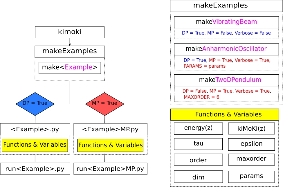
The submitted code includes a file makeExamples.py, with various examples which demonstrate how the code generator can be used. We go through these examples in this section; they also provide some illustrations of how the integrators perform in practical use.

3.1 Vibrating beam

A simple model for a vibrating beam is defined by the Hamiltonian

H=\frac{1}{2}p^{2}-\frac{1}{2}q^{2}+\frac{1}{4}q^{4}.

(14)

A Python code snippet which generates a numerical solver for this problem is the following:

⬇

1 def makeVibratingBeam():

2 #Choose names for coordinate and momentum

3 q, p = sympy.symbols([’q’, ’p’])

4 qvars = [q]; pvars = [p]

5 #Define the potential in terms of the coordinate

6 V = -q*q/2 + q**4/4

7 #Create code for a double-precision solver

8 kimoki.makeModules(’VibratingBeam’, V, qvars, pvars)

Creating a module for solving a vibrating beam

Line 8 generates the files VibratingBeam.py and runVibratingBeam.py. The file VibratingBeam.py contains the general double precision solver module for this problem. A simple use of it in an interactive session is illustrated below:

⬇

1 >>> from __future__ import division

2 >>> from VibratingBeam import *

3 >>> z = numpy.array([1/2, 5/4])

4 >>> kiMoKi(z); print z

5 [ 0.62690658 1.28822851]

6 >>> kiMoKi(z); print z

7 [ 0.75756578 1.32399846]

Interactive use of the solver module

Here z = [q, p] is a NumPy array containing the current state of the solution. Each call of kiMoKi updates this state (data from previous timesteps are not kept).

The file runVibratingBeam.py is a small example program demonstrating basic use of VibratingBeam.py. A code snippet illustrating some essential steps is:

⬇

1 #Select your preferred number of timesteps, order and timestep

2 nMax = 161

3 VibratingBeam.order = 8; VibratingBeam.tau = 1/10

4 z = numpy.array([1/2, 5/4]) #Initial condition

5 for n in xrange(nMax):

6 VibratingBeam.kiMoKi(z) #Integrate one full timestep

Time evolution of a vibrating beam

The equation is integrated in line 6. The complete code in runVibratingBeam.py is an extension of this snippet. The initial condition is generated at random, and saved for possible reuse. Also the complete solution is saved to a (temporary) file for further processing, together with the parameters tau, order, and nMax. By running the file runVibratingBeam.py a single solution is first generated and afterwards displayed in a plot. The plot is also saved in the file VibratingBeam_Soln.png. This plot will look similar to Figure 1.

Figure 1: Example solution of a vibrating beam with random initial conditions. Here

z_{0}

denotes the position

q

, and

z_{1}

the momentum

p

To give some impression of the quality of the generated solution, and how this depends on the timestep and order of the integrator, the example runfile also make a set of runs with the same initial condition, but various values of tau, order, and nMax. A simple quality measure, which is straightforward to implement in general, is how well the initial energy is preserved as time increases. This quantity is plotted, with the plot first displayed and next saved in the file VibratingBeam_EgyErr.png. The plot will look similar to Figure 2. If one prefers to save the plots as .pdf-files the code
#import mathplotlib; matplotlib.use(’PDF’) # Uncomment to ...
on line 17 of the example runfile must be uncommented (then the plot will most likely not be displayed on screen). During the run process solution data is saved to several .pkl-files; these are normally removed after the data has been plotted. To keep this data the code
os.remove(filename) #Comment out to keep datafile
on lines 108 and/or 202 of the example runfile must be commented out.

Figure 2: Example of how well energy is conserved for integrators of various orders

N

, and how the energy errors scale as expected with the timestep

\tau

. The error decreases like

\tau^{N}

when

\tau

decreases. In this case, with a periodic solution, there is also a periodic variation in the energy error.

As illustrated by Figure 2, and verified by all other cases we have investigated, the energy error scales like $\tau^{N}$ , where $\tau$ is the timestep and $N$ is the order of the integrator. The energy error does not grow with time, but varies in a periodic manner — following the periodicity of the generated solution. Note that the integration module, in this case VibratingBeam, contains a parameter epsilon which governs how accurate (9a) is solved. We have observed a systematic growth in the energy error when this parameter is chosen too large, thereby violating symplecticity (too much).

Another property of interest and importance is how the average time per integration step varies with the order of the method. The run example prints a measure of the computer time used. The results of this, for a longer run than the unmodified run example, are shown in Table 1. As can be seen, the penalty of using a higher order method is quite modest for a simple model like the vibrating beam, in particular when the timestep $\tau$ is small.

$N$	$\tau=0.2$	$\tau=0.1$	$\tau=0.05$
2	0.26	0.26	0.26
4	1.03	0.84	0.73
6	1.23	1.01	0.88
8	1.54	1.25	1.09

Table 1: Evaluation time per integration step in milliseconds, dependent on timestep

\tau

and method order

N

. The higher order methods (

N>2

) run faster for smaller

\tau

because the iterative solution of (9a) requires fewer iterations, hence becomes faster. This example, like all others, have been run on a workstation equipped with two four-core Intel Xeon E5520 processors. The ratio between numbers like those above are probably more relevant that their absolute values.

Figure 3: Comparison of the exact elliptic solution (16) with those found by our automatically generated numerical code, for the initial condition

q_{0}=\sqrt{2}+10^{-6}

and

p_{0}=0

, with timestep

\tau=10^{-1}

. The thick blue [red] lines show the numerical solutions for

q(t)

[

p(t)

], the thin blue [red] lines show the exact solution for

q(t)

[

p(t)

The exact solution of this problem can be expressed in terms of Jacobi elliptic functions, cf. equations (16) below. This allows direct comparison between the exact and the numerical solutions, as shown in Figure 3. The initial condition is chosen such that the energy is close to the critical energy, $E=0$ , where the solutions bifurcates from motion over the potential hill at $q=0$ to motion in only one of the two potential wells. The exact solution moves over the potential hill. As can be seen, this is respected by the solutions of order $N=6$ and $8$ , but not by the solutions of order $N=2$ (Störmer-Verlet) and $4$ . This demonstrates that there may be cases where a higher order method, or an impractically small stepsize $\tau$ , is required to obtain even the qualitatively correct solution.

Up to the time $t$ we have computed and plotted the solutions, the order $N=8$ numerical solution cannot be visually distinguished from the exact one in this plot. A difference would become visible for sufficiently large $t$ , because the two solutions have slighly different periods. The difference in periods is of order $\tau^{8}$ for $N=8$ .

3.2 One-parameter family of quartic anharmonic oscillators

A generalization of the previous problem is the class of non-linear oscillators defined by the Hamiltonian

H=\frac{1}{2}p^{2}+\frac{1}{2}\alpha\,q^{2}+\frac{1}{4}q^{4}.

(15)

A one-parameter class of exact solutions to this problem can be expressed in terms of Jacobi elliptic functions [11],


$\displaystyle q(t)$	$\displaystyle=q_{0}\,\text{cn}(\nu t\|\text{k}),$	(16a)
$\displaystyle p(t)$	$\displaystyle=-q_{0}\nu\,\text{sn}(\nu t\|\text{k})\,\text{dn}(\nu t\|\text{k}).$	(16b)

Here the initial conditions are $q(0)=q_{0}$ , and $p(0)=0$ . The vibrating beam discussed in the previous subsection corresponds to the case of $\alpha=-1$ . Equations (16) exhaust the set of solutions which have a maximum at $q_{0}>0$ (or a minimum at $q_{0}<0$ ). This condition imposes the restriction that $\alpha+q^{2}_{0}\geq 0$ . The parameters and energy of the solution are

\nu=\left(\alpha+q^{2}_{0}\right)^{1/2},\qquad k=2^{-1/2}\,q_{0}/\nu,\qquad E=\frac{1}{2}\alpha\,q_{0}^{2}+\frac{1}{4}q_{0}^{4}.

(17)

For $\alpha+\frac{1}{2}q^{2}_{0}>0$ the energy is positive, and $q(t)$ oscillates symmetrically around $q=0$ ; for $\alpha+\frac{1}{2}q^{2}_{0}<0$ the energy is negative, and $q(t)$ oscillates in one of the two possible potential wells (depending on the sign of $q_{0}$ ). For $\alpha+q^{2}_{0}<0$ the solution has a minimum at $q_{0}>0$ (or maximum at $q_{0}<0$ ).²² 2 In which case the solution can be written $q(t)=q_{0}\,\text{nd}(\nu t,k),\qquad p(t)=\nu q_{0}\,k^{2}\,\text{sd}(\nu t,k)\,\text{cd}(\nu t,k),$ (18) with $\nu=\left(-\alpha-q^{2}_{0}/2\right)^{1/2}$ and $k=\nu^{-1}\left(-\alpha-q_{0}^{2}\right)^{1/2}$ . In (16) the modulus $k>1$ when $\alpha+q_{0}^{2}/2<0$ . An alternative expression, with $0<k<1$ , is $q(t)=q_{0}\,\text{dn}(\nu t,k),\qquad p(t)=-\nu q_{0}\,\text{sn}(\nu t,k)\,\text{cn}(\nu t,k),$ (19) where $\nu=2^{-1/2}q_{0}$ and $k=q_{0}^{-1}\left[2(\alpha+q^{2}_{0})\right]^{1/2}$ .

A code snippet for generating numerical solvers for this problem is the following

⬇

1 def makeAnharmonicOscillator():

2 #Choose names for coordinate, momentum and parameter

3 q, p, alpha = sympy.symbols([’q’, ’p’,’alpha’])

4 qvars = [q]; pvars = [p]; params = [alpha]

5 #Define potential in terms of coordinate and parameters

6 V = alpha*q**2/2 + q**4/4

7 #Code for double-precision and multiprecision computations

8 kimoki.makeModules(’AnharmonicOscillator’, V, qvars, pvars,

9 PARAMS=params, MP=True, VERBOSE=True)

Solving a one-parameter class of anharmonic oscillators

The code in line 8-9 shows that the makeModules function may take optional arguments: If the Hamiltonian depends on a list of parameters, this list must be assigned to the keyword PARAMS. If the MP keyword is set to True then two additional files are generated: In this case the files AnharmonicOscillatorMP.py, which is a solver module using multiprecision arithemetic, and runAnharmonicOscillatorMP.py, which is a runfile example using this multiprecision solver. When the VERBOSE keyword is set to True some information from the code generating process will be written to screen, mainly information about the time used to process the various stages. This may be of use when the code generation process takes a very long time, as will happen with complicated models.

Refer to caption — Figure 4: The global error (20) computed for integrators of various orders $N$ , and stepsizes $\tau=\frac{1}{5}$ , $\frac{1}{10}$ , $\frac{1}{20}$ , $\frac{1}{40}$ . To check the $\tau^{N}$ -scaling the errors for the last three $\tau$ ’s are multiplied by respectively $2^{N}$ , $4^{N}$ , $8^{N}$ . The dashed lines are crude fits to equation (21) with $C_{N}$ as the fitting parameters. The plot is not untypical, with the $N=8$ result deviating from (21) for the smallest values of $\tau$ . This is a consequence of the finite accuracy of double precision calculations, not a failure of the $N=8$ integrator.

To check the accuracy of the numerical solution in more detail, we have modified runAnharmonicOscillator.py to analyseAnharmonicOscillator.py, where the global error

\epsilon(t)\equiv\|(q_{\text{(e)}}(t_{m}),p^{\text{(e)}}(t_{m}))-(q_{\text{(n)}}^{m},p^{\text{(n)}}_{m})\|

(20)

is computed (for random values of $\alpha$ and $q_{0}$ ), and plotted. Here the sub $|$ super-script (e) labels the exact solution, and ${(\text{n})}$ the numerical one. One resulting plot, for parameters $\alpha=0.13$ and $q_{0}=0.54$ , is shown in Figure 4. In general, the global error fits well to the formula, cf. theorem 3.1 in the book [3],

\epsilon(t)\equiv C_{N}\,\tau^{N}\;t,

(21)

where $N$ is the order of the integrator, and $C_{N}$ is independent of $\tau$ but depends on the parameters of the model, the initial conditions, and the norm $\|\cdot\|$ used in (20). We have used the $L^{2}$ norm in Figures 4 and 5.

It can be deduced from Figure 4 that to fully exploit the power of the higher order integrators one must go beyond double precision accuracy. We have therefore implemented an option (MP=True) for automatically generating multiprecision versions of the integrators and run examples. The file analyseAnharmonicOscillatorMP.py is an adaption of runAnharmonicOscillatorMP.py which computes the global error to multiprecision accuracy. The result for $N=8$ and various small values of $\tau$ (and the same parameters as in Figure 4) is shown in Figure 5.

3.3 Two-dimensional pendulum

As a final example of this section we want to demonstrate that our program can handle non-polynomial potentials as well. Hence we consider the Hamiltonian for a slightly distorted³³ 3 The motion of a real pendulum is constrained to the surface of a sphere, which cannot be described by a constant mass matrix. version of a two-dimensional pendulum

H=\frac{1}{2}\left(p_{0}^{2}+p_{1}^{2}\right)-\cos\left(\sqrt{q_{0}^{2}+q_{1}^{2}}\right).

(22)

Here both the kinetic and potential energy is invariant under rotations; hence we expect the generated code to preserve angular momentum,

L(t)=\left[q_{0}(t)p_{1}(t)-q_{1}(t)p_{0}(t)\right],

(23)

exactly.

⬇

1 def makeTwoDPendulum():

2 #Choose names for coordinate, momentum and parameter

3 q0, q1, p0, p1 = sympy.symbols([’q0’, ’q1’, ’p0’, ’p1’])

4 qvars = [q0, q1]; pvars = [p0, p1]

5 #Define potential in terms of coordinate and parameters

6 V = -cos(sqrt(q0**2+q1**2))

7 #Code for multiprecision computation only

8 kimoki.makeModules(’TwoDPendulum’, V, qvars, pvars, DP=False,

9 MP=True, MAXORDER=6, VERBOSE=True)

Solving a two-dimensional pendulum

Here we demonstrated one additional optional argument of makeModules, MAXORDER, which can be used the restrict the maximum order of solvers being generated (6 in this example).

Figure 6: This figure demonstrates that our integration algorithm respects conservation of a angular momentum exactly (within numerical accuracy). Here we have integrated Hamilton’s equations with a timestep tau = 1/mpf(10) with an order = 6 multiprecision solver, using 35 decimal digits accuracy. Obviously, this figure only displays how roundoff errors are accumulated with time.

4 Analysis of many anharmonic oscillators

Consider a sum of Hamiltonians like (15),

H=\sum^{\cal N}_{a=1}\left[\frac{1}{2}P^{2}_{a}+\frac{1}{2}\alpha_{a}\,\left(Q^{a}\right)^{2}+\frac{1}{4}\,\left(Q^{a}\right)^{4}\right].

(24)

Since the corresponding Hamiltonian equations of motion decouple, the solution for each pair $(Q^{a},P_{a})$ is given by expressions like (16). A direct numerical solution of this model would not provide any additional test of the integrators. However, if we make an orthogonal coordinate transformation,

Q^{a}=\sum^{\cal N}_{j=1}\mathchoice{R^{{{a}\mathchoice{\makebox[3.71356pt][c]{$\displaystyle$}}{\makebox[3.71356pt][c]{$\textstyle$}}{\makebox[2.29834pt][c]{$\scriptstyle$}}{\makebox[1.64166pt][c]{$\scriptscriptstyle$}}}}_{{\mathchoice{\makebox[4.33765pt][c]{$\displaystyle$}}{\makebox[4.33765pt][c]{$\textstyle$}}{\makebox[2.59009pt][c]{$\scriptstyle$}}{\makebox[1.85005pt][c]{$\scriptscriptstyle$}}{j}}}}{R^{{{a}\mathchoice{\makebox[3.71356pt][c]{$\displaystyle$}}{\makebox[3.71356pt][c]{$\textstyle$}}{\makebox[2.29834pt][c]{$\scriptstyle$}}{\makebox[1.64166pt][c]{$\scriptscriptstyle$}}}}_{{\mathchoice{\makebox[4.33765pt][c]{$\displaystyle$}}{\makebox[4.33765pt][c]{$\textstyle$}}{\makebox[2.59009pt][c]{$\scriptstyle$}}{\makebox[1.85005pt][c]{$\scriptscriptstyle$}}{j}}}}{R^{{{a}\mathchoice{\makebox[3.71356pt][c]{$\displaystyle$}}{\makebox[3.71356pt][c]{$\textstyle$}}{\makebox[2.29834pt][c]{$\scriptstyle$}}{\makebox[1.64166pt][c]{$\scriptscriptstyle$}}}}_{{\mathchoice{\makebox[4.33765pt][c]{$\displaystyle$}}{\makebox[4.33765pt][c]{$\textstyle$}}{\makebox[2.59009pt][c]{$\scriptstyle$}}{\makebox[1.85005pt][c]{$\scriptscriptstyle$}}{j}}}}{R^{{{a}\mathchoice{\makebox[3.71356pt][c]{$\displaystyle$}}{\makebox[3.71356pt][c]{$\textstyle$}}{\makebox[2.29834pt][c]{$\scriptstyle$}}{\makebox[1.64166pt][c]{$\scriptscriptstyle$}}}}_{{\mathchoice{\makebox[4.33765pt][c]{$\displaystyle$}}{\makebox[4.33765pt][c]{$\textstyle$}}{\makebox[2.59009pt][c]{$\scriptstyle$}}{\makebox[1.85005pt][c]{$\scriptscriptstyle$}}{j}}}}\,q^{j},\qquad P_{a}=\sum^{\cal N}_{j=1}\mathchoice{R^{{\mathchoice{\makebox[4.33765pt][c]{$\displaystyle$}}{\makebox[4.33765pt][c]{$\textstyle$}}{\makebox[2.59009pt][c]{$\scriptstyle$}}{\makebox[1.85005pt][c]{$\scriptscriptstyle$}}{j}}}_{{{a}\mathchoice{\makebox[3.71356pt][c]{$\displaystyle$}}{\makebox[3.71356pt][c]{$\textstyle$}}{\makebox[2.29834pt][c]{$\scriptstyle$}}{\makebox[1.64166pt][c]{$\scriptscriptstyle$}}}}}{R^{{\mathchoice{\makebox[4.33765pt][c]{$\displaystyle$}}{\makebox[4.33765pt][c]{$\textstyle$}}{\makebox[2.59009pt][c]{$\scriptstyle$}}{\makebox[1.85005pt][c]{$\scriptscriptstyle$}}{j}}}_{{{a}\mathchoice{\makebox[3.71356pt][c]{$\displaystyle$}}{\makebox[3.71356pt][c]{$\textstyle$}}{\makebox[2.29834pt][c]{$\scriptstyle$}}{\makebox[1.64166pt][c]{$\scriptscriptstyle$}}}}}{R^{{\mathchoice{\makebox[4.33765pt][c]{$\displaystyle$}}{\makebox[4.33765pt][c]{$\textstyle$}}{\makebox[2.59009pt][c]{$\scriptstyle$}}{\makebox[1.85005pt][c]{$\scriptscriptstyle$}}{j}}}_{{{a}\mathchoice{\makebox[3.71356pt][c]{$\displaystyle$}}{\makebox[3.71356pt][c]{$\textstyle$}}{\makebox[2.29834pt][c]{$\scriptstyle$}}{\makebox[1.64166pt][c]{$\scriptscriptstyle$}}}}}{R^{{\mathchoice{\makebox[4.33765pt][c]{$\displaystyle$}}{\makebox[4.33765pt][c]{$\textstyle$}}{\makebox[2.59009pt][c]{$\scriptstyle$}}{\makebox[1.85005pt][c]{$\scriptscriptstyle$}}{j}}}_{{{a}\mathchoice{\makebox[3.71356pt][c]{$\displaystyle$}}{\makebox[3.71356pt][c]{$\textstyle$}}{\makebox[2.29834pt][c]{$\scriptstyle$}}{\makebox[1.64166pt][c]{$\scriptscriptstyle$}}}}}\,p_{j},

(25)

we obtain an expression

H=\frac{1}{2}\sum^{\cal N}_{j=1}p^{2}_{j}+V(\bm{q}),

(26)

where $V(\bm{q})$ looks like a general polynomial potential in $\cal N$ variables with quadratic and quartic terms. We expect the numerical algoritms to behave like the general case for this model, while the exact solution is known in the form

q_{\text{(e)}}^{j}=\sum_{a}\mathchoice{R^{{\mathchoice{\makebox[4.33765pt][c]{$\displaystyle$}}{\makebox[4.33765pt][c]{$\textstyle$}}{\makebox[2.59009pt][c]{$\scriptstyle$}}{\makebox[1.85005pt][c]{$\scriptscriptstyle$}}{j}}}_{{{a}\mathchoice{\makebox[3.71356pt][c]{$\displaystyle$}}{\makebox[3.71356pt][c]{$\textstyle$}}{\makebox[2.29834pt][c]{$\scriptstyle$}}{\makebox[1.64166pt][c]{$\scriptscriptstyle$}}}}}{R^{{\mathchoice{\makebox[4.33765pt][c]{$\displaystyle$}}{\makebox[4.33765pt][c]{$\textstyle$}}{\makebox[2.59009pt][c]{$\scriptstyle$}}{\makebox[1.85005pt][c]{$\scriptscriptstyle$}}{j}}}_{{{a}\mathchoice{\makebox[3.71356pt][c]{$\displaystyle$}}{\makebox[3.71356pt][c]{$\textstyle$}}{\makebox[2.29834pt][c]{$\scriptstyle$}}{\makebox[1.64166pt][c]{$\scriptscriptstyle$}}}}}{R^{{\mathchoice{\makebox[4.33765pt][c]{$\displaystyle$}}{\makebox[4.33765pt][c]{$\textstyle$}}{\makebox[2.59009pt][c]{$\scriptstyle$}}{\makebox[1.85005pt][c]{$\scriptscriptstyle$}}{j}}}_{{{a}\mathchoice{\makebox[3.71356pt][c]{$\displaystyle$}}{\makebox[3.71356pt][c]{$\textstyle$}}{\makebox[2.29834pt][c]{$\scriptstyle$}}{\makebox[1.64166pt][c]{$\scriptscriptstyle$}}}}}{R^{{\mathchoice{\makebox[4.33765pt][c]{$\displaystyle$}}{\makebox[4.33765pt][c]{$\textstyle$}}{\makebox[2.59009pt][c]{$\scriptstyle$}}{\makebox[1.85005pt][c]{$\scriptscriptstyle$}}{j}}}_{{{a}\mathchoice{\makebox[3.71356pt][c]{$\displaystyle$}}{\makebox[3.71356pt][c]{$\textstyle$}}{\makebox[2.29834pt][c]{$\scriptstyle$}}{\makebox[1.64166pt][c]{$\scriptscriptstyle$}}}}}\,Q_{\text{(e)}}^{a},\qquad p^{\text{(e)}}_{j}=\sum_{a}\mathchoice{R^{{{a}\mathchoice{\makebox[3.71356pt][c]{$\displaystyle$}}{\makebox[3.71356pt][c]{$\textstyle$}}{\makebox[2.29834pt][c]{$\scriptstyle$}}{\makebox[1.64166pt][c]{$\scriptscriptstyle$}}}}_{{\mathchoice{\makebox[4.33765pt][c]{$\displaystyle$}}{\makebox[4.33765pt][c]{$\textstyle$}}{\makebox[2.59009pt][c]{$\scriptstyle$}}{\makebox[1.85005pt][c]{$\scriptscriptstyle$}}{j}}}}{R^{{{a}\mathchoice{\makebox[3.71356pt][c]{$\displaystyle$}}{\makebox[3.71356pt][c]{$\textstyle$}}{\makebox[2.29834pt][c]{$\scriptstyle$}}{\makebox[1.64166pt][c]{$\scriptscriptstyle$}}}}_{{\mathchoice{\makebox[4.33765pt][c]{$\displaystyle$}}{\makebox[4.33765pt][c]{$\textstyle$}}{\makebox[2.59009pt][c]{$\scriptstyle$}}{\makebox[1.85005pt][c]{$\scriptscriptstyle$}}{j}}}}{R^{{{a}\mathchoice{\makebox[3.71356pt][c]{$\displaystyle$}}{\makebox[3.71356pt][c]{$\textstyle$}}{\makebox[2.29834pt][c]{$\scriptstyle$}}{\makebox[1.64166pt][c]{$\scriptscriptstyle$}}}}_{{\mathchoice{\makebox[4.33765pt][c]{$\displaystyle$}}{\makebox[4.33765pt][c]{$\textstyle$}}{\makebox[2.59009pt][c]{$\scriptstyle$}}{\makebox[1.85005pt][c]{$\scriptscriptstyle$}}{j}}}}{R^{{{a}\mathchoice{\makebox[3.71356pt][c]{$\displaystyle$}}{\makebox[3.71356pt][c]{$\textstyle$}}{\makebox[2.29834pt][c]{$\scriptstyle$}}{\makebox[1.64166pt][c]{$\scriptscriptstyle$}}}}_{{\mathchoice{\makebox[4.33765pt][c]{$\displaystyle$}}{\makebox[4.33765pt][c]{$\textstyle$}}{\makebox[2.59009pt][c]{$\scriptstyle$}}{\makebox[1.85005pt][c]{$\scriptscriptstyle$}}{j}}}}\,P^{\text{(e)}}_{a}.

(27)

Figure 7: This figure illustrates how the time used for code generation scale with system size

\cal{N}

for the Hamiltonian (26). When

{\cal N}

is large the most time-consuming individual task seems to be the computation of

\bar{D}_{3}V

We have generated such Hamiltonians, using a random orthogonal matrix with rational coefficents $\mathchoice{R^{{{a}\mathchoice{\makebox[3.71356pt][c]{$\displaystyle$}}{\makebox[3.71356pt][c]{$\textstyle$}}{\makebox[2.29834pt][c]{$\scriptstyle$}}{\makebox[1.64166pt][c]{$\scriptscriptstyle$}}}}_{{\mathchoice{\makebox[4.33765pt][c]{$\displaystyle$}}{\makebox[4.33765pt][c]{$\textstyle$}}{\makebox[2.59009pt][c]{$\scriptstyle$}}{\makebox[1.85005pt][c]{$\scriptscriptstyle$}}{j}}}}{R^{{{a}\mathchoice{\makebox[3.71356pt][c]{$\displaystyle$}}{\makebox[3.71356pt][c]{$\textstyle$}}{\makebox[2.29834pt][c]{$\scriptstyle$}}{\makebox[1.64166pt][c]{$\scriptscriptstyle$}}}}_{{\mathchoice{\makebox[4.33765pt][c]{$\displaystyle$}}{\makebox[4.33765pt][c]{$\textstyle$}}{\makebox[2.59009pt][c]{$\scriptstyle$}}{\makebox[1.85005pt][c]{$\scriptscriptstyle$}}{j}}}}{R^{{{a}\mathchoice{\makebox[3.71356pt][c]{$\displaystyle$}}{\makebox[3.71356pt][c]{$\textstyle$}}{\makebox[2.29834pt][c]{$\scriptstyle$}}{\makebox[1.64166pt][c]{$\scriptscriptstyle$}}}}_{{\mathchoice{\makebox[4.33765pt][c]{$\displaystyle$}}{\makebox[4.33765pt][c]{$\textstyle$}}{\makebox[2.59009pt][c]{$\scriptstyle$}}{\makebox[1.85005pt][c]{$\scriptscriptstyle$}}{j}}}}{R^{{{a}\mathchoice{\makebox[3.71356pt][c]{$\displaystyle$}}{\makebox[3.71356pt][c]{$\textstyle$}}{\makebox[2.29834pt][c]{$\scriptstyle$}}{\makebox[1.64166pt][c]{$\scriptscriptstyle$}}}}_{{\mathchoice{\makebox[4.33765pt][c]{$\displaystyle$}}{\makebox[4.33765pt][c]{$\textstyle$}}{\makebox[2.59009pt][c]{$\scriptstyle$}}{\makebox[1.85005pt][c]{$\scriptscriptstyle$}}{j}}}}=\mathchoice{R^{{\mathchoice{\makebox[4.33765pt][c]{$\displaystyle$}}{\makebox[4.33765pt][c]{$\textstyle$}}{\makebox[2.59009pt][c]{$\scriptstyle$}}{\makebox[1.85005pt][c]{$\scriptscriptstyle$}}{j}}}_{{{a}\mathchoice{\makebox[3.71356pt][c]{$\displaystyle$}}{\makebox[3.71356pt][c]{$\textstyle$}}{\makebox[2.29834pt][c]{$\scriptstyle$}}{\makebox[1.64166pt][c]{$\scriptscriptstyle$}}}}}{R^{{\mathchoice{\makebox[4.33765pt][c]{$\displaystyle$}}{\makebox[4.33765pt][c]{$\textstyle$}}{\makebox[2.59009pt][c]{$\scriptstyle$}}{\makebox[1.85005pt][c]{$\scriptscriptstyle$}}{j}}}_{{{a}\mathchoice{\makebox[3.71356pt][c]{$\displaystyle$}}{\makebox[3.71356pt][c]{$\textstyle$}}{\makebox[2.29834pt][c]{$\scriptstyle$}}{\makebox[1.64166pt][c]{$\scriptscriptstyle$}}}}}{R^{{\mathchoice{\makebox[4.33765pt][c]{$\displaystyle$}}{\makebox[4.33765pt][c]{$\textstyle$}}{\makebox[2.59009pt][c]{$\scriptstyle$}}{\makebox[1.85005pt][c]{$\scriptscriptstyle$}}{j}}}_{{{a}\mathchoice{\makebox[3.71356pt][c]{$\displaystyle$}}{\makebox[3.71356pt][c]{$\textstyle$}}{\makebox[2.29834pt][c]{$\scriptstyle$}}{\makebox[1.64166pt][c]{$\scriptscriptstyle$}}}}}{R^{{\mathchoice{\makebox[4.33765pt][c]{$\displaystyle$}}{\makebox[4.33765pt][c]{$\textstyle$}}{\makebox[2.59009pt][c]{$\scriptstyle$}}{\makebox[1.85005pt][c]{$\scriptscriptstyle$}}{j}}}_{{{a}\mathchoice{\makebox[3.71356pt][c]{$\displaystyle$}}{\makebox[3.71356pt][c]{$\textstyle$}}{\makebox[2.29834pt][c]{$\scriptstyle$}}{\makebox[1.64166pt][c]{$\scriptscriptstyle$}}}}}$ , for a range of ${\cal N}$ -values (the way we construct $\mathchoice{R^{{{a}\mathchoice{\makebox[3.71356pt][c]{$\displaystyle$}}{\makebox[3.71356pt][c]{$\textstyle$}}{\makebox[2.29834pt][c]{$\scriptstyle$}}{\makebox[1.64166pt][c]{$\scriptscriptstyle$}}}}_{{\mathchoice{\makebox[4.33765pt][c]{$\displaystyle$}}{\makebox[4.33765pt][c]{$\textstyle$}}{\makebox[2.59009pt][c]{$\scriptstyle$}}{\makebox[1.85005pt][c]{$\scriptscriptstyle$}}{j}}}}{R^{{{a}\mathchoice{\makebox[3.71356pt][c]{$\displaystyle$}}{\makebox[3.71356pt][c]{$\textstyle$}}{\makebox[2.29834pt][c]{$\scriptstyle$}}{\makebox[1.64166pt][c]{$\scriptscriptstyle$}}}}_{{\mathchoice{\makebox[4.33765pt][c]{$\displaystyle$}}{\makebox[4.33765pt][c]{$\textstyle$}}{\makebox[2.59009pt][c]{$\scriptstyle$}}{\makebox[1.85005pt][c]{$\scriptscriptstyle$}}{j}}}}{R^{{{a}\mathchoice{\makebox[3.71356pt][c]{$\displaystyle$}}{\makebox[3.71356pt][c]{$\textstyle$}}{\makebox[2.29834pt][c]{$\scriptstyle$}}{\makebox[1.64166pt][c]{$\scriptscriptstyle$}}}}_{{\mathchoice{\makebox[4.33765pt][c]{$\displaystyle$}}{\makebox[4.33765pt][c]{$\textstyle$}}{\makebox[2.59009pt][c]{$\scriptstyle$}}{\makebox[1.85005pt][c]{$\scriptscriptstyle$}}{j}}}}{R^{{{a}\mathchoice{\makebox[3.71356pt][c]{$\displaystyle$}}{\makebox[3.71356pt][c]{$\textstyle$}}{\makebox[2.29834pt][c]{$\scriptstyle$}}{\makebox[1.64166pt][c]{$\scriptscriptstyle$}}}}_{{\mathchoice{\makebox[4.33765pt][c]{$\displaystyle$}}{\makebox[4.33765pt][c]{$\textstyle$}}{\makebox[2.59009pt][c]{$\scriptstyle$}}{\makebox[1.85005pt][c]{$\scriptscriptstyle$}}{j}}}}$ only nearest- and next-nearest-neighbor couplings are generated between the variables $q_{j}$ ). This allows us to investigate how the code generator behave for models of increasingly size and complexity. As illustrated in Figure 7 the time used to generated the solver module increases quite rapidly with the number ${\cal N}$ of variables.

Figure 8: These figures illustrates how the global error varies with time, system size

\mathcal{N}

, and initial conditions. The short-time behavior is shown to the left; the long-time behaviour, for the same model and initial conditions, to the right. We have used a multiprecision integrator of order 8, with

\tau=10^{-3}

and computations to 35 decimals precision.

In Figure 8 we illustrate how the global error in these models behave. Although there is a general trend that the accuracy detoriates with system size, this trend is not strictly followed (as can be seen by the case of $\mathcal{N}=3$ ). This is a reflection of the fact that both the models and their initial conditions are generated with a certain degree of randomness.

5 Structure of the programs

From a functional point of view our code generating program can be characterized as a module, hence it should (to our understanding) be organized into a single file. However, with $1700+$ lines of code and comments this would make code development and maintainance impractical. Hence we have organized it as a package. I.e., as a set of .py-files, including a file named __init__.py, in a directory (folder) with the same name as the module (kimoki). A graphical overview of the main components of this structure is illustrated in Figure 9.

For a given Hamiltonian this module generates one or two solver modules with routines for numerical solution of the model, each with a runfile example using the solver. Each runfile example is intended to demonstrate and check basic properties of its solver module, and to be modified into more useful programs by the user.

In a separate examples directory there is a file named makeExamples.py, containing the examples discussed in section 3. By running makeExamples.py the examples directory will, after some time, be populated with several solver modules and runfile examples. Running the runfile examples will in turn generate many .pkl-files with numerical data (which are normally deleted after use), and some .png-files with plots of the solution, and how well the solution respects energy conservation.

5.1 Diagramatic overview of the code generating module

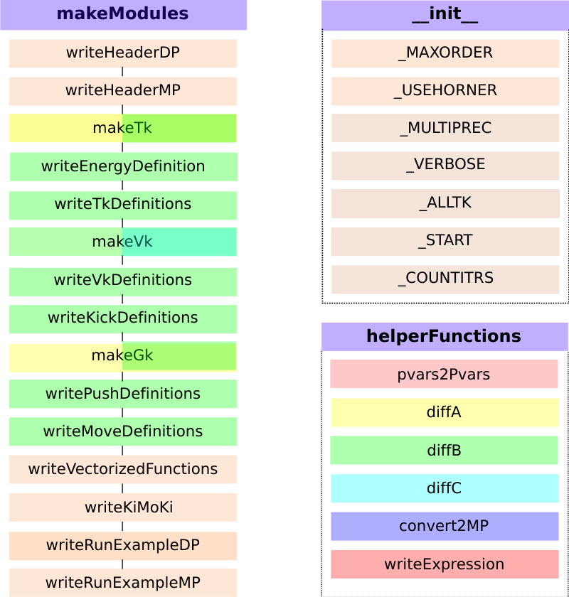
5.2 Brief description of the routines

$\circ$

makeModules(modname, V, qvars, pvars[, kwargs])

This is the main subroutine, and the only one intended to by called by the user. Here modname is a “basename” of the generated files, V is a symbolic expression for the potential $V$ , qvars is a list of symbolic positions variables (generalized coordinates), and pvars is a list of symbolic momentum variables (canonically conjugate momenta). This routine takes a number of optional keyword arguments (kwargs) with defaults:
- PARAMS=None is a list of symbolic parameters used in $V$ .
- MAXORDER=8 is the maximum order of the generated solvers.
- DP=True is a switch which determines if code for normal (double) precision solvers should be generated.
- MP=False is a switch which determines if code for multiprecision solvers should be generated.
- VERBOSE=False is a switch which determines if messages from the code generation process should be written.
- ALLTK=False is a switch wich determines if code for calculating $T_{2}$ , $T_{4}$ , and $T_{6}$ is generated.
- COUNTITRS=False is a switch which determines if code for monitoring the iterative solution of (9a) is generated. This code makes a histogram of the number of iterations used for solutions.
$\circ$

diffA(V, qvars, pvars), diffB(V, V0, qvars), diffC(V, qvars)

These three functions implement respectively the operator $D$ defined in equation (10), the operator $\bar{D}$ defined in expressions (10), and the operator $\bar{D}_{3}$ defined in equation (12). Here V0 is a symbolic expression of the potential defining the model, while V can be any symbolic expression depending on qvars, pvars, and potential parameters params. The function diffA is used by the routines makeTk and makeGk; the function diffB is used by the routines makeTk, makeVk and makeGk; the function diffC is used by the routine makeVk.
$\circ$

writeExpression(outfile, expression), convert2MP(match)

The function writeExpression writes expression to outfile in python format. If a multiprecision version of the solver module is generated, the function convert2MP is used to assure that fractions are converted to multiprecision format. Optionally a polynomial expression can be converted to Horner form first (this is not recommended if expression depends on many variables, due to time and memory use).
$\circ$

writeHeaderDP(outfile, pvars, params),
writeHeaderMP(outfile, pvars, params)

These routines write the header part of respectively the double precision and multiprecision solver modules. Some important solver module variables are defined here, with defaults:
- tau = 1/10 (DP), tau = 1/mpf(1000) (MP).
  
  The timestep $\tau$ used by the solvers.
- epsilon = 1/10**12 (DP), epsilon = 1/mpf(10**20) (MP).
  
  The accuracy to which (9a) must be solved. We have observed that the symplectic preserving property of the solvers is lost when epsilon is too large, but it must be somewhat larger than the numerical precision used.
- order = MAXORDER. Which order of solver to use, setting order larger than maxorder (see below) has no effect.
- params. A list of the symbolic potential parameters; these parameters must be set before starting a solution.
- maxorder = MAXORDER. The maximum order of generated solvers. Must not be changed by the user.
- dim. The number of phase space variables. Must not be changed.
- itrs[20]. A histogram of how many iterations are used to solve (9a). Exists only if COUNTITRS is set to True. Must not be changed by the user.
$\circ$

makeTk(V0, qvars, pvars)

Calculates the contributions $T_{0}$ , $T_{2}$ , $T_{4}$ , and $T_{6}$ to $T_{\text{eff}}$ , cf. (7a), using explicit expressions in (11). $T_{0}$ is used by the routine writeEnergyDefinition; $T_{2}$ , $T_{4}$ , and $T_{6}$ by the routine writeTkDefinitions. $T_{2}$ , $T_{4}$ , and $T_{6}$ are computed only when the optiononal parameter ALLTK=True, otherwise they are set to 0.
$\circ$

writeEnergyDefinition(outfile, qvars, pvars, T0, V0)

Writes the definition of the function energy(z), which evaluates the energy $T_{0}(\bm{p})+V_{0}(\bm{q})$ , cf. equation (2), at the phase space point $z\equiv(\bm{q},\bm{p})$ .
$\circ$

writeTkDefinitions(outfile, qvars, pvars, Tk)

Writes the definitions of the functions T2(z), T4(z) and T6(z), using the symbolic expressions in the list Tk calculated by makeTk.
$\circ$

makeVk(V0, qvars)

Calculates the contributions $V_{2}$ , $V_{4}$ , and $V_{6}$ to $V_{\text{eff}}$ , cf. equation (7b), using explicit expressions in equation (11). $V_{2}$ , $V_{4}$ , and $V_{6}$ are used by the routines writeVkDefinitions and writeKickDefinitions.
$\circ$

writeVkDefinitions(outfile, qvars, Vk)

Writes the definitions of the functions V2(q), V4(q) and V6(q), using the symbolic expressions in the list Vk calculated by makeVk.
$\circ$

writeKickDefinitions(outfile, qvars, Vk)

Calculates the symbolic expressions $-{\partial V_{\text{eff}}}/{\partial q^{a}}$ , cf. equation (3), using symbolic expressions in the list Vk calculated by makeVk. These expressions are used to define the functions kick $a$ (z) used in the kick-steps of the solvers.
$\circ$

makeGk(V0, qvars, Pvars)

Calculates the contributions $G_{3}$ , $G_{4}$ , …, $G_{8}$ to the generation function $G(\bm{q},\bm{P};\tau)$ , cf. equation (8), using the explicit expressions in equation (13). $G_{3}$ , $G_{4}$ , …, $G_{8}$ are used by writePushDefinitions and writeMoveDefinitions.
$\circ$

writePushDefinitions(outfile, qvars, Pvars, Gk)

Calculates the symbolic expressions ${\partial G}/{\partial q^{a}}$ , cf. equation (9a), using symbolic expressions in the list Gk calculated by makeGk. These expressions are used to define the functions push $a$ (z) used in the push-steps of the solvers.
$\circ$

writeMoveDefinitions(outfile, qvars, Pvars, Gk)

Calculates the symbolic expressions ${\partial G}/{\partial P_{a}}$ , cf. equation (9b), using symbolic expressions in the list Gk calculated by makeGk. These expressions are used to define the functions move $a$ (z) used in the move-steps of the solver(s).
$\circ$

writeVectorizedDefinitions(outfile, qvars, Pvars)

Writes definitions of functions vecKicks(idx, z), vecPushes(idx, z), and vecMoves(idx, z), simulating parallel evaluation of kick $a$ (z), push $a$ (z), and move $a$ (z), for all $a$ in the list idx. We don’t think parallel evaluation is actually achieved⁴⁴ 4 This depends on how the numpy.vectorize function is implemented.; hence presently this is only syntactic sugar simplifying the main solver routine, kiMoKi(z).
$\circ$

writeKiMoKi(outfile)

Writes the definition of the main algorithm of the solver module, kiMoKi(z). The routine kiMoKi(z) processes the kick-push-move-kick substeps of a full timestep, including the iterative solution of equation (9a).
$\circ$

writeRunExampleDP(outfile, modname, qvars, pvars, params),
writeRunExampleMP(outfile, modname, qvars, pvars, params)

Writes a simple example program illustrating how to use the solver module. Some routines of this program solves the Hamilton’s equation over a time interval, with random initial conditions and parameters (which most likely must first be manually changed to sensible values), and writes a plot of the solution to a pdf file. Other routines check how well energy is conserved by the solver, for a set of timesteps, and writes a plot of the energy errors to another pdf file.

Figure 11: This figure illustrates the runfile example. Normally the runfile generates two figure files in .png format (this can easily be changed to .pdf format by the user). The runfile also generate several intermediate files. Their names begin with the symbol #. These files are normally deleted after use (this can easily be changed by the user).

6 Concluding remarks

In this paper we have demonstrated that the proposed extensions of the standard Störmer-Verlet symplectic integration scheme can be implemented numerically, and that the implemented code behave as expected with respect to accuracy. Here we have not focused on time or memory efficiency of the generated code, which may be viewed as a reference implementation known to work correctly. We have experienced this to be a good starting point for manual implementation of more efficient code for large, structured systems, f.i. the Fermi-Pasta-Ulam-Tsingou type lattice models studied in [9], and molecular dynamics type simulations studied in [12]. Code for the latter systems are quite straightforward to implement using NumPy arrays [13], which also leads to efficient working code.

It is also straightforward to modify our program to generate code in other computer languages.

Acknowledgements

We thank professor Anne Kværnø for useful discussions, helpful feedbacks, and careful proofreading. We also acknowledge support provided by Statoil via Roger Sollie, through a professor II grant in Applied mathematical physics.

References

[1] J. M. Sanz-Serna, M. P. Calvo, Numerical Hamiltonian Problems, Chapman and Hall, (1994)
[2] R. I. McLachlan, G. R. Quispel, Splitting methods, Acta Numerica, 341–434 (2002)
[3] E. Hairer, Ch. Lubich, G. Wanner, Geometric Numerical Integrators. Structure-Preserving Algorithms for Ordinary Differential Equations, Springer-Verlag, 2nd edition (2006).
[4] I. Newton, Philosophiæ Naturalis Principia Mathematica (1687).
[5] Richard Feynman, The Character of Physical Law, p. 43, Penguin Science series, Penguin Books, London (1992).
[6] C. Störmer, Méthode d’intégration numérique des équations différentielles ordinares, C.R. Congress Internat. Stassbourg 1920, 243–257 (1921).
[7] Loup Verlet, Computer “Experiments” on Classical Fluids. I. Thermodynamical Properties of Lennard-Jones Molecules, Physical Review 159, 98-103 (1967).
[8] H. Goldstein, Classical Mechanics (3rd ed.), Addison-Wesley, 589–598 (2001).
[9] A. Mushtaq, A. Kværnø, K. Olaussen, Higher order Geometric Integrators for a class of Hamiltonian systems, International Journal of Geometric Methods in Modern Physics, 11, 1450009-1–1450009-20 (2014). DOI: 10.1142/S0219887814500091, arXiv.org:1301.7736
[10] A. Mushtaq, A. Kværnø, K. Olaussen, Systematic Improvement of Splitting Methods for the Hamilton Equations, Proceedings for the World Congress on Engineering, London July 4–6, Vol I, 247-251, (2012). arXiv.org:1204.4117v1.
[11] M. Abramowitz and I.S. Segun, Handbook of Mathematical Functions, Ch. 16, Dover Publications (1968)
[12] A. Mushtaq, A. Noreen, K. Olaussen, and R. Sollie, Ensemble and Occupation Time Probabilities, and the Rôle of Identical Particles, in preparation (2013).
[13] S. van der Walt, S.C. Colbert, G. Varoquaux, The NumPy Array: A Structure for Efficient Numerical Computation, Computing in Science & Engineering 13, 22–30 (2011).