A Fast Hadamard Transform for Signals with Sub-linear Sparsity in the Transform Domain

Robin Scheibler Saeid Haghighatshoar Martin Vetterli ^†^†thanks: R. Scheibler, S. Haghighatshoar and Martin Vetterli are with the School of Computer and Communication Sciences École Polytechnique Fédérale de Lausanne (EPFL), CH-1015 Lausanne, Switzerland.^†^†thanks: Email: {robin.scheibler, saeid.haghighatshoar, martin.vetterli}@epfl.ch^†^†thanks: The research of Robin Scheibler was supported by ERC Advanced Investigators Grant: Sparse Sampling: Theory, Algorithms and Applications SPARSAM no. $247006$.^†^†thanks: A short version of this paper was presented at the 51st Annual Allerton Conference on Communication, Control, and Computing, Monticello, 2013.

Abstract

A new iterative low complexity algorithm has been presented for computing the Walsh-Hadamard transform (WHT) of an $N$ dimensional signal with a $K$ -sparse WHT, where $N$ is a power of two and $K=O(N^{\alpha})$ , scales sub-linearly in $N$ for some $0<\alpha<1$ . Assuming a random support model for the non-zero transform domain components, the algorithm reconstructs the WHT of the signal with a sample complexity $O(K\log_{2}(\frac{N}{K}))$ , a computational complexity $O(K\log_{2}(K)\log_{2}(\frac{N}{K}))$ and with a very high probability asymptotically tending to $1$ .

The approach is based on the subsampling (aliasing) property of the WHT, where by a carefully designed subsampling of the time domain signal, one can induce a suitable aliasing pattern in the transform domain. By treating the aliasing patterns as parity-check constraints and borrowing ideas from erasure correcting sparse-graph codes, the recovery of the non-zero spectral values has been formulated as a belief propagation (BP) algorithm (peeling decoding) over a sparse-graph code for the binary erasure channel (BEC). Tools from coding theory are used to analyze the asymptotic performance of the algorithm in the “very sparse” ( $\alpha\in(0,\frac{1}{3}]$ ) and the “less sparse” ( $\alpha\in(\frac{1}{3},1)$ ) regime.

Index Terms:

Walsh-Hadamard, Transform, sparse, sparse FFT, sub-linear, peeling decoder.

I Introduction

The fast Walsh-Hadamard transform (WHT) is a well-known signal processing tool with application in areas as varied as image compression and coding [1], spreading sequence for multi-user transmission in cellular networks (CDMA) [2], spectroscopy [3] as well as compressed sensing [4]. It has also nice properties studied in different areas of mathematics [5]. Its recursive structure, similar to the famous fast Fourier transform (FFT) algorithm for computing the discrete Fourier transform (DFT) of the signal, allows a fast computation with complexity $O(N\log_{2}(N))$ in the dimension of the signal $N$ [6, 7].

A number of recent publications have addressed the particular problem of computing the DFT of an $N$ dimensional signal under the assumption of $K$ -sparsity of the signal in the frequency domain [8, 9, 10, 11, 12]. In particular, it has been shown that the well known computational complexity $O(N\log_{2}(N))$ of the FFT algorithm can be strictly improved. Such algorithms are generally known as sparse FFT (sFFT) algorithms. The authors in [13] by extending the results of [12], gave a very low complexity algorithm for computing the 2D-DFT of a $\sqrt{N}\times\sqrt{N}$ signal. In a similar line of work, based on the subsampling property of the DFT in the time domain resulting in aliasing in the frequency domain, the authors in [14, 15] developed a novel low complexity iterative algorithm to recover the non-zero frequency elements using ideas from sparse-graph codes [16].

In this paper, we develop a fast algorithm to compute the WHT of data sparse in the Hadamard domain. We first develop some useful properties of the WHT, specially the subsampling and the modulation property, that will later play a vital role in the development the algorithm. In particular, we show the subsampling in time domain allows to induce a well-designed aliasing pattern over the transform domain components. In other words, it is possible to obtain a linear combination of a controlled collection of transform domain components (aliasing), which creates interference between the non-zero components if more than one of them are involved in the induced linear combination. Similar to [15] and borrowing ideas from sparse-graph codes, we construct a bipartite graph by considering the non-zero values in the transform domain as variable nodes and interpreting any induced aliasing pattern as a parity check constraint over the variables in the graph. We analyze the structure of the resulting graph assuming a random support model for the non-zero coefficients in the transform domain. Moreover, we give an iterative peeling decoder to recover those non-zero components. In a nutshell, our proposed sparse fast Hadamard transform (SparseFHT) consists of a set of deterministic linear hash functions (explicitly constructed) and an iterative peeling decoder that uses the hash outputs to recover the non-zero transform domain variables. It recovers the $K$ -sparse WHT of the signal in sample complexity (number of time domain samples used) $O(K\log_{2}(\frac{N}{K}))$ , total computational complexity $O(K\log_{2}(K)\log_{2}(\frac{N}{K}))$ and with a high probability approaching $1$ asymptotically, for any value of $K$ .

Notations and Preliminaries: For $m$ an integer, the set of all integers $\{0,1,\dots,m-1\}$ is denoted by $[m]$ . We use the small letter $x$ for the time domain and the capital letter $X$ for the transform domain signal. For an $N$ dimensional real-valued vector $v$ , with $N=2^{n}$ a power of two, the $i$ -th components of $v$ is equivalently represented by $v_{i}$ or $v_{i_{0},i_{1},\ldots,i_{n-1}}$ , where $i_{0},i_{1},\dots,i_{n-1}$ denotes the binary expansion of $i$ with $i_{0}$ and $i_{n-1}$ being the least and the most significant bits. Also sometimes the real value assigned to $v_{i}$ is not important for us and by $v_{i}$ we simply mean the binary expansion associated to its index $i$ , however, the distinction must be clear from the context. $\mathbb{F}_{2}$ denotes the binary field consisting of $\{0,1\}$ with summation and multiplication modulo $2$ . We also denote by $\mathbb{F}_{2}^{n}$ the space of all $n$ dimensional vectors with binary components and addition of the vectors done component wise. The inner product of two $n$ dimensional binary vectors $u,v$ is defined by $\left\langle u\,,\,v\right\rangle=\sum_{t=0}^{n-1}u_{t}v_{t}$ with arithmetic over $\mathbb{F}_{2}$ although $\left\langle\,,\,\right\rangle$ is not an inner product in exact mathematical sense, for example, $\left\langle u\,,\,u\right\rangle=0$ for any $u\in\mathbb{F}_{2}^{n}$ .

For a signal $X\in\mathbb{R}^{N}$ , the support of $X$ is defined as $\operatorname{supp}(X)=\{i\in[N]:X_{i}\neq 0\}$ . The signal $X$ is called $K$ -sparse if $|\operatorname{supp}(X)|=K$ , where for a set $A\subset[N]$ , $|A|$ denotes the cardinality or the number of elements of $A$ . For a collection of $N$ dimensional signals ${\cal S}_{N}\subset\mathbb{R}^{N}$ , the sparsity of ${\cal S}_{N}$ is defined as $K_{N}=\max_{X\in{\cal S}_{N}}|\operatorname{supp}(X)|$ .

Definition 1.

A class of signals of increasing dimension $\{{\cal S}_{N}\}_{N=1}^{\infty}$ has sub-linear sparsity if there is $0<\alpha<1$ and some $N_{0}\in\mathbb{N}$ such that for all $N>N_{0}$ , $K_{N}\leq N^{\alpha}$ . The value $\alpha$ is called the sparsity index of the class.

II Main Results

Let us first describe the main result of this work in the following theorem.

Theorem 1.

Let $0<\alpha<1$ , $N=2^{n}$ a power of two and $K=N^{\alpha}$ . Let $x\in\mathbb{R}^{N}$ be a time domain signal with a WHT $X\in\mathbb{R}^{N}$ . Assume that $X$ is a $K$ -sparse signal in a class of signals with sparsity index $\alpha$ whose support is uniformly at random selected among all possible ${N\choose K}$ subsets of $[N]$ of size $K$ . For any value of $\alpha$ , there is an algorithm that can compute $X$ and has the following properties:

1.

Sample complexity: The algorithm uses $CK\log_{2}(\frac{N}{K})$ time domain samples of the signal $x$ . $C$ is a function of $\alpha$ and $C\leq(\frac{1}{\alpha}\vee\frac{1}{1-\alpha})+1$ , where for $a,b\in\mathbb{R}_{+}$ , $a\vee b$ denotes the maximum of $a$ and $b$ .
2.

Computational complexity: The total number of operations in order to successfully decode all the non-zero spectral components or announce a decoding failure is $O(CK\log_{2}(K)\log_{2}(\frac{N}{K}))$ .
3.

Success probability: The algorithm correctly computes the $K$ -sparse WHT $X$ with very high probability asymptotically approaching $1$ as $N$ tends to infinity, where the probability is taken over all random selections of the support of $X$ .

Remark 1.

To prove Theorem 1, we distinguish between the very sparse case ( $0<\alpha\leq\frac{1}{3}$ ) and less sparse one ( $\frac{1}{3}<\alpha<1$ ). Also, we implicitly assume that the algorithm knows the value of $\alpha$ which might not be possible in some cases. As we will see later if we know to which regime the signal belongs and some bounds on the value of the $\alpha$ , it is possible to design an algorithm that works for all those values of $\alpha$ . However, the sample and computational complexity of that algorithm might increase compared with the optimal one that knows the value of $\alpha$ . For example, if we know that the signal is very sparse, $\alpha\in(0,\alpha^{*}]$ with $\alpha^{*}\leq\frac{1}{3}$ , it is sufficient to design the algorithm for $\alpha^{*}$ and it will work for all signals with sparsity index less that $\alpha^{*}$ . Similarly, if the signal is less sparse with a sparsity index $\alpha\in(\frac{1}{3},\alpha^{*})$ , where $\alpha^{*}<1$ , then again it is sufficient to design the algorithm for $\alpha^{*}$ and it will automatically work for all $\alpha\in(\frac{1}{3},\alpha^{*})$ .

Remark 2.

In the very sparse regime ( $0<\alpha\leq\frac{1}{3}$ ), we prove that for any value of $\alpha$ the success probability of the optimally designed algorithm is at least $1-O(1/K^{3(C/2\,-1)})$ , with $C=[\frac{1}{\alpha}]$ where for $u\in\mathbb{R}_{+}$ , $[u]=\max\{n\in\mathbb{Z}:n\leq u\}$ . It is easy to show that for every value of $\alpha\in(0,\frac{1}{3})$ the success probability can be lower bounded by $1-O(N^{-\frac{3}{8}})$ .

III Walsh-Hadamard Transform and its Properties

Let $x$ be an $N=2^{n}$ dimensional signal indexed with elements $m\in\mathbb{F}_{2}^{n}$ . The $N$ dimensional WHT of the signal $x$ is defined by

X_{k}=\frac{1}{\sqrt{N}}\sum_{m\in\mathbb{F}_{2}^{n}}(-1)^{\left\langle k\,,\,m\right\rangle}x_{m},

where $k\in\mathbb{F}_{2}^{n}$ denote the corresponding binary index of the transform domain component. Also, throughout the paper, borrowing some terminology from the DFT, we call transform domain samples $X_{k},k\in\mathbb{F}_{2}^{n}$ frequency or spectral domain components of the time domain signal $x$ .

III-A Basic Properties

This subsection is devoted to reviewing some of the basic properties of the WHT. Some of the properties are not directly used in the paper and we have included them for the sake of completeness. They can be of independent interest. The proofs of all the properties are provided in Appendix A.

Property 1 (Shift/Modulation).

Let $X_{k}$ be the WHT of the signal $x_{m}$ and let $p\in\mathbb{F}_{2}^{n}$ . Then

\displaystyle{x_{m+p}\quad\overset{\text{WHT}}{\longleftrightarrow}\quad X_{k}(-1)^{\left\langle p\,,\,k\right\rangle}}.

The next property is more subtle and allows to partially permute the Hadamard spectrum in a specific way by applying a corresponding permutation in the time domain. However, the collection of all such possible permutations is limited. We give a full characterization of all those permutations. Technically, this property is equivalent to finding permutations $\pi_{1},\pi_{2}:[N]\to[N]$ with corresponding permutation matrices $\Pi_{1},\Pi_{2}$ such that

\Pi_{2}H_{N}=H_{N}\Pi_{1},

(1)

where $H_{N}$ is the Hadamard matrix of order $N$ and where the permutation matrix corresponding to a permutation $\pi$ is defined by $(\Pi)_{i,j}=1$ if and only if $\pi(i)=j$ , and zero otherwise. The identity (1) is equivalent to finding a row permutation of $H_{N}$ that can be equivalently obtained by a column permutation of $H_{N}$ .

Property 2.

All of the permutations satisfying (1) are described by the elements of

\operatorname{GL}(n,\mathbb{F}_{2})=\{A\in\mathbb{F}_{2}^{n\times n}\,|\,A^{-1}\ \text{exists}\},

the set of $n\times n$ non-singular matrices with entries in $\mathbb{F}_{2}$ .

Remark 3.

The total number of possible permutations in Property 2, is $\prod_{i=0}^{n-1}(N-2^{i})$ , which is a negligible fraction of all $N!$ permutation over $[N]$ .

Property 3 (Permutation).

Let $\Sigma\in\operatorname{GL}(n,\mathbb{F}_{2})$ . Assume that $X_{k}$ is the WHT of the time domain signal $x_{m}$ . Then

x_{\Sigma m}\quad\overset{\text{WHT}}{\longleftrightarrow}\quad X_{\Sigma^{-T}k}.

Remark 4.

Notice that any $\Sigma\in\operatorname{GL}(n,\mathbb{F}_{2})$ is a bijection from $\mathbb{F}_{2}^{n}$ to $\mathbb{F}_{2}^{n}$ , thus $x_{\Sigma m}$ is simply a vector obtained by permuting the initial vector $x_{m}$ .

The last property is that of downsampling/aliasing. Notice that for a vector $x$ of dimension $N=2^{n}$ , we index every components by a binary vector of length $n$ , namely, $x_{m_{0},m_{1},\dots,m_{n-1}}$ . To subsample this vector along dimension $i$ , we freeze the $i$ -th component of the index to either $0$ or $1$ . For example, $x_{0,m_{1},\dots,m_{n-1}}$ is a $2^{n-1}$ dimensional vector obtained by subsampling the vector $x_{m}$ along the first index.

Property 4 (Downsampling/Aliasing).

Suppose that $x$ is a vector of dimension $N=2^{n}$ indexed by the elements of $\mathbb{F}_{2}^{n}$ and assume that $B=2^{b}$ , where $b\in\mathbb{N}$ and $b<n$ . Let

\Psi_{b}=\left[\,\mathbf{0}_{b\times(n-b)}\ I_{b}\,\right]^{T},

(2)

be the subsampling matrix freezing the first $n-b$ components in the index to $0$ . If $X_{k}$ is the WHT of $x$ , then

x_{\Psi_{b}m}\quad\overset{\text{WHT}}{\longleftrightarrow}\quad\sqrt{\frac{B}{N}}\sum_{j\in\mathcal{N}\left(\Psi_{b}^{T}\right)}X_{\Psi_{b}k+j},

where $x_{\Psi_{b}m}$ is a $B$ dimensional signal labelled with $m\in\mathbb{F}_{2}^{b}$ .

Notice that Property 4 can be simply applied for any matrix $\Psi_{b}$ that subsamples any set of indices of length $b$ not necessarily the $b$ last ones.

Remark 5.

The group $\mathbb{F}_{2}^{n}$ can be visualized as the vertices of the $n$ -dimensional hypercube. The downsampling property just explained implies that downsampling along some of the dimensions in the time domain is equivalent to summing up all of the spectral components along the same dimensions in the spectral domain. This is illustrated visually in Fig. 1 for dimension $n=3$ .

Fig. 1: Illustration of the downsampling property on a hypercube for

N=2^{3}

. The two cubes are the time-domain and Hadamard-domain signals on the left and right, respectively. We decide to drop all nodes whose third coordinate is ’1’. We illustrate this by adding an ’

\times

’ on the edges connecting these vertices through the third coordinate. This is equivalent to summing up vertices along the corresponding edges in the Hadamard domain.

Remark 6.

In a general downsampling procedure, one can replace the frozen indices by an arbitrary but fixed binary pattern. The only difference is that instead of summing the aliased spectral components, one should also take into account the suitable $\{+,-\}$ sign patterns, namely, we have

x_{\Psi_{b}m+p}\quad\overset{\text{WHT}}{\longleftrightarrow}\quad\sqrt{\frac{B}{N}}\sum_{j\in\mathcal{N}\left(\Psi_{b}^{T}\right)}(-1)^{\left\langle p\,,\,j\right\rangle}X_{\Psi_{b}k+j},

(3)

where $p$ is a binary vector of length $n$ with $b$ zeros at the end.

IV Hadamard Hashing Algorithm

By applying the basic properties of the WHT, one can design suitable hash functions in the spectral domain. The main idea is that one does not need to have access to the spectral values and the output of all hash functions can be simply computed by low complexity operations on the time domain samples of the signal.

Proposition 1 (Hashing).

Assume that $\Sigma\in\operatorname{GL}(n,\mathbb{F}_{2})$ and $p\in\mathbb{F}_{2}^{n}$ . Let $N=2^{n}$ , $b\in\mathbb{N}$ , $B=2^{b}$ and let $m,k\in\mathbb{F}_{2}^{b}$ denote the time and frequency indices of a $B$ dimensional signal and its WHT defined by

u_{\Sigma,p}(m)=\sqrt{\frac{N}{B}}\,x_{\Sigma\Psi_{b}m+p}.

Then, the length $B$ Hadamard transform of $u_{\Sigma,p}$ is given by

U_{\Sigma,p}(k)=\sum_{j\in\mathbb{F}_{2}^{n}\,|\,\mathcal{H}j=k}X_{j}\,(-1)^{\left\langle p\,,\,j\right\rangle},

(4)

where $\mathcal{H}$ is the index hashing operator defined by

\mathcal{H}=\Psi_{b}^{T}\Sigma^{T},

(5)

where $\Psi_{b}$ is as in (2). Note that the index of components in the sum (4) can be explicitely written as function of the bin index $k$

\displaystyle j=\Sigma^{-T}\Psi_{b}k+q,\qquad q\in\mathcal{N}(\mathcal{H}).

The proof simply follows from the properties 1, 3, and 4.

Based on Proposition 1, we give Algorithm 1 which computes the hashed Hadamard spectrum. Given an FFT-like fast Hadamard transform (FHT) algorithm, and picking $B$ bins for hashing the spectrum, Algorithm 1 requires $O(B\log B)$ operations.

Algorithm 1 FastHadamardHashing

(x,N,\Sigma,p,B)

0: Signal

x

of dimension

N=2^{n}

\Sigma

and

p

and given number of output bins

B=2^{b}

in a hash.

U

contains the hashed Hadamard spectrum of

x

u_{m}=x_{\Sigma\Psi_{b}m+p}

, for

m\in\mathbb{F}_{2}^{b}

U=\sqrt{\frac{N}{B}}\operatorname{FastHadamard}(u_{m},B)

IV-A Properties of Hadamard Hashing

In this part, we review some of the nice properties of the hashing algorithm that are crucial for developing an iterative peeling decoding algorithm to recover the non-zero spectral values. We explain how it is possible to identify collisions between the non-zero spectral coefficients that are hashed to the same bin and also to estimate the support of non-colliding components.

Let us consider $U_{\Sigma,p}(k)$ for two cases: $p=0$ and some $p\neq 0$ . It is easy to see that in the former $U_{\Sigma,p}(k)$ is obtained by summing all of the spectral variables hashed to bin $k$ – those whose index $j$ satisfies $\mathcal{H}j=k$ – whereas in the latter the same variables are added together weighted by $(-1)^{\left\langle p\,,\,j\right\rangle}$ . Let us define the following ratio test

r_{\Sigma,p}(k)=\frac{U_{\Sigma,p}(k)}{U_{\Sigma,0}(k)}.

When the sum in $U_{\Sigma,p}(k)$ contains only one non-zero component, it is easy to see that $|r_{\Sigma,p}(k)|=1$ for ‘any value’ of $p$ . However, if there is more than one component in the sum, under a very mild assumption on the the non-zero coefficients of the spectrum (i.e. they are jointly sampled from a continuous distribution), one can show that $|r_{\Sigma,p}(k)|\neq 1$ for at least some values of $p$ . In fact, $n-b$ well-chosen values of $p$ allow to detect whether there is only one, or more than one non-zero components in the sum.

When there is only one $X_{j^{\prime}}\neq 0$ hashed to the bin $k$ ( $h_{\Sigma}(j^{\prime})=k$ ), the result of the ratio test is precisely $1$ or $-1$ , depending on the value of the inner product between $j^{\prime}$ and $p$ . In particular, we have

\left\langle p\,,\,j^{\prime}\right\rangle=\mathds{1}_{\left\{r_{\Sigma,p}(k)<0\right\}},

(6)

where $\mathds{1}_{\left\{t<0\right\}}=1$ if $t<0$ , and zero otherwise. Hence, if for $n-b$ well-chosen values of $p$ , the ratio test results in $1$ or $-1$ , implying that there is only one non-zero spectral coefficient in the corresponding hash bin, by some extra effort it is even possible to identify the position of this non-zero component. We formalize this result in the following proposition proved in Appendix B.

Proposition 2 (Collision detection / Support estimation).

Let $\Sigma\in\operatorname{GL}(n,\mathbb{F}_{2})$ and let $\sigma_{i},i\in[n]$ denote the columns of $\Sigma$ .

1.

If for all $d\in[n-b]$ , $|r_{\Sigma,\sigma_{d}}(k)|=1$ then almost surely there is only one non-zero spectral value in the bin indexed by $k$ . Moreover, if we define

$\hat{v}_{d}=\begin{cases}\mathds{1}_{\left\{r_{\Sigma,\sigma_{d}}(k)<0\right\}}&d\in[n-b],\\ 0&\text{otherwise,}\end{cases}$

the index of the unique non-zero coefficient is given by

$j=\Sigma^{-T}(\Psi_{b}\,k+\hat{v}).$ (7)
2.

If there exists a $d\in[n-b]$ such that $|r_{\Sigma,\sigma_{d}}(k)|\neq 1$ then the bin $k$ contains more than one non-zero coefficient.

Fig. 2: On the left, bipartite graph representation of the WHT for

N=8

and

K=3

. On the right, the underlying bipartite graph after applying

C=2

different hashing produced by plugging

\Sigma_{1}

\Sigma_{2}

in (5) with

B=4

. The variable nodes (

\bullet

) are the non-zero spectral values to be recovered. The white check nodes (

\square

) are the original time-domain samples. The colored squares are new check nodes after applying Algorithm 1.

Fig. 3: A block diagram of the SparseFHT algorithm in the time domain. The downsampling plus small size low complexity FHT blocks compute different hash outputs. Delay blocks denote an index shift by

\sigma_{i}

before hashing. The S/P and P/S are serial-parallel and parallel-serial blocks to emphasize that the FHT operates on the whole signal at once. The collision detection/support estimation block implements Proposition 2 to identify if there is a collision. Index

i

is not valid when there is a collision.

V Sparse Fast Hadamard Transform

In this section, we give a brief overview of the main idea of Sparse Fast Hadamard Transform (SparseFHT). In particular, we explain the peeling decoder which recovers the non-zero spectral components and analyze its computational complexity.

V-A Explanation of the Algorithm

Assume that $x$ is an $N=2^{n}$ dimensional signal with a $K$ -sparse WHT $X$ , where $K=O(N^{\alpha})$ scales sub-linearly with $N$ with index $\alpha$ . As $H_{N}^{-1}=H_{N}$ , taking the inner product of the vector $X$ with the $i$ -th row of the Hadamard matrix $H_{N}$ gives the time domain sample $x_{i}$ . Using the terminology of Coding theory, it is possible to consider the spectral components $X$ as variables nodes (information bits in coding theory) where the inner product of the $i$ -th row of $H_{N}$ is like a parity check constraint on $X$ . For example, the first row of the Hadamard matrix is the all-one vector which implies that the sum of all of the components of $X$ must be equal to the first time domain sample. A similar interpretation holds for the other rows. Thus, the WHT can be imagined as a code over a bipartite graph. With this picture in mind, one can consider the recovery of the non-zero spectral values as a decoding problem over this bipartite graph. If we consider the WHT, it is easy to see that the induced bipartite graph on the non-zero spectral values is a complete (dense) bipartite graph because any variable node is connected to all of the check nodes as has been depicted in the left part of Fig. 2, where $\{X_{1},X_{8},X_{11}\}$ are the only non-zero variables in the spectral domain and each check constraint correspond to the value of a time domain sample. It is also implicitly assumed that one knows the support of $X$ , $\{1,8,11\}$ in our case. At the moment, it is not clear how one can obtain the position of the non-zero variables. As we will explain, in the final version of the algorithm this can be done by using Proposition 2.

For codes on bipartite graphs, there is a collection of low complexity belief propagation algorithms to recover the variable nodes given the value of check nodes. Most of these algorithms perform well assuming the sparsity of the underlying bipartite graph. Unfortunately, the graph corresponding to WHT is dense, and probably not suitable for any of these belief propagation algorithms to succeed.

As explained in Section IV, by subsampling the time domain components of the signal it is possible to hash the spectral components in different bins as depicted for the same signal $X$ in the right part of Fig. 2. The advantage of the hashing operation must be clear from this picture. The idea is that hashing ‘sparsifies’ the underlying bipartite graph. It is also important to notice that in the bipartite graph induced by hashing, one can obtain all of the values of parity checks (hash outputs) by using low complexity operations on a small set of time domain samples as explained in Proposition 1.

We propose the following iterative algorithm to recover the non-zero spectral variables over the bipartite graph induced by hashing. The algorithm first tries to find a degree one check node. Using the terminology of [15], we call such a check node a singleton. Using Proposition 2, the algorithm is able to find the position and the value of the corresponding non-zero component and, thus the algorithm can subtract (peel off) this variable from all other check nodes that are connected to it. In particular, after this operation the corresponding singleton check node gets value zero, namely, it is satisfied. Equivalently, we can update the underlying graph by removing the mentioned variable node from the graph along with all the edges connected to it. This creates an isolated (degree zero) check node which we call a zeroton. Also notice that by removing some of the edges from the graph, the degree of the associated checks decreases by one, thus there is a chance that another singleton be found.

The algorithm proceeds to peel off a singleton at a time until all of the check nodes are zeroton (decoding succeeds) or all of the remaining check nodes have degree greater than one (we call them multiton) and the algorithm fails to identify all of the non-zero spectral values.

A more detailed pseudo-code of the proposed iterative algorithm is given in Algorithm 2.

Algorithm 2 SparseFHT

(x,N,K,C,L,\mbox{\boldmath$\Sigma$})

0: Input signal

x

of length

N=2^{n}

. Sparsity

K

. Hash count

C

. Number of iterations of decoder

L

. Array

\Sigma

C

matrices in

\operatorname{GL}(n,\mathbb{F}_{2})

\Sigma_{c}=[\sigma_{c,1}\,|\,\cdots\,|\,\sigma_{c,n}]

\sigma_{c,i}\in\mathbb{F}_{2}^{n}

X

contains the sparse Hadamard spectrum of

x

B=O(K)

D=n-b+1

for

c=1,\ldots,C

U_{c,0}=\operatorname{FastHadamardHashing}(x,N,\Sigma_{c},0,B)

for

d=1,\ldots,D

U_{c,d}=\operatorname{FastHadamardHashing}(x,N,\Sigma_{c},\sigma_{c,d},B)

end for

for

l=1,\ldots,L

for

c=1,\ldots,C

for

k=0,\ldots,B-1

U_{c,0,k}=0

then

continue to next

k

end if

\hat{v}\leftarrow 0

for

d=1,\ldots,D

U_{c,d,k}/U_{c,0,k}=-1

then

\hat{v}_{d-1}\leftarrow 1

else if

U_{c,d,k}/U_{c,0,k}\neq 1

then

continue to next

k

end if

end for

i\leftarrow\Sigma_{c}^{-T}(\Psi_{b}\,k+\hat{v})

X_{i}\leftarrow U_{c,0,k}

for

c^{\prime}=1,\ldots,C

j\leftarrow\Psi_{b}^{T}\Sigma_{c^{\prime}}^{T}\,i

U_{c^{\prime},0,j}\leftarrow U_{c^{\prime},0,j}-X_{i}

for

d^{\prime}=1,\ldots,D

U_{c^{\prime},d^{\prime},j}\leftarrow U_{c^{\prime},d^{\prime},j}-X_{i}(-1)^{\left\langle\sigma_{c^{\prime},d^{\prime}}\,,\,i\right\rangle}

end for

V-B Complexity Analysis

Figure 3 shows a full block diagram of the SparseFHT algorithm. Using this block diagram, it is possible to prove part $1$ and $2$ of Theorem 1 about the sample and the computational complexity of the SparseFHT algorithm. The proof of the last part of Theorem 1, regarding the success probability of the algorithm, is the subject of Sections VI and VII for the very and less sparse regimes, respectively.

Computational Complexity: As will be further clarified in Sections VI and VII, depending on the sparsity index of the signal $\alpha$ , we will use $C$ different hash blocks, where $C\leq(\frac{1}{\alpha}\vee\frac{1}{1-\alpha})+1$ each with $B=2^{b}$ different output bins. We always select $B=K$ to keep the average number of non-zero components per bin $\beta=\frac{K}{B}$ equal to $1$ . This implies that computing the hash outputs via an FHT block of size $B$ needs $B\log_{2}(B)$ operations which assuming $K=B$ , has a computational complexity $K\log_{2}(K)$ . Moreover, we need to compute any hash output with $n-b=\log_{2}(\frac{N}{B})$ different shifts in order to do collision detection/support estimation, thus, the computational cost for each hash is $K\log_{2}(K)\log_{2}(\frac{N}{K})$ . As we need to compute $C$ different hash blocks, the total computational complexity for each iteration will be $CK\log_{2}(K)\log_{2}(\frac{N}{K})$ . We will explain later that the algorithm terminates in a fixed number of iterations independent of the value of $\alpha$ and the dimension of the signal $N$ . Therefore, the total computational complexity of the algorithm will be $O(CK\log_{2}(K)\log_{2}(\frac{N}{K}))$ .

Sample Complexity: Assuming $K=B$ , computing each hash with $n-b$ different shifts needs $K\log_{2}(\frac{N}{K})$ time domain samples. Therefore, the total sample complexity will be $CK\log_{2}(\frac{N}{K})$ .

VI Performance Analysis of the very Sparse Regime

In this section, we consider the very sparse regime, where $0<\alpha\leq\frac{1}{3}$ . In this regime, we show that assuming a random support model for non-zero spectral components and a careful design of hash functions, it is possible to obtain a random bipartite graph with variable nodes corresponding to non-zero spectral components and with check nodes corresponding to outputs of hash functions. We explicitly prove that asymptotically this random graph behaves similarly to the ensemble of LDPC bipartite graph. Running the peeling decoder to recover the spectral components is also equivalent to the belief propagation (BP) decoding for a binary erasure channel (BEC). Fortunately, there is a rich literature in coding theory about asymptotic performance of the BP decoder. Specially, it is possible to show that the error (decoding failure) probability can be asymptotically characterized by a ‘Density Evolution’ (DE) equation allowing a perfect analysis of the peeling decoder.

We use the following steps to rigorously analyze the performance of the decoder in the very sparse regime:

1.

We explain construction of suitable hash functions depending on the value of $\alpha\in(0,\frac{1}{3}]$ .
2.

We rigorously analyze the structure of the induced bipartite graph obtained by treating the non-zero spectral components as variable nodes and the output of hash functions as check nodes. In particular, we prove that the resulting graph is a fully random left regular bipartite graph similar to the regular LDPC ensemble. We also obtain variable and check degrees distribution polynomials for this graph.
3.

At every stage, the peeling decoder recovers some of the variable nodes, removing all the edges incident to those variable nodes. We use Wormald’s method given in [17] to prove the concentration of the number of unpeeled edges around its expected value, which we also characterize. Wormald’s method as exploited in [18], uses the differential equation approach to track the evolution of the number of edges in the underlying bipartite graph. Specifically, it shows that the number of edges at every step of the algorithm is very well concentrated around the solution of the associated differential equations.
4.

Wormald’s method gives a concentration bound to the number of remaining edges as far as their count is a fixed ratio $\gamma\in(0,1)$ of the initial edges in the graph. Another expander argument as in [18] is necessary to show that if the peeling decoder peels $1-\gamma$ ratio of the edges successfully, it can continue to peel off all the remaining edges with very high probability.

VI-A Hash Construction

For the very sparse regime, $0<\alpha\leq\frac{1}{3}$ , consider those values of $\alpha$ equal to $\frac{1}{C}$ for some positive integer $C\geq 3$ . We will explain later how to cover the intermediate values. For $\alpha=\frac{1}{C}$ , we will consider $C$ different hash functions as follows. Let $x$ be an $N$ dimensional time domain signal with a WHT $X$ , where $N=2^{n}$ and let $b=\frac{n}{C}$ . As we explained before, the components of the vector $X$ can be labelled by $n$ dimensional binary vector from $\mathbb{F}_{2}^{n}$ . We design $C$ different subsampling operator, where the $i$ -th one returns all of the variables with indices $i\,b$ up to $(i+1)b-1$ kept and the other indices set to zero. Using the terminology of Proposition 1, we let $\Sigma_{i}$ be the identity matrix with columns circularly shifted by $(i+1)b$ to the left. Then, the hash operator given by (5) is

\displaystyle\mathcal{H}_{i}=\Psi_{b}^{T}\Sigma_{i}^{T}=[\mathbf{0}_{b\times ib}\ I_{b}\ \mathbf{0}_{b\times(n-(i+1)b)}],

where $I_{b}$ is the identity matrix of order $b$ and $\Phi_{b}$ is defined in (2). To give further intuition about hash construction, let us label the elements of the vector $x$ with their binary representation $x_{0}^{n-1}\in\mathbb{F}_{2}^{n}$ . Equivalent to the $C$ different subsampling operators, we can consider functions $h_{i},i\in[C]$ where $h_{i}(x_{0}^{n-1})=(x_{i\,b},x_{i\,b+1},\dots,x_{i\,b+b-1})$ . The important point is that with this construction, the outputs of different $h_{i}$ depend on non overlapping portions of the labeling binary indices. In particular, labeling the transform domain components by $X_{0}^{n-1}\in\mathbb{F}_{2}^{n}$ and ignoring the multiplicative constants, it is seen from Equation (4) that every spectral component $X_{0}^{n-1}$ is hashed to the bin labelled with $h_{i}(X_{0}^{n-1})\in\mathbb{F}_{2}^{b}$ in hash $i$ .

In terms of complexity, to obtain the output of each hash bin, we only need to compute the WHT of a smaller subsampled signal of dimension $B$ . Note that by hash construction, $K=B$ which implies that all of the hash functions can be computed in $CK\log_{2}(K)$ operations. As we will explain later, we need at least $C=3$ hashes for the peeling algorithm to work successfully and that is the main reason why this construction works for $\alpha\leq\frac{1}{3}$ . For intermediate values of $\alpha$ , those not equal to $\frac{1}{C}$ for some integer $C$ , one can construct $[\frac{1}{\alpha}]$ hashes with $B=2^{[n\alpha]}$ output bins and one hash with smaller number of output bins, thus obtaining a computational complexity of order $(1+[\frac{1}{\alpha}])K\log_{2}(K)$ .

VI-B Random Bipartite Graph Construction

VI-B1 Random Support Model

For an $N$ dimensional signal $x\in\mathbb{R}^{N}$ , the support of $x$ is defined as $\operatorname{supp}(x)=\{i\in[N]:x_{i}\neq 0\}$ . The signal $x$ is called $K$ sparse if $|\operatorname{supp}(x)|=K$ , where for $A\subset[N]$ , $|A|$ denotes the cardinality of $A$ . For a given $(K,N)$ , $\text{RS1}(K,N)$ is the class of all stochastic signals whose support is uniformly at random selected from the set of all ${N\choose K}$ possible supports of size $K$ . We do not put any constraint on the non-zero components; they can be deterministic or random. Model RS1 is equivalent to selecting $K$ out of $N$ objects at random without replacement. If we assume that the selection of the indices for the support is done independently but with replacement, we obtain another model that we call $\text{RS2}(K,N)$ . In particular, if $V_{i},i\in[K]$ are i.i.d. random variables uniformly distributed over $[N]$ , a random support in $\text{RS2}(K,N)$ is given by the random set $\{V_{i}:i\in[K]\}$ . Obviously, the size of a random support in $\text{RS2}(K,N)$ is not necessarily fixed but it is at most $K$ . The following proposition, proved in Appendix C, shows that in the sub-linear sparsity regime, RS1 and RS2 are essentially equivalent.

Proposition 3.

Consider the random support model $\text{RS2}(K,N)$ , where $K=N^{\alpha}$ for some fixed $0<\alpha<1$ and let $H$ be the random size of the support set. Asymptotically as $N$ tends to infinity $\frac{H}{K}$ converges to $1$ in probability.

VI-B2 ‘Balls and Bins’ Model ${\cal G}(K,B,C)$

Consider $C$ disjoint sets of check nodes $S_{1},S_{2},\dots,S_{C}$ of the same size $|S_{i}|=B$ . A graph in the ensemble of random bipartite graphs ${\cal G}$ with $K$ variable nodes at the left and $C\times B$ check nodes $\cup_{i=1}^{C}S_{i}$ at the right is generated as follows. Each variable node $v$ in ${\cal G}$ , independently from other variable nodes, is connected to check nodes $\{s_{1},s_{2},\dots,s_{C}\}$ where $s_{i}\in S_{i}$ is uniformly at random selected from $S_{i}$ and selection of $s_{i}$ ’s are independent of one another. Every edge $e$ in ${\cal G}$ can be labelled as $(v,c)$ , where $v\in[K]$ is a variable node and $c$ is a check node in one of $S_{1},S_{2},\dots,S_{C}$ . For a variable node $v$ , the neighbors of $v$ denoted by ${\cal N}(v)$ consists of $C$ different check nodes connected to $v$ , each of them from a different $S_{i}$ . Similarly, for a check node $c\in\cup_{i=1}^{C}S_{i}$ , ${\cal N}(c)$ is the set of all variable nodes connected to $c$ .

By construction, all of the resulting bipartite graphs in the ensemble are left regular with variable degree $C$ but the check node degree is not fixed. During the construction, it might happen that two variable nodes have exactly the same neighborhood. In that case, we consider them as equivalent variables and keep only one of them and remove the other, thus the number of variable nodes in a graph from the ensemble ${\cal G}(K,B,C)$ might be less than $K$ .

This model is a variation of the Balls and Bins model, where we have $K$ balls, $C$ buckets of different color each containing $B$ bins and every ball selects one bin from each bucket at random independent of the other balls.

Here we also recall some terminology from graph theory that we will use later. A walk of size $\ell$ in graph ${\cal G}$ starting from a node $v\in[K]$ is a set of $\ell$ edges $e_{1},e_{2},\dots,e_{\ell}$ , where $v\in e_{1}$ and where consecutive edges are different, $e_{i}\neq e_{i+1}$ , but incident with each other $e_{i}\cap e_{i+1}\neq\emptyset$ . A directed neighborhood of an edge $e=(v,c)$ of depth $\ell$ is the induced subgraph in ${\cal G}$ consisting of all edges and associated check and variable nodes in all walks of size $\ell+1$ starting from $v$ with the first edge being $e_{1}=(v,c)$ . An edge $e$ is said to have a tree neighborhood of depth $\ell$ if the directed neighborhood of $e$ of depth $\ell$ is a tree.

VI-B3 Ensemble of Graphs Generated by Hashing

In the very sparse regime ( $0<\alpha<\frac{1}{3}$ ), in order to keep the computational complexity of the hashing algorithm around $O(K\log_{2}(K))$ , we constructed $C=\frac{1}{\alpha}$ different surjective hash functions $h_{i}:\mathbb{F}_{2}^{n}\to\mathbb{F}_{2}^{b}$ , $i\in[C]$ , where $b\approx n\alpha$ and where for an $x\in\mathbb{F}_{2}^{n}$ with binary representation $x_{0}^{n-1}$ , $h_{i}(x_{0}^{n-1})=(x_{i\,b},x_{i\,b+1},\dots,x_{i\,b+b-1})$ . We also explained that in the spectral domain, this operation is equivalent to hashing spectral the component labeled with $X_{0}^{n-1}\in\mathbb{F}_{2}^{n}$ into the bin labelled with $h_{i}(X_{0}^{n-1})$ . Notice that by this hashing scheme there is a one-to-one relation between a spectral element $X$ and its bin indices in different hashes $(h_{0}(X),h_{1}(X),\dots,h_{C-1}(X))$ .

Let $V$ be a uniformly distributed random variable over $\mathbb{F}_{2}^{n}$ . It is easy to check that in the binary representation of $V$ , $V_{0}^{n-1}$ are like i.i.d. unbiased bits. This implies that $h_{0}(V),h_{1}(V),\dots,h_{C-1}(V)$ will be independent from one another because they depend on disjoint subsets of $V_{0}^{n-1}$ . Moreover, $h_{i}(V)$ is also uniformly distributed over $\mathbb{F}_{2}^{b}$ .

Assume that $X_{1},X_{2},\dots,X_{K}$ are $K$ different variables in $\mathbb{F}_{2}^{n}$ denoting the position of non-zero spectral components. For these $K$ variables and hash functions $h_{i}$ , we can associate a bipartite graph as follows. We consider $K$ variable nodes corresponding to $X_{1}^{K}$ and $C$ different set of check nodes $S_{0},S_{1},\dots,S_{C-1}$ each of size $B=2^{b}$ . The check nodes in each $S_{i}$ are labelled by elements of $\mathbb{F}_{2}^{b}$ . For each variable $X_{i}$ we consider $C$ different edges connecting $X_{i}$ to check nodes labelled with $h_{j}(X_{i})\in S_{j}$ , $j\in[C]$ .

Proposition 4.

Let $h_{i}:\mathbb{F}_{2}^{n}\to\mathbb{F}_{2}^{b}$ , $i\in[C]$ be as explained before. Let $V_{1},V_{2},\dots,V_{K}$ be a set of variables generated from the ensemble $\text{RS2}(K,N)$ , $N=2^{n}$ denoting the position of non-zero components. The bipartite graph associated with variables $V_{1}^{K}$ and hash functions $h_{i}$ is a graph from ensemble ${\cal G}(K,B,C)$ , where $B=2^{b}$ .

Proof:

As $V_{1}^{K}$ belong to the ensemble $\text{RS2}(N,K)$ , they are i.i.d. variables uniformly distributed in $[N]$ . This implies that for a specific $V_{i}$ , $h_{j}(V_{i})$ , $j\in[C]$ are independent from one another. Thus, every variable node selects its neighbor checks in $S_{0},S_{1},\dots,S_{C-1}$ completely at random. Moreover, for any $j\in[C]$ , the variables $h_{j}(V_{1}),\dots,h_{j}(V_{K})$ are also independent, thus each variable selects its neighbor checks in $S_{j}$ independent of all other variables. This implies that in the corresponding bipartite graph, every variable node selects its $C$ check neighbors completely at random independent of other variable nodes, thus it belongs to ${\cal G}(K,B,C)$ . $\Box$

In Section V, we explained the peeling decoder over the bipartite graph induced by the non-zero spectral components. It is easy to see that the performance of the algorithm always improves if we remove some of the variable nodes from the graph because it potentially reduces the number of colliding variables in the graph and there is more chance for the peeling decoder to succeed decoding.

Proposition 5.

Let $\alpha$ , $C$ , $K$ , $h_{i},i\in[C]$ be as explained before. Let ${\cal G}$ be the bipartite graph induced by the random support set $V_{1}^{K}$ generated from RS1 and hash functions $h_{i}$ . For any $\epsilon>0$ , asymptotically as $N$ tends to infinity, the average failure probability of the peeling decoder over ${\cal G}$ is upper bounded by its average failure probability over the ensemble ${\cal G}(K(1+\epsilon),B,C)$ .

Proof:

Let ${\cal G}_{\epsilon}$ be a graph from ensemble ${\cal G}(K(1+\epsilon),B,C)$ . From Proposition 3, asymptotically the number of variable nodes in ${\cal G}_{\epsilon}$ is greater than $K$ . If we drop some of the variable nodes at random from ${\cal G}_{\epsilon}$ to keep only $K$ of them we obtain a graph from ensemble ${\cal G}$ . From the explanation of the peeling decoder, it is easy to see that the performance of the decoder improves by removing some of the variable nodes because in that case less variables are collided together in different bins and there is more chance to peel them off. This implies that peeling decoder performs strictly better over ${\cal G}$ compared with ${\cal G}_{\epsilon}$ . $\Box$

Remark 7.

If we consider the graph induced by $V_{1}^{K}$ from RS1 and hash functions $h_{i}$ , the edge connection between variable nodes and check nodes is not completely random thus it is not compatible with Balls-and-Bins model explained before. Proposition 5 implies that asymptotically the failure probability for this model can be upper bounded by the failure probability of the peeling decoder for Balls-and-Bins model of slightly higher number of edges $K(1+\epsilon)$ .

VI-B4 Edge Degree Distribution Polynomial

As we explained in the previous section, assuming a random support model for non-zero spectral components in the very sparse regime $0<\alpha<\frac{1}{3}$ , we obtained a random graph from ensemble ${\cal G}(K,B,C)$ . We also assumed that $n\alpha\in\mathbb{N}$ and we selected $b=n\alpha$ , thus $K=B$ . Let us call $\beta=\frac{K}{B}$ to be the average number of non-zero components per a hash bin. In our case, we designed hashes so that $\beta=1$ . As the resulting bipartite graph is left regular, all of the variable nodes have degree $C$ whereas for a specific check node the degree is random and depends on the graph realization.

Proposition 6.

Let ${\cal G}(K,B,C)$ be the random graph ensemble as before with $\beta=\frac{K}{B}$ fixed. Then asymptotically as $N$ tends to infinity the check degree converges to a Poisson random variable with parameter $\beta$ .

Proof:

Construction of the ensemble ${\cal G}$ shows that any variable node has a probability of $\frac{1}{B}$ to be connected to a specific check node, $c$ , independent of all other variable nodes. Let $Z_{i}\in\{0,1\}$ be a Bernoulli random variable where $Z_{i}=1$ if and only if variable $i$ is connected to check node $c$ . It is easy to check that the degree of $c$ will be $Z=\sum_{i=1}^{K}Z_{i}$ . The Characteristic function of $Z$ can be easily obtained:

	$\displaystyle\Phi_{Z}(\omega)$	$\displaystyle=\mathbb{E}\left[e^{j\omega Z}\right]=\prod_{i=1}^{K}\mathbb{E}\left[e^{j\omega Z_{i}}\right]$
		$\displaystyle=\left(1+\frac{1}{B}(e^{j\omega}-1)\right)^{\beta B}\to e^{\beta(e^{j\omega}-1)},$

showing the convergence of $Z$ to a Poisson distribution with parameter $\beta$ . $\Box$

For a bipartite graph, the edge degree distribution polynomial is defined by $\rho(\alpha)=\sum_{i=1}^{\infty}\rho_{i}\alpha^{i-1}$ and $\lambda(\alpha)=\sum_{i=1}^{\infty}\lambda_{i}\alpha^{i-1}$ , where $\rho_{i}$ ( $\lambda_{i}$ ) is the ratio of all edges that are connected to a check node (variable node) of degree $i$ . Notice that we have $i-1$ instead of $i$ in the formula. This choice makes the analysis to be written in a more compact form as we will see.

Proposition 7.

Let ${\cal G}$ be a random bipartite graph from the ensemble ${\cal G}(K,B,C)$ with $\beta=\frac{K}{B}$ . Then $\lambda(\alpha)=\alpha^{C-1}$ and $\rho(\alpha)$ converges to $e^{-\beta(1-\alpha)}$ as $N$ tends to infinity.

Proof:

From left regularity of a graph from ensemble ${\cal G}$ , it results that all of the edges are connected to variable nodes of degree $C$ , thus $\lambda(\alpha)=\alpha^{C-1}$ and the number of edges is equal to $C\,K$ . By symmetry of hash construction, it is sufficient to obtain the edge degree distribution polynomial for check nodes of the first hash. The total number of edges that are connected to the check nodes of the first hash is equal to $K$ . Let $N_{i}$ be the number of check nodes in this hash with degree $i$ . By definition of $\rho_{i}$ , it results that

\displaystyle\rho_{i}=\frac{iN_{i}}{K}=\frac{i\,N_{i}/B}{K/B}.

Let $Z$ be the random variable as in the proof of Proposition 6 denoting the degree of a specific check node. Then, as $N$ tends to infinity one can show that

\displaystyle\lim_{N\to\infty}\frac{N_{i}}{B}=\lim_{N\to\infty}\mathbb{P}\left\{Z=i\right\}=\frac{e^{-\beta}\beta^{i}}{i!}\ \text{a.s.}

Thus $\rho_{i}$ converges almost surely to $\frac{e^{-\beta}\beta^{i-1}}{(i-1)!}$ . As $\rho_{i}\leq 1$ , for any $\alpha:|\alpha|<1-\epsilon$ , $|\rho_{i}\alpha^{i-1}|\leq(1-\epsilon)^{i-1}$ and applying the Dominated Convergence Theorem, $\rho(\alpha)$ converges to $\sum_{i=1}^{\infty}\frac{e^{-\beta}\beta^{i-1}}{(i-1)!}\alpha^{i-1}=e^{-\beta(1-\alpha)}$ . $\Box$

VI-B5 Average Check Degree Parameter $\beta$

In the very sparse regime, as we explained assuming that $b=n\alpha$ is an integer we designed independent hashes with $B=2^{b}$ output bins so that $\beta=\frac{K}{B}=1$ . As we will see the performance of the peeling decoder (described later by the DE equation in (8)) depends on the parameter $\beta$ . The less $\beta$ the better the performance of the peeling decoder. Also notice that decreasing $\beta$ via increasing $B$ increases the time complexity $O(B\log_{2}(B))$ of computing the hash functions. For the general case, one can select $B$ such that $\beta\in[1,2)$ or at the cost of increasing the computational complexity make $\beta$ smaller for example $\beta\in[\frac{1}{2},1)$ to obtain a better performance.

VI-C Performance Analysis of the Peeling Decoder

Assume that ${\cal G}$ is the random bipartite graph resulting from applying $C$ hashes to signal spectrum. As we explained in Section V, the iterative peeling algorithm starts by finding a singleton (check node of degree $1$ which contains only one variable node or non-zero spectral components). The decoder peels off this variable node and removes all of the edges connected to it from the graph. The algorithm continues by peeling off a singleton at each step until all of the check nodes are zeroton; all of the non-zero variable nodes are decoded, or all of the remaining unpeeled check nodes are multiton in which case the algorithm fails to completely decode all the spectral variables.

VI-C1 Wormald’s Method

In order to analyze the behavior of the resulting random graphs under the peeling decoding, the authors in [18] applied Wormald’s method to track the ratio of edges in the graph connected to check nodes of degree $1$ (singleton). The essence of Wormald’s method is to approximate the behavior of a stochastic system (here the random bipartite graph), after applying suitable time normalization, by a deterministic differential equation. The idea is that asymptotically as the size of the system becomes large (thermodynamic limit), the random state of the system is, uniformly for all times during the run of the algorithm, well concentrated around the solution of the differential equation. In [18], this method was applied to analyze the performance of the peeling decoder for bipartite graph codes over the BEC. We briefly explain the problem setting in [18] and how it can be used in our case.

Assume that we have a bipartite graph ${\cal G}$ with $k$ variable nodes at the left, $c\,k$ check nodes at the right and with edge degree polynomials $\lambda(x)$ and $\rho(x)$ . We can define a channel code ${\cal C}({\cal G})$ over this graph as follows. We assign $k$ independent message bits to $k$ input variable nodes. The output of each check node is the module $2$ summation (XOR or summation over $\mathbb{F}_{2}$ ) of the all of the message bits that are connected to it. Thus, the resulting code will be a systematic code with $k$ message bits along with $c\,k$ parity check bits. To communicate a $k$ bit message over the channel, we send $k$ message bits and all of the check bits associated with them. While passing through the BEC, some of the message bits or check bits are erased independently. Assume a specific case in which the message bits and check bits are erased independently with probability $\delta$ and $\delta^{\prime}$ respectively. Those message bits that pass perfectly through the channel are successfully transmitted, thus, the decoder tries to recover the erased message bits from the redundant information received via check bits. If we consider the induced graph after removing all variable nodes and check nodes corresponding to the erased ones from ${\cal G}$ , we end up with another bipartite graph ${\cal G}^{\prime}$ . It is easy to see that over the new graph ${\cal G}^{\prime}$ , one can apply the peeling decoder to recover the erased bits.

In [18], this problem was fully analyzed for the case of $\delta^{\prime}=0$ , where all of the check bits are received perfectly but $\delta$ ratio of the message bits are erased independently from one another. In other words, the final graph ${\cal G}^{\prime}$ has on average $k\delta$ variable nodes to be decoded. Therefore, the analysis can be simply applied to our case, by assuming that $\delta\to 1$ , where all of the variable nodes are erased (they are all unknown and need to by identified). Notice that from the assumption $\delta^{\prime}=0$ no check bit is erased as is the case in our problem. In particular, Proposition $2$ in [18] states that

Proposition 2 in [18]: Let ${\cal G}$ be a bipartite graph with edge degrees specified by $\lambda(x)$ and $\rho(x)$ and with $k$ message bits chosen at random. Let $\delta$ be fixed so that

\displaystyle\rho(1-\delta\lambda(x))>1-x,\ \ \text{for }x\in(0,1].

For any $\eta>0$ , there is some $k_{0}$ such that for all $k>k_{0}$ , if the message bits of ${\cal C}({\cal G})$ are erased independently with probability $\delta$ , then with probability at least $1-k^{\frac{2}{3}}\exp(-\sqrt[3]{k}/2)$ the recovery algorithm terminates with at most $\eta k$ message bits erased.

Replacing $\delta=1$ in the proposition above, we obtain the following performance guarantee for the peeling decoder.

Proposition 8.

Let ${\cal G}$ be a bipartite graph from the ensemble ${\cal G}(K,B,C)$ induced by hashing functions $h_{i},i\in[C]$ as explained before with $\beta=\frac{K}{B}$ and edge degree polynomials $\lambda(x)=x^{C-1}$ and $\rho(x)=e^{-\beta(1-x)}$ such that

\displaystyle\rho(1-\lambda(x))>1-x,\ \ \text{for }x\in(0,1].

Given any $\epsilon\in(0,1)$ , there is a $K_{0}$ such that for any $K>K_{0}$ with probability at least $1-K^{\frac{2}{3}}\exp(-\sqrt[3]{K}/2)$ the peeling decoder terminates with at most $\epsilon\,K$ unrecovered non-zero spectral components.

Proposition 8 does not guarantee the success of the peeling decoder. It only implies that with very high probability, it can peel off any ratio $\eta\in(0,1)$ of non-zero components but not necessarily all of them. However, using a combinatorial argument, it is possible to prove that with very high probability any graph in the ensemble ${\cal G}$ is an expander graph, namely, every small enough subset of left nodes has many check neighbors. This implies that if the peeling decoder can decode a specific ratio of variable nodes, it can proceed to decode all of them. A slight modification of Lemma $1$ in [18] gives the following result proved in Appendix D.

Proposition 9.

Let ${\cal G}$ be a graph from the ensemble ${\cal G}(K,B,C)$ with $C\geq 3$ . There is some $\eta>0$ such that with probability at least $1-O(\frac{1}{K^{3(C/2-1)}})$ , the recovery process restricted to the subgraph induced by any $\eta$ -fraction of the left nodes terminates successfully.

Proof of Part 3 of Theorem 1 for $\alpha\in(0,\frac{1}{3}]$ :

In the very sparse regime $\alpha\in(0,\frac{1}{3}]$ , we construct $C=[\frac{1}{\alpha}]\geq 3$ hashes each containing $2^{n\alpha}$ output bins. Combining Proposition 8 and 9, we obtain that the success probability of the peeling decoder is lower bounded by $1-O(\frac{1}{K^{3(C/2-1)}})$ as mentioned in Remark 2.

VI-C2 Analysis based on Belief Propagation over Sparse Graphs

In this section, we give another method of analysis and further intuition about the performance of the peeling decoder and why it works very well in the very sparse regime. This method is based on the analysis of BP decoder over sparse locally tree-like graphs. The analysis is very similar to the analysis of the peeling decoder to recover non-zero frequency components in [15]. Consider a specific edge $e=(v,c)$ in a graph from ensemble ${\cal G}(K,B,C)$ . Consider a directed neighborhood of this edge of depth $\ell$ as explained is VI-B2. At the first stage, it is easy to see that this edge is peeled off from the graph assuming that all of the edges $(c,v^{\prime})$ connected to the check node $c$ are peeled off because in that case check $c$ will be a singleton allowing to decode the variable $v$ . This pictorially shown in Figure 4.

Fig. 4: Tree-like neighborhood an an edge

e=(v,c)

. Dashed lines show the edges that have been removed before iteration

t

. The edge

e

is peeled off at iteration

t

because all the variable nodes

v^{\prime}

connected to

c

are already decoded, thus

c

is a singleton check.

One can proceed in this way in the directed neighborhood to find the condition under which the variable $v^{\prime}$ connected to $c$ can be peeled off and so on. Assuming that the directed neighborhood is a tree, all of the messages that are passed from the leaves up to the head edge $e$ are independent from one another. Let $p_{\ell}$ be the probability that edge $e$ is peeled off depending on the information received from the directed neighborhood of depth $\ell$ assuming a tree up to depth $\ell$ . A simple analysis similar to [15], gives the following recursion

\displaystyle p_{j+1}=\lambda(1-\rho(1-p_{j})),\ \ j\in[\ell],

(8)

where $\lambda$ and $\rho$ are the edge degree polynomials of the ensemble ${\cal G}$ . This iteration shows the progress of the peeling decoder in recovering unknown variable nodes. In [15], it was proved that for any specific edge $e$ , asymptotically with very high probability the directed neighborhood of $e$ up to any fixed depth $\ell$ is a tree. Specifically, if we start from a left regular graph ${\cal G}$ from ${\cal G}(K,B,C)$ with $KC$ edges, after $\ell$ steps of decoding, the average number of unpeeled edges is concentrated around $KCp_{\ell}$ . Moreover, a martingale argument was applied in [15] to show that not only the average of unpeeled edges is approximately $KCp_{\ell}$ but also with very high probability the number of those edges is well concentrated around $KCp_{\ell}$ .

Equation (8) is in general known as density evolution equation. Starting from $p_{0}=1$ , this equation fully predicts the behavior of the peeling decoding over the ensemble ${\cal G}$ . Figure 5 shows a typical behavior of this iterative equation for different values of the parameter $\beta=\frac{K}{B}$ .

Fig. 5: Density Evolution equation for

C=3

and different values of

\beta=\frac{K}{B}

For very small values of $\beta$ , this equation has only a fixed point $0$ which implies that asymptotically the peeling decoder can recover a ratio of variables very close to $1$ . However, for large values of $\beta$ , i.e. $\beta\gtrsim 2.44$ for $C=3$ , this equation has a fixed point greater than $0$ . The largest fixed point is the place where the peeling decoder stops and can not proceed to decode the remaining variables. It is easy to see that the only fixed point is $0$ provided that for any $p\in(0,1]$ , $p>\lambda(1-\rho(1-p))$ . As $\lambda:[0,1]\to[0,1]$ , $\lambda(x)=x^{C-1}$ is an increasing function of $x$ , by change of variable $x=\lambda^{-1}(p)$ , one obtains that $x>1-\rho(1-\lambda(x))$ or equivalently

\rho(1-\lambda(x))>1-x,\ \ \text{for }x\in(0,1].

This is exactly the same result that we obtained by applying Wormald’s method as in [18]. In particular, this analysis clarifies the role of $x$ in Wormald’s method.

Similar to Wormald’s method, this analysis only guaranties that for any $\epsilon\in(0,1)$ , asymptotically as $N$ tends to infinity, $1-\epsilon$ ratio of the variable nodes can be recovered. An expander argument is again necessary to guarantee the full recovery of all the remaining variables.

VII Performance Analysis of the Less Sparse Regime

For the less sparse regime ( $\frac{1}{3}<\alpha<1$ ), similar to the very sparse case, we will first construct suitable hash functions which guarantee a low computational complexity of order $O(K\log_{2}(K)\log_{2}(\frac{N}{K}))$ for the recovery of non-zero spectral values. Assuming a uniformly random support model in the spectral domain, similar to the very sparse case, we can represent the hashes by a regular bipartite graph. Over this graph, the peeling algorithm proceeds to find singleton checks and peel the associated variables from the graph until no singleton remains. The recovery is successful if all of the variables are peeled off, thus, all of the remaining checks are zeroton otherwise some of the non-zero spectral values are not recovered and the perfect recovery fails.

As we will explain, the structure of the induced bipartite graph in this regime is a bit different than the very sparse one. The following steps are used to analyze the performance of the peeling decoder:

1.

Constructing suitable hash functions
2.

Representing hashing of non-zero spectral values by an equivalent bipartite graph
3.

Analyzing the performance of the peeling decoder over the resulting bipartite graph

For simplicity, we consider the case where $\alpha=1-\frac{1}{C}$ for some integer $C\geq 3$ . We will explain how to deal with arbitrary values of $C$ and $\alpha$ , especially those in the range $(\frac{1}{3},\frac{2}{3})$ , in Section VII-D.

VII-A Hash Construction

Assume that $\alpha=1-\frac{1}{C}$ for some integer $C\geq 3$ . Let $x$ be an $N$ dimensional signal with $N=2^{n}$ and let $X$ denote its WHT. For simplicity, we label the components of $X$ by a binary vector $X_{0}^{n-1}\in\mathbb{F}_{2}^{n}$ . Let $t=\frac{n}{C}$ and let us divide the set of $n$ binary indices $X_{0}^{n-1}$ into $C$ non-intersecting subsets $r_{0},r_{1},\dots,r_{C-1}$ , where $r_{i}=X_{i\,t}^{(i+1)t-1}$ . It is clear that there is a one-to-one relation between each binary vector $X_{0}^{n-1}\in\mathbb{F}_{2}^{n}$ and its representation $(r_{0},r_{1},\dots,r_{C-1})$ . We construct $C$ different hash function $h_{i},i\in[C]$ by selecting different subsets of $(r_{0},r_{1},\dots,r_{C-1})$ of size $C-1$ and appending them together. For example

\displaystyle h_{1}(X_{0}^{n-1})=(r_{0},r_{1},\dots,r_{C-2})=X_{0}^{(C-1)t-1},

and the hash output is obtained by appending $C-1$ first $r_{i},i\in[C]$ . One can simply check that $h_{i},i\in[C]$ are linear surjective functions from $\mathbb{F}_{2}^{n}$ to $\mathbb{F}_{2}^{b}$ , where $b=(C-1)t$ . In particular, the range of each hash consists of $B=2^{b}$ different elements of $\mathbb{F}_{2}^{b}$ . Moreover, if we denote the null space of $h_{i}$ by $\mathcal{N}(h_{i})$ , it is easy to show that for any $i,j\in[C],i\neq j$ , $\mathcal{N}(h_{i})\cap\mathcal{N}(h_{j})=\mathbf{0}\in\mathbb{F}_{2}^{n}$ .

Using the subsampling property of the WHT and similar to the hash construction that we had in Subsection VI-A, it is seen that subsampling the time domain signal and taking WHT of the subsampled signal is equivalent to hashing the spectral components of the signal. In particular, all of the spectral components $X_{0}^{n-1}$ with the same $h_{i}(X_{0}^{n-1})$ are mapped into the same bin in hash $i$ , thus, different bins of the hash can be labelled with $B$ different elements of $\mathbb{F}_{2}^{b}$ .

It is easy to see that, with this construction the average number of non-zero elements per bin in every hash is kept at $\beta=\frac{K}{B}=1$ and the complexity of computing all the hashes along with their $n-b$ shifts, which are necessary for collision detection/support estimation, is $CK\log_{2}(K)\log_{2}(\frac{N}{K})$ . The sample complexity can also be easily checked to be $CK\log_{2}(\frac{N}{K})$ .

VII-B Bipartite Graph Representation

Similar to the very sparse regime, we can assign a bipartite graph with the $K$ left nodes (variable nodes) corresponding to non-zero spectral components and with $CB$ right nodes corresponding to different bins of all the hashes. In particular, we consider $C$ different set of check nodes $S_{1},S_{2},\dots,S_{C}$ each containing $B$ nodes labelled with the elements of $\mathbb{F}_{2}^{b}$ and a specific non-zero spectral component labelled with $X_{0}^{n-1}$ is connected to nodes $s_{i}\in S_{i}$ if and only if the binary label assigned to $s_{i}$ is $h_{i}(X_{0}^{n-1})$ . In the very sparse regime, we showed that if the support of the signal is generated according to the $\text{RS2}(K,N)$ , where $K$ random positions are selected uniformly at random independent from one another from $[N]$ , then the resulting graph is a random left regular bipartite graph, where each variable nodes select its $C$ neighbors in $S_{1},S_{2},\dots,S_{C}$ completely independently. However, in the less sparse regime, the selection of the neighbor checks in different hashes is not completely random. To explain more, let us assume that $\alpha=\frac{2}{3}$ , thus $C=3$ . Also assume that for a non-zero spectral variable labelled with $X_{0}^{n-1}$ , $r_{i}$ denotes $X_{i\,t}^{(i+1)t-1}$ , where $t=\frac{n}{C}$ . In this case, this variable is connected to bins labelled with $(r_{0},r_{1})$ , $(r_{1},r_{2})$ and $(r_{0},r_{2})$ in $3$ different hashes. This has been pictorially shown in Figure 6.

Fig. 6: Bipartite graph representation for the less sparse case

\alpha=\frac{2}{3}

C=3

If we assume that $X_{0}^{n-1}$ is selected uniformly at random from $\mathbb{F}_{2}^{n}$ then the bin numbers is each hash, i.e. $(r_{0},r_{1})$ in the first hash, are individually selected uniformly at random among all possible bins. However, it is easily seen that the joint selection of bins is not completely random among different hashes. In other words, the associated bins in different hashes are not independent from one another. However, assuming the random support model, where $K$ variable $V_{1}^{K}$ are selected independently as the position of non-zero spectral variables, the bin association for different variables $V_{i}$ is still done independently.

VII-C Performance Analysis of the Peeling Decoder

As the resulting bipartite graph is not a completely random graph, it is not possible to directly apply Wormald’s method as we did for the very sparse case as in [18]. However, an analysis based on the DE for the BP algorithm can still be applied. In other words, setting $p_{0}=1$ and

\displaystyle p_{j+1}=\lambda(1-\rho(1-p_{j})),\ \ j\in[\ell],

as in (8) with $\lambda$ and $\rho$ being the edge degree polynomials of the underlying bipartite graph, it is still possible to show that after $\ell$ steps of decoding the average number of unpeeled edges is approximately $KCp_{\ell}$ . A martingale argument similar to [15] can be applied to show that the number of remaining edges is also well concentrated around its average. Similar to the very sparse case, this argument asymptotically guarantees the recovery of any ratio of the variables between $0$ and $1$ . Another argument is necessary to show that if the peeling decoder decodes a majority of the variables, it can proceed to decode all of them with very high probability. To formulate this, we use the concept of trapping sets for the peeling decoder.

Definition 2.

Let $\alpha=1-\frac{1}{C}$ for some integer $C\geq 3$ and let $h_{i},i\in[C]$ be a set of hash functions as explained before. A subset of variables $T\subset\mathbb{F}_{2}^{n}$ is called a trapping set for the peeling decoder if for any $v\in T$ and for any $i\in[C]$ , there is another $v_{i}\in T$ , $v\neq v_{i}$ such that $h_{i}(v)=h_{i}(v_{i})$ , thus colliding with $v$ in the $i$ -th hash.

Notice that a trapping set can not be decoded because all of its neighbor check nodes are multiton. We first analyze the structure of the trapping set and find the probability that a specific set of variables build a trapping set. Let $X$ be a spectral variable in the trapping set with the corresponding binary representation $X_{0}^{n-1}$ and assume that $C=3$ . As we explained, we can equivalently represent this variable with $(r_{0},r_{1},r_{2})$ , where $r_{i}=X_{it}^{(i+1)t-1}$ with $t=\frac{n}{C}$ . We can consider a three dimensional lattice whose $i$ -th axis is labelled by all possible values of $r_{i}$ . In this space, there is a simple interpretation for a set $T$ to be a trapping set, namely, for any $(r_{0},r_{1},r_{2})\in T$ there are three other elements $(r^{\prime}_{0},r_{1},r_{2})$ , $(r_{0},r^{\prime}_{1},r_{2})$ and $(r_{0},r_{1},r^{\prime}_{2})$ in $T$ that can be reached from $(r_{0},r_{1},r_{2})$ by moving along exactly one axis. Notice that in this case each hash is equivalent to projecting $(r_{0},r_{1},r_{2})$ onto two dimensional planes spanned by different coordinates, for example, $h_{1}(r_{0},r_{1},r_{2})=(r_{0},r_{1})$ is a projection on the plane spanned by the first and second coordinate axes of the lattice. A similar argument holds for other values of $C>3$ , thus, larger values of $\alpha$ .

For $C\geq 3$ , the set of all $C$ -tuples $(r_{0},r_{1},\dots,r_{C-1})$ is a $C$ -dimensional lattice. We denote this lattice by $L$ . The intersection of this lattice by the hyperplane $R_{i}=r_{i}$ is a $(C-1)$ dimensional lattice defined by

	$\displaystyle L(R_{i}=r_{i})=\{$	$\displaystyle(r_{0},\dots,r_{i-1},r_{i+1},\dots,r_{C-1}):$
		$\displaystyle(r_{0},r_{1},\dots,r_{i-1},r_{i},r_{i+1},\dots,r_{C-1})\in L\}.$

Similarly for $S\subset L$ , we have the following definition

	$\displaystyle S(R_{i}=r_{i})=\{$	$\displaystyle(r_{0},\dots,r_{i-1},r_{i+1},\dots,r_{C-1}):$
		$\displaystyle(r_{0},r_{1},\dots,r_{i-1},r_{i},r_{i+1},\dots,r_{C-1})\in S\}.$

Obviously, $S(R_{i}=r_{i})\subset L(R_{i}=r_{i})$ . We have the following proposition whose proof simply follows from the definition of the trapping set.

Proposition 10.

Assume that $T$ is a trapping set for the $C$ dimensional lattice representation $L$ of the non-zero spectral domain variables as explained before. Then for any $r_{i}$ on the $i$ -th axis, $T(R_{i}=r_{i})$ is either empty or a trapping set for the $(C-1)$ dimensional lattice $L(R_{i}=r_{i})$ .

Proposition 11.

The size of the trapping set for a $C$ dimensional lattice is at least $2^{C}$ .

Proof:

We use a simple proof using the induction on $C$ . For $C=1$ , we have a one dimensional lattice along a line labelled with $r_{0}$ . In this case, there must be at least two variables on the line to build a trapping set. Consider a trapping set $T$ of dimension $C$ . There are at least two points $(r_{0},r_{1},\dots,r_{C-1})$ and $(r^{\prime}_{0},r_{1},\dots,r_{C-1})$ in $T$ . By Proposition 10, $T(R_{0}=r_{0})$ and $T(R_{0}=r^{\prime}_{0})$ are two $(C-1)$ dimensional trapping sets each consisting of at least $2^{C-1}$ elements by induction hypothesis. Thus, $T$ has at least $2^{C}$ elements. $\Box$

Remark 8.

The bound $|T|\geq 2^{C}$ on the size of the trapping set is actually tight. For example, for $i\in[C]$ consider $r_{i},r^{\prime}_{i}$ where $r_{i}\neq r^{\prime}_{i}$ and let

T=\{(a_{0},a_{1},\dots,a_{C-1}):a_{i}\in\{r_{i},r^{\prime}_{i}\},i\in[C]\}.

It is easy to see that $T$ is a trapping set with $2^{C}$ elements corresponding to the vertices of a $C$ dimensional cube.

We now prove the following proposition which implies that if the peeling decoder can decode all of the variable nodes except a fixed number of them, with high probability it can continue to decode all of them.

Proposition 12.

Let $s$ be a fixed positive integer. Assume that $\alpha=1-\frac{1}{C}$ for some integer $C\geq 3$ and consider a hash structure with $C$ different hashes as explained before. If the peeling decoder decodes all except a set of variables of size $s$ , it can decode all of the variables with very high probability.

Proof:

The proof in very similar to [15]. Let $T$ be a trapping set of size $s$ . By Proposition 11, we have $s\geq 2^{C}$ . Let $p_{i}$ be the number of distinct values taken by elements of $T$ along the $R_{i}$ axis and let $p_{\max}=\max_{i\in[C]}p_{i}$ . Without loss of generality, let us assume that the $R_{0}$ axis is the one having the maximum $p_{i}$ . Consider $T(R_{0}=r_{0})$ for those $p_{\max}$ values of $r_{0}$ along the $R_{0}$ axis. Proposition 10 implies that each $T(R_{0}=r_{0})$ is a trapping set which has at least $2^{C-1}$ elements according to Proposition 11. This implies that $s\geq 2^{C-1}p_{\max}$ or $p_{\max}\leq\frac{s}{2^{C-1}}$ . Moreover, $T$ being the trapping set implies that there are subsets $T_{i}$ consisting of elements from axes $R_{i}$ and all of the elements of $T$ are restricted to take their $i$ -th coordinate values along $R_{i}$ from the set $T_{i}$ . Considering the way that we generate the position of non-zero variables $X_{0}^{n-1}$ with the equivalent representation $(r_{0},r_{1},\dots,r_{C-1})$ , the coordinate of any variable is selected uniformly and completely independently from on another and from the coordinates of the other variables. This implies that

	$\displaystyle\mathbb{P}\left\{F_{s}\right\}$	$\displaystyle\leq\mathbb{P}\left\{\text{For any variables in $T$, $r_{i}\in T_{i},i\in[C]$}\right\}$
		$\displaystyle\leq\prod_{i=0}^{C-1}{{\cal P}i\choose p_{i}}(\frac{p_{i}}{{\cal P}_{i}})^{s}\leq\prod_{i=0}^{C-1}{{\cal P}i\choose s/2^{C-1}}(\frac{s}{2^{C-1}{\cal P}_{i}})^{s},$

where $F_{s}$ is the event that the peeling decoder fails to decode a specific subset of variables of size $s$ and where ${\cal P}_{i}$ denotes the number of all possible values for the $i$ -th coordinate of a variable. By our construction all ${\cal P}_{i}$ are equal to $P=2^{n/C}=2^{n(1-\alpha)}=N^{(1-\alpha)}$ , thus we obtain that

	$\displaystyle\mathbb{P}\left\{F_{s}\right\}$	$\displaystyle\leq{P\choose s/2^{C-1}}^{C}\left(\frac{s}{2^{C-1}P}\right)^{sC}$
		$\displaystyle\leq\left(\frac{2^{C-1}Pe}{s}\right)^{sC/2^{C-1}}\left(\frac{s}{2^{C-1}P}\right)^{sC}$
		$\displaystyle\leq\left(\frac{se^{1/(2^{C-1}-1)}}{2^{C-1}P}\right)^{sC(1-1/2^{C-1})}.$

Taking the union bound over all ${K\choose s}$ possible ways of selection of $s$ variables out of $K$ variables, we obtain that

	$\displaystyle\mathbb{P}\left\{F\right\}$	$\displaystyle\leq{K\choose s}\mathbb{P}\left\{F_{s}\right\}$
		$\displaystyle\leq\left(\frac{eP^{C-1}}{s}\right)^{s}\left(\frac{se^{1/(2^{C-1}-1)}}{2^{C-1}P}\right)^{sC(1-1/2^{C-1})}$
		$\displaystyle=O(1/P^{s(1-\frac{C}{2^{C-1})}})$
		$\displaystyle\leq O(1/P^{(2^{C}-2C)})=O(1/N^{\frac{2^{C}}{C}-2}).$

For $C\geq 3$ , this gives an upper bound of $O(N^{-\frac{2}{3}})$ . $\Box$

VII-D Generalized Hash Construction

The hash construction that we explained only covers values of $\alpha=1-\frac{1}{C}$ for $C\geq 3$ which belongs to the region $\alpha\in[\frac{2}{3},1)$ . We will explain a hash construction that extends to any value of $C$ and $\alpha\in(0,1)$ , which is not necessarily of the form $1-\frac{1}{C}$ . This construction reduces to the very and less sparse regimes hash constructions when $\alpha=\frac{1}{C}$ , $\alpha\in(0,1/3]$ , and $\alpha=1-\frac{1}{C}$ , $\alpha\in[2/3,1)$ , respectively.

In the very sparse regime $\alpha=\frac{1}{3}$ , we have $C=3$ different hashes and for a non-zero spectral variable $X$ with index $X_{0}^{n-1}=(r_{0},r_{1},r_{2})$ , $h_{i}(X_{0}^{n-1})=r_{i}$ thus the output of different hashes depend on non overlapping parts of the binary index of $X$ whereas for $\alpha=\frac{2}{3}$ the hash outputs are $(r_{0},r_{1})$ , $(r_{1},r_{2})$ and $(r_{0},r_{2})$ which overlap on a portion of binary indices of length $\frac{n}{3}$ . Intuitively, it is clear that in order to construct different hashes for $\alpha\in(\frac{1}{3},\frac{2}{3})$ , we should start increasing the overlapping size of different hashes from $0$ for $\alpha=\frac{1}{3}$ to $\frac{n}{3}$ for $\alpha=\frac{2}{3}$ . We give the following construction for the hash functions

\displaystyle h_{i}(X_{0}^{n-1})=X_{i\,t}^{i\,t+b},i\in[C],

where $t=\frac{n}{C}$ and the values of the indices are computed modulo $n$ , for example $X_{n}=X_{0}$ . In the terminology of Section IV, we pick $\mathcal{H}_{i}=\Psi_{b}^{T}\Sigma_{i}^{T}\in\mathbb{F}_{2}^{k\times n}$ , where $\Sigma_{i}\in\mathbb{F}_{2}^{n\times n}$ is the identity matrix with columns circularly shifted by $(i+1)b$ to the left. It is clear that each hash is a surjective map from $\mathbb{F}_{2}^{n}$ into $\mathbb{F}_{2}^{n\alpha}$ . Therefore, if we pick $b=n\alpha$ , the number of output bins in each hash is $B=2^{n\alpha}=N^{\alpha}=K$ , thus the average number of non-zero variables per bin in every hash is equal to $\beta=\frac{K}{B}=1$ . In terms of decoding performance for the intermediate values of $\alpha\in(\frac{1}{3},\frac{2}{3})$ , one expects that the performance of the peeling decoder for this regime is between the very sparse regime $\alpha=\frac{1}{3}$ and the less sparse one $\alpha=\frac{2}{3}$ .

VIII Experimental Results

In this section, we empirically evaluate the performance of the SparseFHT algorithm for a variety of design parameters. The simulations are implemented in C programming language and the success probability of the algorithm has been estimated via sufficient number of trials. We also provide a comparison of the run time of our algorithm and the standard Hadamard transform.

Refer to caption — Fig. 7: Probability of success of the algorithm in the very sparse regime as a function of $\alpha$ and $C$ . The dimension of the signal is $N=2^{22}$ . The black line corresponds to $\alpha=\frac{1}{C}$ and $\alpha=1-\frac{1}{C}$ in the very and less sparse regimes, respectively. We fix $\beta=1$ . The hashing matrices are deterministically picked as described in Section VII-D.

Fig. 9: Probability of success of the algorithm in the less sparse regime as a function of

\beta=K/B

. We fix

N=2^{22}

B=2^{17}

C=4

, and vary

\alpha

in the range

0.7

0.9

•

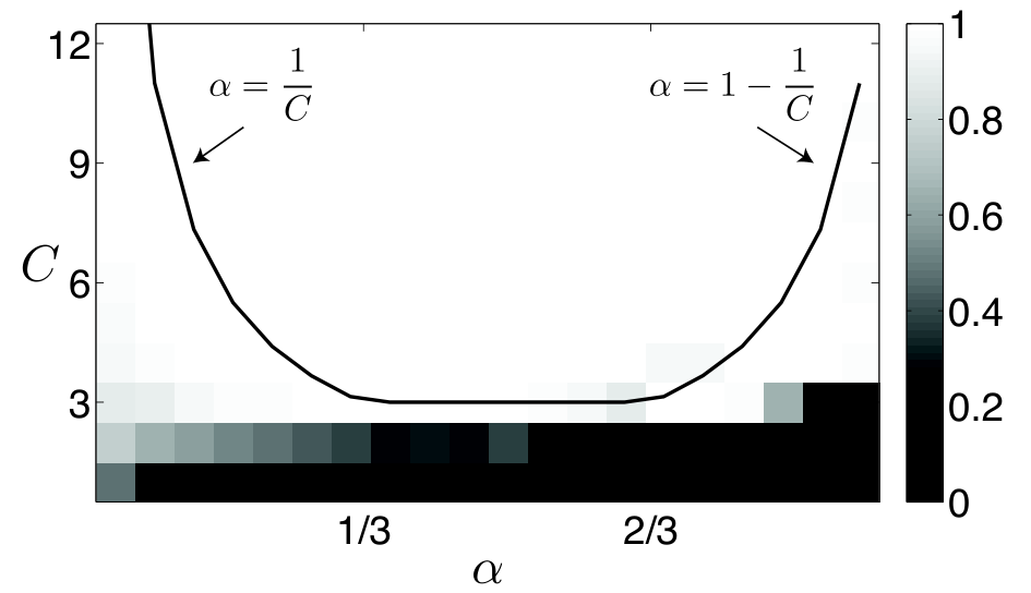
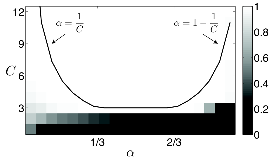
Experiment 1: We fix the signal size to $N=2^{22}$ and run the algorithm $1000$ times to estimate the success probability for $\alpha\in(0,\frac{1}{3}]$ and $1\leq C\leq 12$ . The hashing scheme used is as described in Section VII-D. Fig. 7 shows the simulation result. Albeit the asymptotic behavior of the error probability is only guaranteed for $C=(\frac{1}{\alpha}\vee\frac{1}{1-\alpha})$ , we observe much better results in practice. Indeed, $C=4$ already gives a probability of success very close to one over a large range of $\alpha$ , and only up to $C=6$ seems to be required for the largest values of $\alpha$ .
•

Experiment 2: We repeat here experiment 1, but instead of deterministic hashing matrices, we now pick $\Sigma_{i}$ , $i\in[C]$ , uniformly at random from $\operatorname{GL}(n,\mathbb{F}_{2})$ . The result is shown in Fig. 8. We observer that this scheme performs at least as well as the deterministic one.
•

Experiment 3: In this experiment, we investigate the sensitivity of the algorithm to the value of the parameter $\beta=K/B$ ; the average number of non-zero coefficients per bin. As we explained, in our hash design we use $\beta\approx 1$ . However, using larger values of $\beta$ is appealing from a computational complexity point of view. For the simulation, we fix $N=2^{22}$ , $B=2^{17}$ , $C=4$ , and vary $\alpha$ between $0.7$ and $0.9$ , thus changing $K$ and as a result $\beta$ . Fig. 9 show the simulation results. For $\beta\approx 0.324$ , the algorithm succeeds with probability very close to one. Moreover, for values of $\beta$ larger than $3$ , success probability sharply goes to $0$ .

•

Runtime measurement: We compare the runtime of the SparseFHT algorithm with a straightforward implementation of the fast Hadamard transform. The result is shown in Fig. 10 for $N=2^{15}$ . SparseFHT performs much faster for $0<\alpha<2/3$ .

It is also intersting to identify the range of $\alpha$ for which SparseFHT has a lower runtime than the conventional FHT. We define $\alpha^{*}$ , the largest value of $\alpha$ such that SparseFHT is faster than FHT for any lower value of $\alpha$ . That is

\displaystyle\alpha^{*}=\sup_{\alpha\in(0,1)}\{\alpha\,:\,\forall\alpha^{\prime}\leq\alpha,\ T_{FHT}(n)>T_{SFHT}(\alpha^{\prime},n)\},

where $T_{FHT}$ and $T_{SFHT}$ are the runtimes of the conventional FHT and SparseFHT, respectively. We plot $\alpha^{*}$ as a function of $n=\log_{2}N$ in Fig. 11.

Fig. 10: Comparison of the Median runtime in ms of the SparseFHT and conventional FHT for

N=2^{15}

and for different values of

\alpha

. Confidence interval where found to be negligible and are omitted here. Lower runtime is better.

Fig. 11: In this figure, we plot

n=\log_{2}N

against

\alpha^{*}

, the largest value of

\alpha

such that SparseFHT runs faster than the conventional FHT for all values of

\alpha

smaller or equal. When FHT is always faster, we simply set

\alpha^{*}=0

. Larger values are better.

Remark 9.

In the computation of the complexity in Section V-B, we have assumed that matrix-vector multiplications in $\mathbb{F}_{2}^{n}$ can be done in $O(1)$ . In general, it is not true. However, the deterministic hashing scheme of the algorithm is nothing but a circular bit shift that can be implemented in a constant number of operations, independent of the vector size $n$ .

If one is given $\Sigma$ , some matrix from $\mathbb{F}_{2}^{n\times n}$ , and its inverse transpose $\Sigma^{-T}$ , the overall complexity of the algorithm would nonetheless be unchanged. First, we observe that it is possible to compute the inner product of two vectors in constant time using bitwise operations and a small look-up table¹¹ 1 http://graphics.stanford.edu/~seander/bithacks.html#ParityLookupTable. Now, given the structure of $\Psi_{b}$ , computing $\Sigma\Psi_{b}m$ in Algorithm 1 only requires $\log_{2}K$ inner products. Thus the complexity of Algorithm 1 is unchanged. Finally, (7) can be split into pre-computing $\Sigma^{-T}\Psi_{b}k$ at the same time as we subsample the signal (in $O(\log_{2}K)$ ), and computing the inner product between $\hat{v}$ and the $n-b$ first columns of $\Sigma$ when doing the decoding ( $O(\log_{2}\frac{N}{K})$ ).

IX Conclusion

We presented a new algorithm to compute the Hadamard transform of a signal of length $N$ which is $K$ -sparse in the Hadamard domain. The algorithm presented has complexity $O(K\log_{2}K\log_{2}\frac{N}{K})$ and only requires $O(K\log_{2}\frac{N}{K})$ time-domain samples. We show that the algorithm correctly reconstructs the Hadamard transform of the signal with high probability asymptotically going to one.

The performance of the algorithm is also evaluated empirically through simulation, and its speed is compared to that of the conventional fast Hadamard transform. We find that considerable speed-up can be obtained, even for moderate signal length (e.g. $N=2^{10}$ ) with reasonnable sparsity assumptions.

However, from the statement of Proposition 2, it will be apparent to the reader that the algorithm is absolutely not robust to noise. In fact, at very large signal size, the machine noise, using double-precision floating point arithmetic, proved to be problematic in the simulation. To make the algorithm fully practical, a robust estimator is needed to replace Proposition 2, and is, so far, left for future work.

References

[1] W. Pratt, J. Kane, and H. C. Andrews, “Hadamard transform image coding,” in Proceedings of the IEEE, 1969, pp. 58–68.
[2] 3GPP TS 25.213 V11.4.0 Release 11, “Spreading and modulation (fdd),” 2013.
[3] K. J. Horadam, Hadamard Matrices and Their Applications. Princeton University Press, 2007.
[4] S. Haghighatshoar and E. Abbe, “Polarization of the Rényi information dimension for single and multi terminal analog compression,” arXiv preprint arXiv:1301.6388, 2013.
[5] A. Hedayat and W. Wallis, “Hadamard matrices and their applications,” The Annals of Statistics, pp. 1184–1238, 1978.
[6] M. H. Lee and M. Kaveh, “Fast Hadamard transform based on a simple matrix factorization,” Acoustics, Speech and Signal Processing, IEEE Transactions on, vol. 34, no. 6, pp. 1666–1667, 1986.
[7] J. R. Johnson and M. Pueschel, “In search of the optimal Walsh-Hadamard transform,” in Acoustics, Speech, and Signal Processing, 2000. ICASSP ’00. Proceedings. 2000 IEEE International Conference on, 2000, pp. 3347–3350.
[8] A. C. Gilbert, S. Guha, P. Indyk, S. Muthukrishnan, and M. Strauss, “Near-optimal sparse fourier representations via sampling,” in Proceedings of the thiry-fourth annual ACM symposium on Theory of computing. ACM, 2002, pp. 152–161.
[9] A. C. Gilbert, M. J. Strauss, and J. A. Tropp, “A Tutorial on Fast Fourier Sampling,” Signal Processing Magazine, IEEE, vol. 25, no. 2, pp. 57–66, 2008.
[10] D. Lawlor, Y. Wang, and A. Christlieb, “Adaptive sub-linear Fourier algorithms,” arXiv.org, Jul. 2012.
[11] H. Hassanieh, P. Indyk, D. Katabi, and E. Price, “Simple and practical algorithm for sparse Fourier transform,” Proceedings of the Twenty-Third Annual ACM-SIAM Symposium on Discrete Algorithms, pp. 1183–1194, 2012.
[12] ——, “Nearly optimal sparse Fourier transform,” Proceedings of the 44th symposium on Theory of Computing, pp. 563–578, 2012.
[13] B. Ghazi, H. Hassanieh, P. Indyk, D. Katabi, E. Price, and L. Shi, “Sample-Optimal Average-Case Sparse Fourier Transform in Two Dimensions,” arXiv.org, Mar. 2013.
[14] S. Pawar and K. Ramchandran, “A hybrid DFT-LDPC framework for fast, efficient and robust compressive sensing,” in Communication, Control, and Computing (Allerton), 2012 50th Annual Allerton Conference on, 2012, pp. 1943–1950.
[15] ——, “Computing a k-sparse n-length Discrete Fourier Transform using at most 4k samples and O(k log k) complexity,” arXiv.org, May 2013.
[16] T. Richardson and R. L. Urbanke, Modern coding theory. Cambridge University Press, 2008.
[17] N. C. Wormald, “Differential Equations for Random Processes and Random Graphs,” The Annals of Applied Probability, vol. 5, no. 4, pp. 1217–1235, Nov. 1995.
[18] M. G. Luby, M. Mitzenmacher, M. A. Shokrollahi, and D. A. Spielman, “Efficient erasure correcting codes,” Information Theory, IEEE Transactions on, vol. 47, no. 2, pp. 569–584, 2001.

Appendix A Proof of the Properties of the WHT

A-A Proof of Property 1

\sum_{m\in\mathbb{F}_{2}^{n}}(-1)^{\left\langle k\,,\,m\right\rangle}x_{m+p}=\sum_{m\in\mathbb{F}_{2}^{n}}(-1)^{\left\langle k\,,\,m+p\right\rangle}x_{m}.

And the proof follows by taking $(-1)^{\left\langle k\,,\,p\right\rangle}$ out of the sum and recognizing the Hadamard transform of $x_{m}$ . $\blacksquare$

A-B Proof of Property 2

As we explained, it is possible to assign an $N\times N$ matrix $\Pi$ to the permutation $\pi$ as follows

(\Pi)_{i,j}=\begin{cases}1&\text{if $j=\pi(i)\Leftrightarrow i=\pi^{-1}(j)$}\\ 0&\text{otherwise.}\end{cases}.

Let $\pi_{1}$ and $\pi_{2}$ be the permutations associated with $\Pi_{1}$ and $\Pi_{2}$ . Since $(H_{N})_{i,j}=(-1)^{\left\langle i\,,\,j\right\rangle}$ , the identity (1) implies that

(-1)^{\left\langle\pi_{2}(i)\,,\,j\right\rangle}=(-1)^{\left\langle i\,,\,\pi_{1}^{-1}(j)\right\rangle}.

Therefore, for any $i,j\in\mathbb{F}_{2}^{n}$ , $\pi_{1},\pi_{2}$ must satisfy $\left\langle\pi_{2}(i)\,,\,j\right\rangle=\left\langle i\,,\,\pi_{1}^{-1}(j)\right\rangle$ . By linearity of the inner product, one obtains that

$\displaystyle\left\langle\pi_{2}(i+k)\,,\,j\right\rangle$	$\displaystyle=$	$\displaystyle\left\langle i+k\,,\,\pi_{1}^{-1}(j)\right\rangle$
	$\displaystyle=$	$\displaystyle\left\langle i\,,\,\pi_{1}^{-1}(j)\right\rangle+\left\langle k\,,\,\pi_{1}^{-1}(j)\right\rangle$
	$\displaystyle=$	$\displaystyle\left\langle\pi_{2}(i)\,,\,j\right\rangle+\left\langle\pi_{2}(k)\,,\,j\right\rangle.$

As $i,j\in\mathbb{F}_{2}^{n}$ are arbitrary, this implies that $\pi_{2}$ , and by symmetry $\pi_{1}$ , are both linear operators. Hence, all the permutations satisfying (1) are in one-to-one correspondence with the elements of $\operatorname{GL}(n,\mathbb{F}_{2})$ . $\blacksquare$

A-C Proof of Property 3

Since $\Sigma$ is non-singular, then $\Sigma^{-1}$ exists. It follows from the definition of the WHT that

	$\displaystyle\sum_{m\in\mathbb{F}_{2}^{n}}(-1)^{\left\langle k\,,\,m\right\rangle}x_{\Sigma m}$	$\displaystyle=\sum_{m\in\mathbb{F}_{2}^{n}}(-1)^{\left\langle k\,,\,\Sigma^{-1}m\right\rangle}x_{m}$
		$\displaystyle=\sum_{m\in\mathbb{F}_{2}^{n}}(-1)^{\left\langle\Sigma^{-T}k\,,\,m\right\rangle}x_{m}.$

This completes the proof. $\blacksquare$

A-D Proof of Property 4

\sum_{m\in\mathbb{F}_{2}^{b}}(-1)^{\left\langle k\,,\,m\right\rangle}x_{\Psi_{b}m}\\ \hfill\begin{array}[]{cl}=&\frac{1}{\sqrt{N}}\sum\limits_{m\in\mathbb{F}_{2}^{b}}(-1)^{\left\langle k\,,\,m\right\rangle}\sum\limits_{p\in\mathbb{F}_{2}^{n}}(-1)^{\left\langle\Psi_{b}m\,,\,p\right\rangle}X_{p}\\ =&\frac{1}{\sqrt{N}}\sum\limits_{p\in\mathbb{F}_{2}^{n}}X_{p}\sum\limits_{m\in\mathbb{F}_{2}^{b}}(-1)^{\left\langle m\,,\,k+\Psi_{b}^{T}p\right\rangle}.\end{array}

(9)

In the last expression, if $p=\Psi_{b}k+i$ with $i\in\mathcal{N}(\Psi_{b}^{T})$ then it is easy to check that the inner sum is equal to $B$ , otherwise it is equal to zero. Thus, by proper renormalization of the sums one obtains the proof. $\blacksquare$

Appendix B Proof of Proposition 2

We first show that if multiple coefficients fall in the same bin, it is very unlikely that 1) is fulfilled. Let $\mathcal{I}_{k}=\{j\,|\mathcal{H}j=k\}$ be the set of variable indices hashed to bin $k$ . This set is finite and its element can be enumerated as $\mathcal{I}_{k}=\{j_{1},\ldots,j_{\frac{N}{B}}\}$ . We show that a set $\{X_{j}\}_{j\in\mathcal{I}_{k}}$ is very unlikely, unless it contains only one non-zero element. Without loss of generality, we consider $\sum_{j\in\mathcal{I}_{k}}X_{j}=1$ . Such $\{X_{j}\}_{j\in\mathcal{I}_{k}}$ is a solution of

\begin{bmatrix}1&\cdots&1\\ (-1)^{\left\langle\sigma_{1}\,,\,j_{1}\right\rangle}&\cdots&(-1)^{\left\langle\sigma_{1}\,,\,j_{\frac{N}{B}}\right\rangle}\\ \vdots&\ddots&\vdots\\ (-1)^{\left\langle\sigma_{n-b}\,,\,j_{1}\right\rangle}&\cdots&(-1)^{\left\langle\sigma_{n-b}\,,\,j_{\frac{N}{B}}\right\rangle}\end{bmatrix}\begin{bmatrix}X_{j_{1}}\\ \vdots\\ X_{j_{\frac{N}{B}}}\end{bmatrix}=\begin{bmatrix}1\\ \pm 1\\ \vdots\\ \pm 1\end{bmatrix},

where $\sigma_{i},i\in\{1,\ldots,n\}$ denotes the $i$ -th column of the matrix $\Sigma$ . The left hand side matrix in the expression above, is $(n-b+1)\times 2^{n-b}$ . As $\sigma_{1},\ldots,\sigma_{n-b}$ form a basis for $\mathcal{I}_{k}$ , all the columns are different and are (omitting the top row) the exhaustive list of all $2^{n-b}$ possible $\pm 1$ vectors. Thus the right vector is always one of the columns of the matrix and there is a solution with only one non-zero component ( $1$ -sparse solution) to this system whose support can be uniquely identified. Adding any vector from the null space of the matrix to this initial solution yields another solution. However, as we will show, due to its structure this matrix is full rank and thus its null space has dimension $2^{n-b}-n+b-1$ . Assuming a continuous distribution on the non-zero components $X_{i}$ , the probability that $\{X_{i}\}_{i\in\mathcal{I}_{k}}$ falls in this null space is zero.

To prove that the matrix is indeed full rank, let us first focus on the rank of the sub-matrix obtained by removing the first row. This submatrix itself always contains $M=-2I+\mathds{1}\mathds{1}^{T}$ , where $I$ is the identity matrix of order $n-b$ and $\mathds{1}$ is the all-one vector of dimension $(n-b)$ . One can simply check that $M$ is a symmetric matrix, thus by spectral decomposition, it has $n-b$ orthogonal eigen-vectors $v_{i},i\in[n-b]$ . It is also easy to see that the normalized all-one vector $v_{0}=\frac{\mathds{1}}{\sqrt{n-b}}$ of dimension $n-b$ is an eigen-vector of $M$ with eigen-value $\lambda_{0}=n-b-2$ . Moreover, assuming the orthonormality of the eigen-vectors, it results that $v_{i}^{T}Mv_{i}=\lambda_{i}=-2$ , where we used $v_{i}^{T}\mathds{1}=v_{i}^{T}v_{0}=0$ for $i\neq 0$ . Thus, for $n-b\neq 2$ all of the eigen-vlaues are non-zero and $M$ is invertible, which implies that the sub-matrix resulted after removing the first row is full rank. In the case where $n-b=2$ , one can notice that the Hadamard matrix of size 2 will be contained as a submatrix, and thus the matrix will be full rank.

Now it remains to prove that initial matrix is also full rank with a rank of $n-b+1$ . Assume that the columns of the matrix are arranged in the lexicographical order such that neglecting the first row, the first and the last column are all $1$ and all $-1$ . If we consider any linear combination of the rows except the first one, it is easy to see that the first and the last element in the resulting row vector have identical magnitudes but opposite signs. This implies that the all-one row cannot be written as a linear combination of the other rows of the matrix. Therefore, the rank of the matrix must be $n-b+1$ .

To prove (7), let $\Sigma_{L}$ and $\Sigma_{R}$ be the matrices containing respectively the first $n-b$ and the last $b$ columns of $\Sigma$ , such that $\Sigma=[\Sigma_{L}\,\Sigma_{R}]$ . If there is only one coefficient in the bin, then (6) implies that $\hat{v}=[\,(j^{T}\Sigma_{L})\ 0\,]^{T}$ . Using definitions (2) and (5), we obtain that $\Psi_{b}\mathcal{H}j=[\,0\ (j^{T}\Sigma_{R})\,]^{T}$ . We observe that they sum to $\Sigma^{T}j$ and the proof follows. $\blacksquare$

Appendix C Proof of Proposition 3

For $t\in[K]$ , let $H_{t}$ denote the size of the random set obtained by picking $t$ objects from $[N]$ independently and uniformly at random with replacement. Let $a_{t}$ and $v_{t}$ denote the average and the variance of $H_{t}$ for $t\in[K]$ . It is easy to see that $\{H_{t}\}_{t\in[K]}$ is a Markov process. Thus, we have

\displaystyle\mathbb{E}\left[H_{t+1}-H_{t}|H_{t}\right]=(1-H_{t}/N),

because the size of the random set increases if an only if we choose an element from $[N]\backslash H_{t}$ . This implies that $a_{t+1}=1+\gamma a_{t}$ , where $\gamma=1-\frac{1}{N}$ . Solving this equation we obtain that

\displaystyle a_{t}=\sum_{r=0}^{t}\gamma^{r}=\frac{1-\gamma^{t+1}}{1-\gamma}=N(1-\gamma^{t+1}).

(10)

In particular, $a_{K}=N(1-(1-\frac{1}{N})^{K})$ , which implies that $\mathbb{E}\left[\frac{H_{K}}{K}\right]=\frac{N}{K}(1-(1-\frac{1}{N})^{K})$ . One can check that for $K=N^{\alpha}$ , $0<\alpha<1$ , as $N$ tends to infinity $\mathbb{E}\left[\frac{H_{K}}{K}\right]$ converges to $1$ . To find the variance of $H_{t}$ , we use the formula

\displaystyle\text{Var}(H_{t+1})=\text{Var}(H_{t+1}|H_{t})+\text{Var}(\mathbb{E}\left[H_{t+1}|H_{t})\right]).

(11)

Therefore, we obtain that

\displaystyle\text{Var}(\mathbb{E}\left[H_{t+1}|H_{t}\right])=\text{Var}(1+\gamma H_{t})=\gamma^{2}v_{t}.

(12)

Moreover, for the first part in (11), we have

$\displaystyle\text{Var}(H_{t+1}\|H_{t})$	$\displaystyle=\mathbb{E}_{H_{t}}\{\text{Var}(H_{t+1}\|H_{t}=h_{t})\}$
	$\displaystyle=\mathbb{E}_{H_{t}}\{\text{Var}(H_{t+1}-H_{t}\|H_{t}=h_{t})\}$
	$\displaystyle\stackrel{{\scriptstyle(I)}}{{=}}\mathbb{E}\left[\frac{H_{t}}{N}\left(1-\frac{H_{t}}{N}\right)\right]$
	$\displaystyle=\frac{a_{t}}{N}+\frac{a_{t}^{2}+v_{t}}{N^{2}},$	(13)

where in $(I)$ we used the fact that given $H_{t}$ , $H_{t+1}-H_{t}$ is a Bernoulli random variable with probability $\frac{H_{t}}{N}$ , thus its variance in equal to $\frac{H_{t}}{N}(1-\frac{H_{t}}{N})$ . Combining (12) and (13), we obtain that

\displaystyle v_{t+1}=\left(\gamma^{2}+\frac{1}{N^{2}}\right)v_{t}+\frac{a_{t}}{N}\left(1+\frac{a_{t}}{N}\right).

(14)

From (10), it is easy to see that $a_{t}$ is increasing in $t$ . Moreover, from (14) it is seen that $v_{t+1}$ is increasing function of $a_{t}$ , thus, if we consider the following recursion

\displaystyle w_{t+1}=\left(\gamma^{2}+\frac{1}{N^{2}}\right)w_{t}+\frac{a_{K}}{N}\left(1+\frac{a_{K}}{N}l\right),

then for any $t\in[K]$ , $v_{t}\leq w_{t}$ . As $w_{t}$ is also an increasing sequence of $t$ , we obtain that

	$\displaystyle v_{K}$	$\displaystyle\leq w_{K}\leq w_{\infty}=\frac{a_{K}}{N}\left(1+\frac{a_{K}}{N}\right)/\left(1-\gamma^{2}-\frac{1}{N^{2}}\right)$
		$\displaystyle=\frac{a_{K}}{2}\left(1+\frac{a_{K}}{N}\right)/\left(1-\frac{1}{N}\right).$

Using Chebyshev’s inequality, we obtain that for any $\epsilon>0$

\displaystyle\mathbb{P}\left\{\frac{H_{K}}{K}\geq(1+\epsilon)\right\}\leq\frac{v_{K}}{K^{2}(\epsilon+1-\frac{a_{K}}{K})^{2}}=\Theta\left(\frac{1}{\epsilon^{2}K}\right).

Obviously, $\frac{H_{K}}{K}\leq 1$ , thus $\frac{H_{K}}{K}$ converges to $1$ in probability as $N$ and as a result $K$ tend to infinity. $\blacksquare$

Appendix D Proof of Proposition 9

Let $S$ be any set of variable nodes of size at most $\eta K$ , where we will choose $\eta$ later. the average degree of variable nodes in $S$ is $C$ . Let $\mathcal{N}_{i}(S),i\in[C]$ be the check neighbors of ${\cal G}$ in hash $i$ . If for at least one of the hashes $i\in[C]$ , $|\mathcal{N}_{i}(S)|>\frac{|S|}{2}$ , it results that there is at least one check node of degree $1$ ( a singleton) among the neighbors, which implies that the peeling decoder can still proceed to decode further variable nodes.

Let ${\cal E}^{i}_{s}$ denote the event that a specific subset $A$ of size $s$ of variable nodes has at most $\frac{s}{2}$ check neighbors in hash $i$ . Also let ${\cal E}_{s}=\cap_{i=1}^{C}{\cal E}^{i}_{s}$ . By the construction of ${\cal G}$ , it is easy to see that $\mathbb{P}\left\{{\cal E}_{s}\right\}=\prod_{i=1}^{C}\mathbb{P}\left\{{\cal E}_{s}^{i}\right\}$ . Let $T$ be any subset of check nodes in hash $i$ of size $\frac{s}{2}$ . The probability that all the neighbors of $A$ in hash $i$ belong to a specific set $T$ of size $\frac{s}{2}$ is equal to $(\frac{s}{2B})^{s}$ . Taking a union bound over ${B\choose s/2}$ of all such sets, it is seen that $\mathbb{P}\left\{{\cal E}_{s}\right\}\leq{B\choose s/2}(\frac{s}{2B})^{s}$ , which implies that $\mathbb{P}\left\{{\cal E}^{i}_{s}\right\}\leq\big({B\choose s/2}(\frac{s}{2B})^{s}\big)^{C}$ . Taking a union bound over all possible subsets of size $s$ of variables, we obtain that

	$\displaystyle\mathbb{P}\left\{F_{s}\right\}$	$\displaystyle\leq{K\choose s}\mathbb{P}\left\{{\cal E}_{s}\right\}\leq{K\choose s}\left({B\choose s/2}\left(\frac{s}{2B}\right)^{s}\right)^{C}$
		$\displaystyle\leq\left(\frac{eK}{s}\right)^{s}\left(\frac{2eB}{s}\right)^{sC/2}\left(\frac{s}{2B}\right)^{sC}\leq\frac{u^{s}s^{s(C/2-1)}}{K^{s(C/2-1)}},$

where $u=e^{C/2+1}(\frac{\beta}{2})^{C/2}$ and where $F_{s}$ denotes the event that the peeling decoder fail to decode a set of variables of size $s$ . We also used the fact that for $n\geq m$ , ${n\choose m}\leq(\frac{n\,e}{m})^{m}$ and $\mathbb{P}\left\{F_{1}\right\}=\mathbb{P}\left\{F_{2}\right\}=0$ . Selecting $\eta=\frac{1}{2u^{2/(C-2)}}$ and applying the union bound, we obtain that

	$\displaystyle\mathbb{P}\left\{F\right\}$	$\displaystyle\leq\sum_{s=1}^{\eta K}\mathbb{P}\left\{F_{s}\right\}=\sum_{s=3}^{\eta K}\mathbb{P}\left\{F_{s}\right\}=\sum_{s=3}^{\eta K}\frac{u^{s}s^{s(C/2-1)}}{K^{s(C/2-1)}}$
		$\displaystyle=O\left(\frac{1}{K^{3(C/2-1)}}\right)+\sum_{s=4}^{\eta K}\left(\frac{1}{2}\right)^{s}=O\left(\frac{1}{K^{3(C/2-1)}}\right),$

where $F$ is the event that the peeling decoder fails to decode all the variables. This completes the proof. $\blacksquare$

A Fast Hadamard Transform for Signals with Sub-linear Sparsity in the Transform Domain

Abstract

Index Terms:

I Introduction

Definition 1.

II Main Results

Theorem 1.

Remark 1.

Remark 2.

III Walsh-Hadamard Transform and its Properties

III-A Basic Properties

Property 1 (Shift/Modulation).

Property 2.

Remark 3.

Property 3 (Permutation).

Remark 4.

Property 4 (Downsampling/Aliasing).

Remark 5.

Remark 6.

IV Hadamard Hashing Algorithm

Proposition 1 (Hashing).

IV-A Properties of Hadamard Hashing

Proposition 2 (Collision detection / Support estimation).

V Sparse Fast Hadamard Transform

V-A Explanation of the Algorithm

V-B Complexity Analysis

VI Performance Analysis of the very Sparse Regime

VI-A Hash Construction

VI-B Random Bipartite Graph Construction

VI-B1 Random Support Model

Proposition 3.

VI-B2 ‘Balls and Bins’ Model 𝒢⁡(K,B,C){\cal G}(K,B,C)

VI-B3 Ensemble of Graphs Generated by Hashing

Proposition 4.

Proof:

Proposition 5.

Proof:

Remark 7.

VI-B4 Edge Degree Distribution Polynomial

Proposition 6.

Proof:

Proposition 7.

Proof:

VI-B5 Average Check Degree Parameter β\beta

VI-C Performance Analysis of the Peeling Decoder

VI-C1 Wormald’s Method

Proposition 8.

Proposition 9.

VI-C2 Analysis based on Belief Propagation over Sparse Graphs

VII Performance Analysis of the Less Sparse Regime

VII-A Hash Construction

VII-B Bipartite Graph Representation

VII-C Performance Analysis of the Peeling Decoder

Definition 2.

Proposition 10.

Proposition 11.

Proof:

Remark 8.

Proposition 12.

Proof:

VII-D Generalized Hash Construction

VIII Experimental Results

Remark 9.

IX Conclusion

References

Appendix A Proof of the Properties of the WHT

A-A Proof of Property 1

A-B Proof of Property 2

A-C Proof of Property 3

A-D Proof of Property 4

Appendix B Proof of Proposition 2

Appendix C Proof of Proposition 3

Appendix D Proof of Proposition 9

VI-B2 ‘Balls and Bins’ Model ${\cal G}(K,B,C)$

VI-B5 Average Check Degree Parameter $\beta$