Potts model, parametric maxflow and $k$-submodular functions

This paper addresses the problem of minimizing an energy function with Potts interaction terms. This energy has found a widespread usage in computer vision after the seminal work of Boykov et al. [4] who proposed an efficient approximation algorithm for this NP-hard problem called alpha expansion.

The algorithm of [4] is based on the maxflow algorithm, also known as graph cuts. Each iteration involves $k$ maxflow computations, where $k$ is the number of labels. Several techniques were proposed for improving the efficiency of these computations. The most relevant to us is the method of Kovtun [19, 20] which computes a part of an optimal solution via $k$ maxflow computations. We can then fix “labeled” nodes and run the alpha expansion algorithm for the remaining nodes. Such scheme was a part of the “Reduce, Reuse, Recycle” approach of Alahari et al. [1].

Our main contribution is to improve the efficiency of Kovtun’s method from $k$ maxflow computations to $\lceil 1+\log_{2}k\rceil$ computations on graphs of equivalent sizes. In some applications the method labels a significant fraction of nodes [19, 20, 1], so our techique gives a substantial speed-up. We may get an improvement even when there are few labeled nodes: it is reported in [1] that using flow from Kovtun’s computations always speeds up the alpha expansion algorithm for unlabeled nodes.

The idea of our approach is to cast the problem as another minimization problem with Tree Metrics, and then generalize the algorithm of Felzenszwalb et al. [7] for Tree Metrics by allowing more general unary terms. This generalization is our second contribution. Finally, we discuss some connections to $k$-submodular functions.

We also mention the “FastPD” method of Komodakis et al. [17, 18]. The default version of FastPD for the Potts energy produces the same answer as the alpha expansion algorithm but faster, since it maintains not only primal variables (current solution) but also dual variables (“messages”). Intuitively, it allows to reuse flow between different maxflow computations. An alternative method for reusing flow was used by Alahari et al. [1], who reported similar speed-ups.

The Potts energy for labeling $x\in{\cal L}^{V}$ is given by

Here $V$ is the set of nodes, $E$ is the set of edges, ${\cal L}$ is the set of labels, $\lambda_{ij}$ are non-negative constants and $[\cdot]$ is the Iverson bracket. It is well-known that computing a minimizer of (1) is NP-hard when $|{\cal L}|\geq 3$ [4].

Let us review the method of Kovtun [19, 20] for obtaining a part of an optimal solution. (The method is applicable to general functions - see [19, 20, 24]; here we consider only the Potts energy, in which case the formulation simplifies considerably.) For a label $a\!\in\!{\cal L}$ denote $\bar{a}\!=\!{\cal L}\!-\!\{a\}$, and let $f_{i}(\bar{a})\!=\!\min\limits_{b\in\bar{a}}f_{i}(b)$. Define function $f^{a}:\{a,\bar{a}\}^{V}\!\rightarrow\!\mathbb{R}$ via

(A remark on notation: we typically use letter $x$ for multi-valued labelings and $y$ for binary labelings).

Kovtun’s approach requires minimizing function $f^{a}$ for all $a\in{\cal L}$. A naive way to do this is to use $k$ maxflow computations on a graph with $|V|$ nodes and $|E|$ edges, where $k=|{\cal L}|$. To reduce this to $O(\log k)$ maxflow computations, we will use the following strategy. First, we will define an auxiliary function $g:{\cal D}^{V}\rightarrow\mathbb{R}$ where ${\cal D}={\cal L}\cup\{{\bf o}\}$, ${\bf o}\notin{\cal D}$. We will then present an efficient algorithm for minimizing $g$, and show that a minimizer $x\in\arg\min\{g(x)\>|\>x\in{\cal D}^{V}\}$ determines a minimizer $y\in\arg\min\{f^{a}(y)\>|\>y\in\{a,\bar{a}\}^{V}\}$ for each $a\in{\cal L}$ in the natural way, i.e. $y_{i}=a$ if $x_{i}=a$ and $y_{i}=\bar{a}$ otherwise. Function $g$ will have the following form:

where $d(\cdot,\cdot)$ is a tree metric with respect to a certain tree $T$:

We define $T$ as the star graph rooted at ${\bf o}$, i.e. ${\cal E}=\{\{a,{\bf o}\}\>|\>a\in{\cal L}\}$. All edges are assigned length 1. The unary functions in (3) are set as follows: $g_{i}({\bf o})=0$ and $g_{i}(a)=f_{i}(a)-f_{i}(\bar{a})$ for $a\in{\cal L}$. Function $g$ in eq. (3) is now completely defined. It can be seen that minimizing $f^{a}$ is equivalent to minimizing $g(y)$ over $y\in\{a,{\bf o}\}^{V}$.

The following observation will be crucial.

More generally, we say that function $g_{i}:{\cal D}\rightarrow\mathbb{R}$ is $T$-convex if for any pair of edges $\{a,b\},\{b,c\}\in{\cal E}$ with $a\neq c$ there holds

Clearly, terms $g_{i}$ contructed above are $T$-convex. We will prove the following result for an arbitrary tree $T$ and function $g$ with $T$-convex unary terms $g_{i}$. (Part (a) will imply that Kovtun’s approach indeed reduces to the minimization of the function $g$ above; part (b) will motivate a divide-and-conquer algorithm for minimizing $g$.)

Note, part (a) and a repeated application of Theorem 1 give that any minimizer $x\in{\cal D}^{V}$ of $g$ is a partially optimal labeling for $f$, i.e. $f$ has a minimizer $x^{\ast}\in{\cal L}^{V}$ such that $x^{\ast}_{i}=x_{i}$ for all $i$ with $x_{i}\neq{\bf o}$.

In the next section we consider the case of an arbitrary tree $T$, and present an efficient algorithm for minimizing function $g$ with $T$-convex unary terms. In section 4 we discuss its specialization to the star graph $T$ with unit edge length, and sketch some implementation details. Then in section 5 we describe a connection to $k$-submodular functions. Section 6 gives experimental results, and section 7 presents conclusions.

We build on the work of Kolen [14] and Felzenszwalb et al. [7]. They considered the case when unary functions $g_{i}(\cdot)$ are given by $g_{i}(x_{i})=\lambda_{i}d(x_{i},c_{i})$ where $\lambda_{i}\geq 0$ and $c_{i}$ is a constant node in ${\cal D}$. [14] showed that such function can be minimized via $|{\cal D}|$ maximum flow computations on graphs with $O(|V|)$ nodes and $O(|E|)$ edges. Using a divide-and-conquer approach, [7] improved this to $O(\log|{\cal D}|)$ maxflow computations (plus $O(|{\cal D}|\log|{\cal D}|)$ time for bookkeeping). Their algorithm can be viewed as a generalization of the algorithm in [11, 5, 6] for minimizing Total Variation functionals $g(x)=\sum_{i}g_{i}(x_{i})+\sum_{\{i,j\}}\lambda_{ij}|x_{j}-x_{i}|$ with convex terms $g_{i}$ over $x\in\{1,2,\ldots,k\}^{V}$ (this corresponds to the case when $T$ is a chain with unit lengths).

In this section we show that with an appropriate modification the algorithm of [7] can be applied to function (3) with $T$-convex unary terms, and present a self-contained proof of correctness.¹¹ 1 The proof in [7] relied on results in [14], and used a different argument. In our view, the new proof shows more clearly why the extension to $T$-convex unary terms is possible.

The main step of the algorithm is computing a minimizer $y\in\arg\min\{g(y)\>|\>y\in\{a,b\}^{V}\}$ for some edge $\{a,b\}\in{\cal E}$ (this can be done via a maxflow algorithm). By Theorem 4(b), $y$ gives some information about a minimizer of $g$. This information allows to split the problem into two independent subproblems which can then be solved recursively. We arrive at the following algorithm.

Note that function $g^{c}$ in line 7 is defined on the subgraph of $(V,E)$ induced by $V_{c}$. Indeed, for each edge $\{i,j\}\in E$ with $i\in V_{c}$, $j\in V-V_{c}$ pairwise term $\lambda_{ij}d(x_{i},x_{j})$ is transformed to a unary term $\lambda_{ij}d(x_{i},c)$. It can be checked that this unary term is $T_{c}$-convex.

The following theorem implies that the algorithm is correct; its proof is given in section 3.1.

The algorithm leaves some freedom in line 2, namely the choice of edge $\{a,b\}\in{\cal E}$. Ideally, we would like to choose an edge that splits the tree into approximately equals parts ($|{\cal D}_{a}|\approx|{\cal D}_{b}|$). Unfortunately, this is not always possible; if, for example, $T$ is a star graph then every split will be very unbalanced. To deal with this issue, [7] proposed to expand tree $T$ (and modify the input function accordingly) so that the new tree $T^{\prime}$ admits a more balanced split. Details are given below.

Let $a$ be a node in ${\cal D}$ with two or more neighbors. Let us split these neighbors into non-empty disjoint sets ${\cal N}$, ${\cal N}^{\prime}$ and modify tree $T$ as described in Fig. 2. (This step is inserted before line 2; the new edge $\{a,b\}$ becomes the output of line 2.) We denote ${\cal D}^{\prime}={\cal D}\cup\{b\}$; also, let ${\cal D}^{\prime}_{a}$, ${\cal D}^{\prime}_{b}$ be the connected components of $T^{\prime}$ after removing edge $\{a,b\}$ (with $a\in{\cal D}^{\prime}_{a}$, $b\in{\cal D}^{\prime}_{b}$).

The length of new edge $\{a,b\}$ is set to an infinitesimally small constant $\epsilon>0$. The new unary function $g^{\epsilon}_{i}:{\cal D}^{\prime}\rightarrow\mathbb{R}$ for node $i\in V$ is defined via

where we assume that $g_{i}(b)=g_{i}(a)$, and $u_{i}\in\mathbb{R}$ is chosen in such a way that function $g^{\epsilon}_{i}$ is $T^{\prime}$-convex. (Such $u_{i}$ always exists - see below). The new functional is thus $g^{\epsilon}(x)=\sum_{i\in V}g^{\epsilon}_{i}(x_{i})+\sum_{\{i,j\}\in E}\lambda_{ij}d^{\epsilon}(x_{i},x_{j})$ for $x\in({\cal D}^{\prime})^{V}$, where $d^{\epsilon}$ is the new tree metric.

There holds $|g^{\epsilon}(x)-g(x^{b\mapsto a})|\leq const\cdot\epsilon$ for any $x\in({\cal D}^{\prime})^{V}$, where $x^{b\mapsto a}$ is the labeling obtained from $x$ by assigning label $a$ to nodes with label $b$. Therefore, if $\epsilon$ is small enough then the following holds: if $x\in({\cal D}^{\prime})^{V}$ is an optimal solution of the modified problem then $x^{b\mapsto a}$ is an optimal solution of the original problem.

The cost function used in line 3 can be written as $g^{\epsilon}(y)=const+\epsilon\cdot g^{\prime}(y)$ for all $y\in\{a,b\}^{V}$, where function $g^{\prime}:\{a,b\}^{V}\rightarrow\mathbb{R}$ is defined via

Therefore, minimizing $g^{\epsilon}$ over $\{a,b\}^{V}$ is equivalent to minimizing $g^{\prime}$ (and thus the minimizer does not depend on $\epsilon$).

To summarize, we showed that the SPLIT algorithm remains correct if we replace line 2 with the tree modification step described above, and in line 3 compute $y\in\arg\min\{g^{\prime}(y)\>|\>y\in\{a,b\}^{V}\}$. Also, in line 10 we need to convert labeling $x^{b}$ to $(x^{b})^{b\mapsto a}$ before merging with $x^{a}$.

In this section we sketch implementation details of Algorithm 1 applied to the function constructed in section 2 (so $T$ is a star graph with nodes ${\cal D}={\cal L}\cup\{{\bf o}\}$). We will discuss, in particular, how to extract optimal flows.

We use the edge insertion operation at each call of SPLIT except when ${\cal D}=\{a,{\bf o}\}$ for some $a\in{\cal L}$. Thus, computations can be described in terms of a binary tree whose nodes correspond to subsets of labels ${\cal A}\subseteq{\cal L}$ (Fig. 3). Let $\Omega$ be the set of nodes of this tree. For each ${\cal A}\in\Omega$ we run a maxflow algorithm; let $V_{\cal A}\subseteq V$ be the set of nodes involved in this computation. Note that sets $V_{\cal A}$ for nodes ${\cal A}$ at a fixed depth form a disjoint union of $V$ (except possibly the last level). Therefore, these maxflow computations can be treated as a single maxflow on the graph of the original size. The total number of such computations is $\lceil 1+\log_{2}k\rceil$ (the number of levels of the tree).

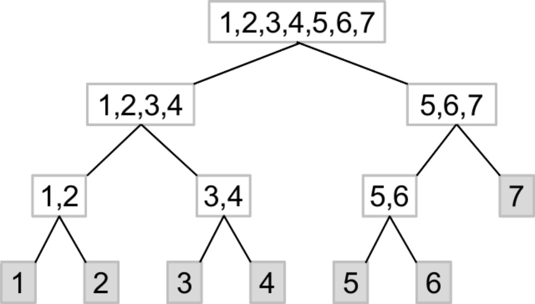For each ${\cal A}\in\Omega$ we set up a graph with the set of nodes $V_{\cal A}\cup\{s,t\}$ and the cut function

($S\stackrel{{\scriptstyle.}}{{\cup}}T=V_{\cal A}$). To define $u^{\cal A}_{i}$, we need to specify the meaning of the source $s$ and the sink $t$. For non-leaf nodes ${\cal A}\in\Omega$ the source corresponds to the left child ${\cal A}_{\ell}$ and the sink corresponds to the right child ${\cal A}_{r}$; we then have

where we use the current value of $g_{i}({\bf o})$ (it is zero initially and then gets decreased). For a leaf ${\cal A}=\{a\}$ we use a different intepretation: $s$ corresponds to label $a$ and $t$ corresponds to label ${\bf o}$, therefore $u^{\cal A}_{i}=g_{i}({\bf o})-g_{i}(a)$.

We perform all maxflow computations on a single graph. We use the Boykov-Kolmogorov algorithm [3] with flow and search trees recycling [13]. We maintain values $u_{i}$ for nodes $i\in V$ that give the current cut functions encoded by the residual graph. After computing maxflow at a non-leaf node ${\cal A}$ the residual graph is modified as follows. First, for each arc $(i\rightarrow j)$ from the source to the sink component we do the following:

• 1.

  Set $u_{i}:=u_{i}-\lambda_{ij}$ and $u_{j}:=u_{j}+\lambda_{ij}$; this simulates pushing flow $\lambda_{ij}$ along the path $t\rightarrow j\rightarrow i\rightarrow s$.

• 2.

  Remove arcs $(i\rightarrow j),(j\rightarrow i)$ from the graph.

• 3.

  Update $g_{i}({\bf o}):=g_{i}({\bf o})-\lambda_{ij}$.

Now we need to set unary costs for maxflow computations at the children ${\cal A}_{\ell}$, ${\cal A}_{r}$ of ${\cal A}$. Consider node $i\in V_{{\cal A}_{c}}$, $c\in\{\ell,r\}$. First, we compute the appropriate value $u^{{\cal A}_{c}}_{i}$; if ${\cal A}_{c}$ is not a leaf then we compute interval (9) for ${\cal A}_{c}$ and choose the value $u^{{\cal A}_{c}}_{i}$ from the interval closest to $u_{i}$.²² 2 It can be shown that we only need to know $a^{\ast}\in\arg\min_{a\in{\cal L}}g_{i}(a)$, $g_{i}(a^{\ast})$ and $g_{i}({\bf o})$ for that. Then we change the graph by adding $\delta^{{\cal A}_{c}}_{i}=u^{{\cal A}_{c}}_{i}-u_{i}$ to the capacity of $(s\rightarrow i)$ (or subtracting from the capacity of $(i\rightarrow t)$), and update $u_{i}:=u^{{\cal A}_{c}}_{i}$.

Such monotonicity implies that computations at non-leaf nodes fall into the framework of parametric maxflow of Gallo et al. [8]. As shown in [8], all computations can be done with the same worst-case complexity as a single maxflow computation. However, this requires a more complex implementation, namely running in parallel two push-relabel algorithms. Experiments in [2] suggest that this is less efficient than a naive scheme.

It suffices to specify the flow $\xi_{ij}$ for each arc $(i\rightarrow j)$ with $\{i,j\}\in E$ (the flow from the source and to the sink can then be easily computed). We used the following rule. For each edge we store flow $\xi^{\prime\prime}_{ij}$ after the final maxflow and flow $\xi^{\prime}_{ij}$ immediately before maxflows at the leaves. For each node $i\in V$ we also store leaf ${\cal A}_{i}\in\Omega$ at which node $i$ ended up. We now set flow $\xi_{ij}$ as follows:

• $\bullet$

  if ${\cal A}_{i}={\cal A}_{j}=\{a\}$ set $\xi_{ij}:=\xi^{\prime\prime}_{ij}$

• $\bullet$

  otherwise let ${\cal A}\in\Omega$ be the least common ancestor of ${\cal A}_{i},{\cal A}_{j},\{a\}$ in the binary tree. If $\{a\}$ belongs to the left subtree of ${\cal A}$ then set $\xi_{ij}:=\xi^{\prime}_{ij}$, otherwise set $\xi_{ij}:=\xi^{\prime}_{ji}$.

We hope to prove to correctness of this procedure in a future publication; at the moment we state it as a conjecture that was verified experimentally. We mention that we were not able to find a scheme that would store only one flow per arc.

In this section we discuss some connections between techniques described earlier and $k$-submodular functions introduced in [15, 12]. We also define $k$-submodular relaxations of discrete functions $f:{\cal L}^{V}\rightarrow\mathbb{R}$ which generalize bisubmodular relaxations [16] of pseudo-Boolean functions in a natural way.

References

- [1] K. Alahari, P. Kohli, and P. H. S. Torr. Dynamic hybrid algorithms for MAP inference in discrete MRFs. PAMI, 32(10):1846–1857, 2010.
- [2] M. Babenko, J. Derryberry, A. Goldberg, R. Tarjan, and Y. Zhou. Experimental evaluation of parametric max-flow algorithms. In 6th Int’l conference on Experimental Algorithms (WEA), pages 256–269, 2007.
- [3] Y. Boykov and V. Kolmogorov. An experimental comparison of min-cut/max-flow algorithms for energy minimization in vision. PAMI, 26(9), September 2004.
- [4] Y. Boykov, O. Veksler, and R. Zabih. Fast approximate energy minimization via graph cuts. PAMI, 23(11), 2001.
- [5] A. Chambolle. Total variation minimization and a class of binary MRF models. In EMMCVPR, pages 136–152, November 2005.
- [6] J. Darbon and M. Sigelle. Image restoration with discrete constrained total variation part I: Fast and exact optimization. J. of Math. Imaging and Vision, 26(3):261–276, 2006.
- [7] P. Felzenszwalb, G. Pap, E. Tardos, and R. Zabih. Globally optimal pixel labeling algorithms for tree metrics. In CVPR, 2010.
- [8] G. Gallo, M. D. Grigoriadis, and R. E. Tarjan. A fast parametric maximum flow algorithm and applications. SIAM J. Computing, 18:30–55, 1989.
- [9] P. L. Hammer, P. Hansen, and B. Simeone. Roof duality, complementation and persistency in quadratic 0-1 optimization. Math. Programming, 28:121–155, 1984.
- [10] H. Hirschmüller. Evaluation of cost functions for stereo matching. In CVPR, 2007.
- [11] D. S. Hochbaum. An efficient algorithm for image segmentation, Markov Random Fields and related problems. J. ACM, 48:2:686–701, July 2001.
- [12] A. Huber and V. Kolmogorov. Towards minimizing -submodular functions. In International Symposium on Combinatorial Optimization (ISCO), Apr. 2012.
- [13] P. Kohli and P. H. S. Torr. Efficiently solving dynamic Markov random fields using graph cuts. In ICCV, 2005.
- [14] A. J. W. Kolen. Tree Network and Planar Rectilinear Location Theory. volume 25 of CWI Tracts. CWI, 1986.
- [15] V. Kolmogorov. Submodularity on a tree: Unifying L♮-convex and bisubmodular functions. In 36th Int’l Symposium on Math. Foundations of Comp. Science, Aug. 2011.
- [16] V. Kolmogorov. Generalized roof duality and bisubmodular functions. Discrete Applied Mathematics, 160(4-5):416–426, March 2012.
- [17] N. Komodakis and G. Tziritas. Approximate labeling via graph cuts based on linear programming. PAMI, 29(8):1436–1453, 2007.
- [18] N. Komodakis, G. Tziritas, and N. Paragios. Performance vs computational efficiency for optimizing single and dynamic MRFs: Setting the state of the art with primal-dual strategies. CVIU, 112(1):14 – 29, 2008.
- [19] I. Kovtun. Partial optimal labeling search for a NP-hard subclass of (max,+) problems. In DAGM, pages 402–409, 2003.
- [20] I. V. Kovtun. Image segmentation based on sufficient conditions of optimality in NP-complete classes of structural labelling problems. PhD thesis, IRTC ITS National Academy of Sciences, Ukraine, 2004. (In Ukranian).
- [21] D. Scharstein and R. Szeliski. A taxonomy and evaluation of dense two-frame stereo correspondence algorithms. IJCV, 47(1-3):7–42, Apr. 2002.
- [22] D. Scharstein and R. Szeliski. High-accuracy stereo depth maps using structured light. In CVPR, pages 195–202, 2003.
- [23] A. Shekhovtsov. Efficient graph-based energy minimization methods in computer vision. PhD thesis, Czech Technical University, CMP, Prague, 2013.
- [24] A. Shekhovtsov and V. Hlavac. On partial opimality by auxiliary submodular problems. Control Systems and Computers, 2:71–78, 2012.
- [25] J. Thapper and S. Živný. The power of linear programming for valued CSPs. In FOCS, 2012.
- [26] T. Werner. A linear programming approach to max-sum problem: A review. PAMI, 29(7):1165–1179, 2007.
- [27] B. A. Zalesky. Network flow optimization for restoration of images. J. Appl. Math., 2(4):199–218, 2002.