On the symmetric doubly stochastic matrices that are determined by their spectra
Abstract
A symmetric doubly stochastic matrix is said to be determined by its spectra if the only symmetric doubly stochastic matrices that are similar to are of the form for some permutation matrix The problem of characterizing such matrices is considered here. An “almost” the same but a more difficult problem was proposed by [ M. Fang, A note on the inverse eigenvalue problem for symmetric doubly stochastic matrices, Lin. Alg. Appl., 432 (2010) 2925-2927] as follows: “Characterize all the -tuples such that up to a permutation similarity, there exists a unique symmetric doubly stochastic matrix with spectrum ” In this short note, some general results concerning our two problems are first obtained. Then, we completely solve these two problems for the case Some connections with spectral graph theory are then studied. Finally, concerning the general case, two open questions are posed and a conjecture is introduced.
Keywords:
Doubly stochastic matrices , Inverse eigenvalue problem, Spectral characterizationMSC
15A12, 15A18, 15A51, 05C501 Introduction
An real matrix having each row and column sum equal to 1 is called doubly quasi-stochastic. If, in addition, is nonnegative then is said to be doubly stochastic. The set of all doubly-stochastic matrices is denoted by and the set of all the symmetric elements in will be denoted by For denote by to be the set of all elements of with trace
Three particular elements of are of interest to us. The first is which is the identity matrix and the second which is the matrix whose all entries are The third is which denotes the matrix whose diagonal entries are all zeroes and whose off-diagonal entries are equal to (here for ). In addition, let where denotes the real line. For two matrices (and in particular for row vectors) and the line-segment joining them is denoted by and for any two sets and we write to denote the set of elements in which are not in
Note that it is clear from the definition that an real matrix is doubly quasi-stochastic if and only if and if and only if
The symmetric doubly stochastic inverse eigenvalue problem asks which sets of real numbers occur as the spectrum of an symmetric doubly stochastic matrix. For more information on this problem see, e.g., [7, 8, 9, 10, 13, 14, 15, 16, 17, 18].
Regarding the inverse eigenvalue problem for symmetric doubly stochastic matrices, the following “inaccurate” proposition was presented in [8].
Proposition 1.1
Let be in with If
then there is a positive (i.e. all of its entries are positive) doubly stochastic matrix in such that has spectrum .
In [7] the author presented a counterexample of the preceding proposition as follows.
Theorem 1.2
Let Then there does not exist a symmetric positive doubly stochastic matrix with spectrum
In [4] it was pointed out that the 2-tuple which is the spectrum of is also another counterexample. Moreover, it should be mentioned here that the proof of the preceding theorem (which is the main result of [7]) is done by showing that the matrix has spectrum and the only matrices in that are similar to are of the form for some permutation matrix Based on this, the author suggested the following problem.
Problem 1.3
Characterize all the -tuples with such that up to a permutation similarity, there exists a unique symmetric doubly stochastic matrix with spectrum such is said to characterize permutationally or is said to be permutationally characterized by
Note now that in the language of the preceding problem, the matrix presented above is permutationally characterized by
Two matrices and are said to be permutationally similar if for some permutation matrix Next, we say that a doubly stochastic matrix is determined by its spectra (DS for short) in if for every element of which is similar to then is permutationally similar to If in addition is symmetric then is said to be DS in if is similar to implies that is permutationally similar to For a symmetric doubly stochastic matrix obviously is DS in implies that is DS in However, it is not known whether the converse is true or false and though it is an interesting open problem, it will not be dealt with here. Also, though the problem of characterizing all doubly stochastic matrices that are DS in is very interesting and we will touch on some aspects of this problem, however here we are particularly more interested in the following problem which is very related to Problem 1.3.
Problem 1.4
Characterize all symmetric doubly stochastic matrices that are DS in
All above problems appear to be very difficult and it seems that there is no systematic way under which these problems can be approached (see Section 3). Practically nothing is known about them except perhaps what is mentioned earlier. In addition, we note that if a symmetric doubly stochastic matrix is permutationally characterized by then obviously is DS in So that in order to solve Problem 1.3, we need to solve Problem 1.4 first and then for every solution of this last problem, we have to find the spectrum of
The rest of the paper is organized as follows. Section 2 is mainly concerned with obtaining some general results for our two problems. In Section 3, we completely solve Problem 1.3 and Problem 1.4 for the case which is one of the main results of this paper. In Section 4, we study the close connection of Problem 1.4 with spectral graph theory; more precisely with “regular graphs that are DS.” We conclude in Section 5 by posing two open questions and by introducing a conjecture related to the general case.
2 Some general results
We start our study with the following two lemmas that explore some aspects of the spectral properties of doubly stochastic matrices and are consequences of the Perron-Frobenius theorem (see, e.g. [12]). But first recall that a square nonnegative matrix is irreducible if is not permutationally similar to a matrix of the form where and are square. Otherwise, is said to be reducible.
Lemma 2.1
Every doubly stochastic matrix is permutationally similar to a direct sum of irreducible doubly stochastic matrices.
Lemma 2.2
Let be an irreducible doubly stochastic matrix. If has exactly eigenvalues of unit modulus, then these are the th roots of unity. In addition, if then is a divisor of and is permutationally similar to a matrix of the form
where is doubly stochastic of order for
As a result, we have the following.
Theorem 2.3
Every permutation matrix is DS in
Proof. Suppose first that is an irreducible permutation matrix and let be a doubly stochastic matrix, then clearly is irreducible and all of its eigenvalues are of unit modulus. Therefore by the preceding lemma is a permutation matrix. Now if is reducible then the proof can be completed by using Lemma 2.1.
An immediate consequence is the following corollary.
Corollary 2.4
Let be in where for and such that Then characterizes permutationally a vertex (i.e. symmetric permutation matrix) of
Lemma 2.5
Let be an invertible matrix such that is symmetric doubly stochastic. Then
Proof. Since is symmetric doubly stochastic, then by the spectral theorem for symmetric matrices, there exists an orthogonal matrix whose first column is and the remaining columns are orthogonal to (i.e. the sum of all components in each of the remaining columns is zero) such that where is the zero matrix. Hence But then a simple check shows that and the proof is complete.
Corollary 2.6
The matrices and are DS in
Proof. The first part is obvious, and the second part follows from the preceding lemma. For the third part, we note that and then for any invertible matrix such that is symmetric doubly stochastic we obtain Therefore and where the left-hand side is a nonnegative matrix with row and column sum equals to Thus is symmetric doubly stochastic and then by the preceding lemma, the proof is complete.
Next we need the following auxiliary materials.
Lemma 2.7
The inverse of an invertible doubly quasi-stochastic matrix is doubly quasi-stochastic.
Proof. Multiplying to the left of by we obtain Since is doubly quasi-stochastic, then Similarly, multiplying to the right of by we obtain Thus is doubly quasi-stochastic.
Lemma 2.8
If is an irreducible doubly stochastic matrix such that is doubly stochastic for some invertible matrix , then there exists a doubly stochastic matrix such that
Proof. See [12, Theorem 4.1, p. 123].
Corollary 2.9
The matrices and are DS in
Proof. If is doubly stochastic, then by the preceding lemma, there exists such that Hence The rest of proof can be completed by using a similar argument as that of Corollary 2.6.
It is easy to see that each symmetric doubly stochastic matrix of trace which lies on the line-segment joining to has the property that Also recall that so that is on this line-segment With this in mind, we have the following theorem.
Theorem 2.10
Any point that lies on the line-segment is DS in and hence it is also DS in
Proof. We split the proof into two cases.
- 1.
For then is a convex combination of and From the trace of , we easily obtain so that or Note that is a positive matrix and so it is irreducible. Now if is an invertible matrix such that is doubly stochastic, then by the preceding lemma, there exists a doubly stochastic matrix such that Hence Thus and this shows that is DS in
- 2.
For then is a convex combination of and From the trace of , it is easy to see that in this case and that the proof can be completed in a similar way to that of the previous case.
Knowing that the eigenvalues of are given by then we have the following conclusion.
Corollary 2.11
Let be any point that lies on the line-segment of Then characterizes a unique element of
It should be noted that if two doubly stochastic matrices and are DS in (or ) then their direct sum may not be DS in To see this, it suffices to check that in the matrices and have the same spectrum so that they are similar (as they are symmetric). Moreover, for is an entry of the latter and is not an entry of the first so that they not permutationally similar. However, we have the following.
Theorem 2.12
The matrix is DS in
Proof. If is similar to then obviously the spectrum of is Since is reducible and has the eigenvalue 1 repeated twice, then is permutationally similar to a direct sum of two doubly stochastic matrices and But the traces of and are zeroes so that necessarily the spectrum of and is the same and is equal to By corollary 2.9,
Using a virtually identical proof to that of the preceding theorem, we conclude by mathematical induction the following.
Corollary 2.13
For any positive integers the matrix is DS in
Our next result is concerned with some other doubly stochastic matrices that are DS in For this purpose, we introduce the following notations. In define and then it can be easily checked that so that belongs to the line-segment With this in mind, we conclude with the following result.
Theorem 2.14
Any point on the line-segment is DS in and hence in
Proof. We first prove that and are DS in For, if there exists which is similar to then obviously the spectrum of is By Lemma 2.2, is permutationally similar to a matrix of the form where So that and its eigenvalues are and therefore is similar to By Lemma 2.5, and since rank()=rank()=rank()=1, then and therefore
Now suppose that is similar to then has spectrum and therefore is permutationally similar to but this in turn means that and are permutationally similar. Since then a similar proof to that of Corollary 2.6 shows that is also DS in Finally, using a similar argument to that of Theorem 2.10, the proof can be easily completed.
Recall that two matrices are cospectral if they have the same spectra. We conclude this section by proving that a symmetric doubly stochastic matrix that is DS in may be cospectral to another element of But first, we need the following result for which the proof can be found in [22].
Lemma 2.15
Let where and are square. If then
Theorem 2.16
Let be in and define and let be as defined earlier. Then and are cospectral.
Proof. The characteristic polynomial of is given by By the preceding lemma, i.e. is an eigenvalue of On the other hand, Thus and are cospectral.
3 Particular cases
Recall that Birkhoff’s theorem states that is a convex polytope of dimension where its vertices are the permutation matrices. On the other hand, is a convex polytope of dimension , and its vertices were determined in [11, 5] where it is proved that if is a vertex of , then for some permutation matrix , although not every is a vertex.
3.1 The case
It is easy to see i.e. every doubly stochastic matrix is necessarily symmetric. Moreover, is the line-segment joining to So that every doubly stochastic matrix is determined by its spectra and every point of the line-segment joining characterizes a unique doubly stochastic matrix.
3.2 The case
Here we solve completely Problem 1.3 and hence Problem 1.4 for the case
The convex polytope sits in
the 6-dimensional vector space of all real symmetric matrices, and
following [11, 5] is the convex hull
of the following matrices:
Our main observation is the following:
Lemma 3.1
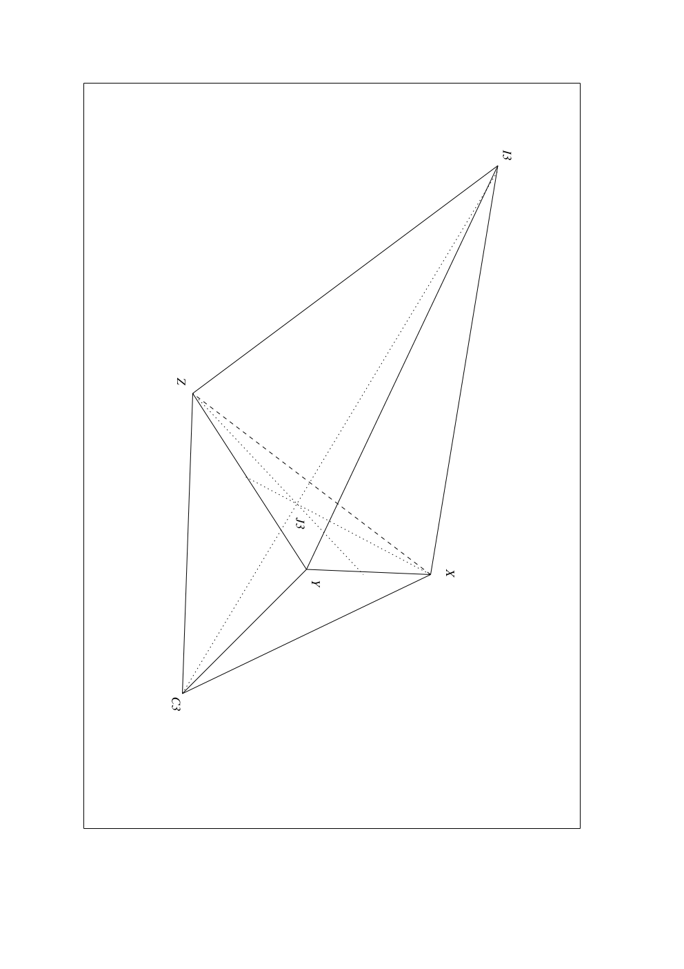
, and the triangle is equilateral with respect to the Frobenius norm. In addition, is an axis of symmetry for , and every point on commutes with all other points in .
Thus it is clear from the preceding lemma that is 3-dimensional and has the shape seen in Figure 1.
Our next goal is to prove that the only symmetric doubly stochastic matrices of (which is the closed triangle ) that are DS in are and its vertices and
Using Maple for example, it is easy to check the following lemma.
Lemma 3.2
For and with the symmetric doubly stochastic matrix has eigenvalues
Now if we let the domain be defined by and then it is easy to see that is the closed triangle whose vertices are and Define the function over by:
Concerning the function we have the following.
Lemma 3.3
Over the domain the function has zero as absolute minimum and 1 as an absolute maximum. Thus over the domain we have
Proof. Since is differentiable then the only places where can assume these values are points inside where the first partial derivatives satisfy and points on the boundary.
- 1.
Potential points inside : Solving the system
yields the unique solution with
- 2.
Potential points on the boundary of : We have to check the 3 sides of the triangle one side at a time.
1. On the segment which can be regarded as a function of where and such that its derivative for Therefore we have 3 potential points where their images by are given by and
2. On the segment clearly (as and play a symmetric role in the function ) we obtain the following potential points: and
3. On the segment we have already accounted for the values of at the endpoints of so that we only need to look at the interior points of Clearly and for Hence, is the final potential point with
Thus our claim is valid.
Remark 3.4
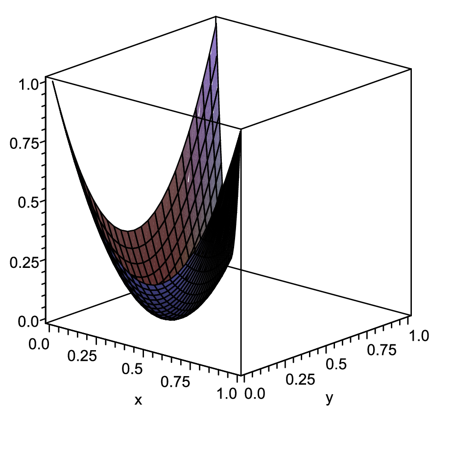
The surface where and any horizontal plane where intersect at exactly one point which is for and intersect at the three points and for Moreover, for they intersect in an infinite number of points (see Figure 2).
As a consequence, we have the following corollary.
Lemma 3.5
The only elements of that are DS in are and and
Proof. First note that the line segments and are permutationally similar as and are and any point outside these line segments can not be permutationally similar to a point on them (from the geometry of the triangle ). Let be any point in and consider the following two cases:
- 1.
If then for some Define where varies over the domain Then by the preceding lemma, Moreover, it is easy to check that the matrix given by has eigenvalues So that by Lemma 3.2 the two symmetric doubly stochastic matrices matrices and have the same spectrum. Since we are dealing with symmetric matrices, then they are similar. Thus in this case is not DS in
- 2.
For the case where is in without loss of generality let for some We want to show that there there exists which is similar to but not permutationally similar. For, let where varies over First the condition on in terms of for which and are similar is given by Such always exists due to the continuity of in Also we want to impose the other constraint that at least one entry of is not an entry of or vice versa so that they are not permutationally similar. Clearly and and since has at most two distinct entries which are and so that we need to impose the constraint that and An inspection shows that or if and only if or if and only if or So that our second constraint amounts to not being an element of Thus we only need to exclude these 3 particular values of and since then by Remark 3.4, an infinite number of such exists (since each of the 3 planes and intersects the curve in a finite number of points) so that we conclude that is not DS in
Finally, and are DS by Theorem 2.3 and is DS by Corollary 2.9.
For let intersect and in and respectively (for we only need to replace by in this statement). Then clearly is the closed triangle and the 3 vertices and are permutationally similar since and are. With these notations, we have the following.
Lemma 3.6
The only points of that are DS in are
Proof. For let be any point in and let the line through (resp. for ) and intersect in Clearly is in and is not DS by the preceding lemma. Then there exists in such that and are similar but not permutationally similar. Let be the intersection of (resp. for ) with then clearly and are similar but not permutationally similar.
If then is DS in Now if then it is enough to study the case where If there exists such that and are similar but not permutationally similar, then there exists such that and are similar but not permutationally similar which is a contradiction to being DS in
From the preceding 3 lemmas, we conclude one of our main results which completely solves Problem 1.4 in the case
Theorem 3.7
The only symmetric doubly stochastic matrices that are DS in are those lying on one of the following line-segments or
As a conclusion, we solve Problem 1.3 for the case
Corollary 3.8
The only points of that characterize permutationally elements of are those belonging to
Proof. It is enough to check that the spectrum of any of the 3 line-segments is and the spectrum of any of is The last part is true by Corollary 2.11.
4 Connections with spectral graph theory
In this section, we present some close connections between Problem 1.4 and the topic known “regular graphs that are DS” (see, e.g., [2, 6, 19, 20]).
First let us introduce some related notations (see, e.g. [1]). The adjacency matrix of a simple
graph will be denoted by which is a symmetric nonnegative (0,1)-matrix and its eigenvalues
form the spectrum of which is a multiset and will be
denoted by The graph is called integral if all of its eigenvalues are integers, and it is called circulant if is circulant. In addition, is said to be -regular if the degree of each of its vertices is A strongly regular graph with parameters is a -regular graph which is not complete nor edgeless and satisfying the following two conditions:
(i) For each pair of adjacent vertices there exist vertices adjacent to both.
(ii) For each pair of non-adjacent vertices there exist vertices adjacent to both.
We use the usual notation to denote the complete graph on vertices where each vertex is connected to all other vertices. Moreover, the complete bipartite graph has vertices partitioned into two subsets and of elements each, and two vertices are adjacent if and if only if one is in and the other is in
Two graphs are said to be isomorphic if and only if their adjacency matrices are permutationally similar. Two graphs are said to be cospectral or isospectral if they have the same spectrum. A graph is said to be DS if any graph which is cospectral to is isomorphic to In general, the problem of determining whether a graph is DS or not is still open though many partial results are known (see [20] for the latest developments on this problem).
We are particularly interested in the subproblem of finding which regular graphs are DS due to its link with Problem 1.4. To explain this, we need some more notations. But first recall that if is a -regular graph with vertices, then the spectral radius of equals and it is an eigenvalue of with corresponding unit eigenvector equals to Now let be the set of all nonnegative symmetric matrices with each row and each column equals to and denote the subset of formed by of all (0,1)-matrices with 1’s in each row and each column. In addition, let be the set of those elements of that have zero trace. Then clearly if and only if is the adjacency matrix of some -regular graph with vertices and edges. Also note that if is in if and only if is an element of So that if we extend the notion of DS to all elements of then obviously is DS in if and only if is DS in Also, note that a -regular graph is DS if and only if is DS in
It is well-known that 1-regular graphs are DS (see [6]); a fact that can be easily derived from Theorem 2.3. In addition, the fact that the complete graph is DS can be seen from Corollary 2.9 since On the one hand, a disjoint union of complete graphs is DS; a fact that can be deduced from Corollary 2.13, and on the other hand, is DS by Theorem 2.14.
Although proving that graphs are DS is a much more harder task than just showing they are not DS and the same is true for Problem 1.4, one can benefit from the fact that cospectral regular graphs that are not isomorphic (i.e. cospectral mates) give rise to symmetric doubly stochastic matrices that are not DS in So that all known results concerning finding cospectral mates for regular graphs can lead to exclude elements from as solutions to Problem 1.4. In what follows, we mention among the many such situations, 3 particular examples (see [2] for other situations). The first is concerned with strongly regular graphs where it is well known that connected strongly regular graphs with parameters have eigenvalue k appearing once and two other eigenvalues with prescribed multiplicity. In general there are many non-isomorphic graphs for a fixed parameter and the number of non-isomorphic graphs can grow dramatically (see e.g. [2]). The second deals with cospectral integral regular graphs where for example in [21](see also the references within) the authors prove the existence of infinitely many pairs of cospectral integral graphs which results in the existence of infinitely many pairs of symmetric doubly stochastic matrices that are not DS in The final case is concerned with circulant graphs (which are regular) where in [3] it is proved that there are infinitely many cospectral non-isomorphic circulant graphs.
5 Two related open questions and a conjecture
We conclude this paper with the following two open questions for which the answer to any of them can help shed some light on Problem 1.4 for general
(1) If is a -regular graph that is DS. Does this imply that is DS in ?
Note that as mentioned earlier this is true for 1-regular graphs, disjoint union of complete graphs, the graphs and
(2) What are the elements of that are DS in ?
we know that and the zero trace permutation matrices are among these ones.
Finally, based on the solution for the case we propose the following conjecture.
conjecture 5.1
For the only elements of that are DS in are points on the line segments and where is a vertex of
Acknowledgments
This work is supported by the Lebanese University research grants program for the Discrete Mathematics and Algebra research group.
References
- [1] R. B. Bapat, Graphs and Matrices, Springer, New York, 2010.
- [2] A. E. Brouwer, W. H. Haemers, Spectra of graphs, Springer, 2011.
- [3] J. Brown, Isomorphic and nonisomorphic, isospectral circulant graphs, available from arXiv:0904.1968v1, 2009.
- [4] R. Brualdi, From the Editor-in-chief, Lin. Alg. Appl., 434, (2011) pp. 449-853.
- [5] A. Cruse, A note on the symmetric doubly-stochastic matrices, Discrete Mathematics, 13, (1975) pp. 109-119.
- [6] D. Cvetkovi´c, P. Rowlinson, S. Simi´c, An introduction to the theory of graph spectra, Cambridge University Press, Cambridge, 2010.
- [7] M. Fang, A note on the inverse eigenvalue problem for symmetric doubly stochastic matrices, Lin. Alg. Appl., 432, issue 11, (2010) pp. 2925-2927.
- [8] S. G. Hwang and S. S. Pyo, The inverse eigenvalue problem for symmetric doubly stochastic matrices, Lin. Alg. Appl., 379, (2004) pp. 77-83.
- [9] C. R. Johnson, Row stochastic matrices similar to doubly-stochastic matrices, Lin. Multilin. Alg., 10, (1981) pp. 113-130.
- [10] I. Kaddoura and B. Mourad, On a conjecture concerning the inverse eigenvalue problem for symmetric doubly stochastic matrices, Int. Math. Forum 3, 31,(2008) pp. 1513-1519.
- [11] M. Katz, On the extreme points of a certain convex polytope, J. Combin. Theo., 8,(1970) pp.417-423.
- [12] H. Minc, Non-negative matrices, Berlin Press, New York, 1988.
- [13] B. Mourad, An inverse problem for symmetric doubly stochastic matrices, Inverse Problems, 19, (2003) pp. 821-831.
- [14] B. Mourad, On a Lie-theoretic approach to generalized doubly stochastic matrices and applications, Lin. and Multilin. Alg., 52, (2004) pp. 99-113.
- [15] B. Mourad, A note on the boundary of the set where the decreasingly ordered spectra of symmetric doubly stochastic matrices lie, Lin. Alg. Appl., 416, (2006) pp. 546-558.
- [16] B. Mourad, On a spectral property of doubly stochastic matrices and its application to their inverse eigenvalue problem, Lin. Alg. Appl., 436, (2012) pp. 3400-3412.
- [17] B. Mourad, H. Abbas, A. Mourad, A. Ghaddar and I. Kaddoura, An algorithm for constructing doubly stochastic matrices for the inverse eigenvalue problem, Lin. Alg. Appl., 439, (2013) pp. 1382-1400.
- [18] B. Mourad, Generalization of some results concerning eigenvalues of a certain class of matrices and some applications, Lin. and Multilin. Alg., (2012) DOI:10.1080/03081087.2012.746330.
- [19] E. R. Van Dam, W. H. Haemers, Which graphs are determined by their spectra, Lin. Alg. Appl., 373, (2003) pp. 241-272.
- [20] E. R. Van Dam, W. H. Haemers, Developments on spectral characterization of graphs, Discrete Math., 309, (2009) pp. 576-586.
- [21] L. G. Wang, H. Sun, Infinitely many pairs of cospectral integral regular graphs, App. Math. J., 26(3), (2011) pp. 280-286.
- [22] F. Zhang, Matrix theory: Basic results and techniques, Springer, New York, 1999.