Identifying Correlated Heavy-Hitters in a Two-Dimensional Data Stream

A preliminary version of the paper “Identifying Correlated Heavy-Hitters on a Two-Dimensional Data Stream” was accepted at the Proceedings of the 28th IEEE International Performance Computing and Communications Conference (IPCCC) 2009. The authors were supported in part by the National Science Foundation through grants NSF CNS-0834743 and CNS-0831903.

Bibudh Lahiri ^†^†thanks: Impetus Technologies, Los Gatos, CA 95032, USA. Email: bibudhlahiri@gmail.com Arko Provo Mukherjee ^†^†thanks: Department of Electrical and Computer Engineering, Iowa State University. Email: arko@iastate.edu Srikanta Tirthapura ^†^†thanks: Department of Electrical and Computer Engineering, Iowa State University. Email: snt@iastate.edu

Abstract

We consider online mining of correlated heavy-hitters from a data stream. Given a stream of two-dimensional data, a correlated aggregate query first extracts a substream by applying a predicate along a primary dimension, and then computes an aggregate along a secondary dimension. Prior work on identifying heavy-hitters in streams has almost exclusively focused on identifying heavy-hitters on a single dimensional stream, and these yield little insight into the properties of heavy-hitters along other dimensions. In typical applications however, an analyst is interested not only in identifying heavy-hitters, but also in understanding further properties such as: what other items appear frequently along with a heavy-hitter, or what is the frequency distribution of items that appear along with the heavy-hitters.

We consider queries of the following form: “In a stream $S$ of $(x,y)$ tuples, on the substream $H$ of all $x$ values that are heavy-hitters, maintain those $y$ values that occur frequently with the $x$ values in $H$ ”. We call this problem as Correlated Heavy-Hitters (CHH). We formulate an approximate formulation of CHH identification, and present an algorithm for tracking CHHs on a data stream. The algorithm is easy to implement and uses workspace which is orders of magnitude smaller than the stream itself. We present provable guarantees on the maximum error, as well as detailed experimental results that demonstrate the space-accuracy trade-off.

1 Introduction

Correlated aggregates [3, 16, 11] reveal interesting interactions among different attributes of a multi-dimensional dataset. They are useful in finding an aggregate on an attribute over a subset of the data, where the subset is defined by a selection predicate on a different attribute of the data. On stored data, a correlated aggregate can be computed by considering one dimension at a time, using multiple passes through the data. However, for dynamic streaming data, we often do not have the luxury of making multiple passes over the data, and moreover, the data may be too large to store and it is desirable to have an algorithm that works in a single pass through the data. Sometimes, even the substream derived by applying the query predicate along the primary dimension can be too large to store, let alone the whole dataset.

We first define the notion of a heavy-hitter on a data stream (this is considered in prior work, such as [21, 22, 7, 10]), and then define our notion of correlated heavy-hitters. Given a sequence of single-dimensional records $(a_{1},a_{2},\ldots,a_{N})$ , where $a_{i}\in\{1,\ldots,m\}$ , the frequency of an item $i$ is defined as $|\{a_{j}|a_{j}=i\}|$ . Given a user-input threshold $\phi\in(0,1)$ , any data item $i$ whose frequency is at least ${\phi}N$ is termed as a $\phi$ -heavy-hitter. We first consider the following problem of exact identification of CHHs.

Problem 1.

Exact Identification of Correlated Heavy Hitters. Given a data stream $S$ of $(x,y)$ tuples of length $N$ ( $x$ and $y$ will henceforth be referred to as the “primary” and the “secondary” dimensions, respectively), and two user-defined thresholds ${\phi}_{1}$ and ${\phi}_{2}$ , where $0<{\phi}_{1}<1$ and $0<{\phi}_{2}<1$ , identify all $(d,s)$ tuples such that:

f_{d}=|\{(x,y)\in S:(x=d)\}|>{{\phi}_{1}}N

and

f_{d,s}=|\{(x,y)\in S:(x=d)\land(y=s)\}|>{{\phi}_{2}}f_{d}

The above aggregate can be understood as follows. The elements $d$ are heavy-hitters in the traditional sense, on the stream formed by projecting along the primary dimension. For each heavy-hitter $d$ along the primary dimension, there is logically a (uni-dimensional) substream $S_{d}$ , consisting of all values along the secondary dimension, where the primary dimension equals $d$ . We require the tracking of all tuples $(d,s)$ such that $s$ is a heavy-hitter in $S_{d}$ .

Many stream mining and monitoring problems on two-dimensional streams need the CHH aggregate, and cannot be answered by independent aggregation along single dimensions. For example, consider a network monitoring application, where a stream of (destination IP address, source IP address) pairs is being observed. The network monitor maybe interested not only in tracking those destination IP addresses that receive a large fraction of traffic (heavy-hitter destinations), but also in tracking those source IP addresses that send a large volume of traffic to these heavy-hitter destinations. This cannot be done by independently tracking heavy-hitters along the primary and the secondary dimensions. Note that in this application, we are interested not only in the identity of the heavy-hitters, but also additional information on the substream induced by the heavy-hitters.

In another example, in a stream of (server IP address, port number) tuples, identifying the heavy-hitter server IP addresses will tell us which servers are popular, and identifying frequent port numbers (independently) will tell us which applications are popular; but a network manager maybe interested in knowing which applications are popular among the heavily loaded servers, which can be retrieved using a CHH query. Such correlation queries are used for network optimization and anomaly detection [12].

Another application is the recommendation system of a typical online shopping site, which shows a buyer a list of the items frequently bought with the ones she has decided to buy. Our algorithm can optimize the performance of such a system by parsing the transaction logs and identifying the items that were bought commonly with the frequently purchased items. If such information is stored in a cache with a small lookup time, then for most buyers, the recommendation system can save the time to perform a query on the disk-resident data.

Similar to the above examples, in many stream monitoring applications, it is important to track the heavy-hitters in the stream, but this monitoring should go beyond simple identification of heavy-hitters, or tracking their frequencies, as is considered in most prior formulations of heavy-hitter tracking such as [9, 21, 22, 7, 15]. In this work we initiate the study of tracking additional properties of heavy-hitters by considering tracking of correlated heavy hitters.

1.1 Approximate CHH

It is easy to prove that exact identification of heavy-hitters in a single dimension is impossible using limited space, and one pass through the input. Hence, the CHH problem is also impossible to solve in limited space, using a single pass through the input. Due to this, we consider the following approximate version of the problem. We introduce additional approximation parameters, ${\epsilon}_{1}$ and ${\epsilon}_{2}$ ( $0<{\epsilon}_{1}\leq\frac{{\phi}_{1}}{2}$ , $0<{\epsilon}_{2}<{\phi}_{2}$ ), which stand for the approximation errors along the primary and the secondary dimensions, respectively. We seek an algorithm that provides the following guarantees.

Problem 2.

Approximate Identification of Correlated Heavy-Hitters. Given a data stream $S$ of $(d,s)$ tuples of length $N$ , thresholds ${\phi}_{1}$ and ${\phi}_{2}$ :

1.

Report any value $d$ such that $f_{d}>{{\phi}_{1}}N$ as a heavy-hitter along the primary dimension.
2.

No value $d$ such that $f_{d}<({\phi}_{1}-{\epsilon}_{1})N$ , should be reported as a heavy-hitter along the primary dimension.
3.

For any value $d$ reported above, report any value $s$ along the secondary dimension such that $f_{d,s}>{{\phi}_{2}}f_{d}$ as a CHH.
4.

For any value $d$ reported above, no value $s$ along the secondary dimension such that $f_{d,s}<({{\phi}_{2}}-{{\epsilon}_{2}})f_{d}$ should be reported as a CHH occurring alongwith $d$ .

With this problem formulation, false positives are possible, but false negatives are not. In other words, if a pair $(d,s)$ is a CHH according to the definition in Problem 1, then it is a CHH according to the definition in Problem 2, and will be returned by the algorithm. But an algorithm for Problem 2 may return a pair $(d,s)$ that are not exact CHHs, but whose frequencies are close to the required thresholds.

1.2 Contributions

Our contributions are as follows.

•

We formulate exact and approximate versions of the problem of identifying CHHs in a multidimensional data stream, and present a small-space approximation algorithm for identifying approximate CHHs in a single pass. Prior literature on correlated aggregates have mostly focused on the correlated sum, and these techniques are not applicable for CHH. Our algorithm for approximate CHH identification is based on a nested application of the Misra-Gries algorithm [22].
•

We provide a provable guarantee on the approximation error. We show that there are no false negatives, and the error in the false positives is controlled. When greater memory is available, this error can be reduced. The space taken by the algorithm as well as the approximation error of the algorithm depend on the sizes of two different data structures within the algorithm. The total space taken by the sketch is minimized through solving a constrained optimization problem that minimizes the total space taken subject to providing the user-desired error guarantees.
•

We present results from our simulations on a) a stream of more than 1.4 billion (50 GB trace) anonymized packet headers from an OC48 link (collected by CAIDA [6]), and b) a sample of 240 million 2-grams extracted from English fiction books [18]. We compared the performance of our small-space algorithm with a slow, but exact algorithm that goes through the input data in multiple passes. Our experiments revealed that even with a space budget of a few megabytes, the average error of our algorithm was very small, showing that it is viable in practice.

Along each dimension our algorithm maintains frequency estimates of mostly those values (or pairs of values) that occur frequently. For example, in a stream of (destination IP, source IP) tuples, for every destination that sends a significant fraction of traffic on a link, we maintain mostly the sources that occur frequently along with this destination. Note that the set of heavy-hitters along the primary dimension can change as the stream elements arrive, and this influences the set of CHHs along the secondary dimension. For example, if an erstwhile heavy-hitter destination $d$ no longer qualifies as a heavy-hitter with increase in $N$ (and hence gets rejected from the sketch), then a source $s$ occurring with $d$ should also be discarded from the sketch. This interplay between different dimensions has to be handled carefully during algorithm design.

Roadmap: The rest of this paper is organized as follows. We present related work in Section 2. In Section 3.1 we present the algorithm description, followed by the proof of correctness in Section 3.2, and the analysis of the space complexity in Section 3.3. We present experimental results in Section 4.

2 Related Work

In the data streaming literature, there is a significant body of work on correlated aggregates ([3, 16, 11]), as well as on the identification of heavy hitters ([21, 22, 7, 10]). See [8] for a recent overview of work on heavy-hitter identification. None of these works consider correlated heavy-hitters.

Estan et al. [14] and Zhang et al. [26] have independently studied the problem of identifying heavy-hitters from multi-dimensional packet streams, but they both define a multidimensional tuple as a heavy-hitter if it occurs more than ${\phi}N$ times in the stream, $N$ being the stream size – the interplay across different dimensions is not considered.

There is significant prior work on correlated aggregate computation that we now describe. The problems considered in the literature usually take the following form. On a stream of two dimensional data items $(x,y)$ the query asks to first apply a selection predicate along the $x$ dimension, of the form $x\geq c$ or $x<c$ (for a value $c$ provided at query time), followed by an aggregation along the $y$ dimension. The difference when compared with this formulation is that in our case, the selection predicate along the $x$ dimension is one that involves frequencies and heavy-hitters, rather than a simple comparison.

Gehrke et al [16] addressed correlated aggregates where the aggregate along the primary dimension was an extremum (min or max) or the average, and the aggregate along the secondary dimension was sum or count. For example, given a stream $S$ of $(x,y)$ tuples, their algorithm could approximately answer queries of the following form: “Return the sum of $y$ -values from $S$ where the corresponding $x$ values are greater than a threshold $\alpha$ .” They describe a data structure called adaptive histograms, but these did not come with provable guarantees on performance. Ananthakrishna et al [3] presented algorithms with provable error bounds for correlated sum and count. Their solution was based on the quantile summary of [19]. With this technique, heavy-hitter queries cannot be used as the aggregate along the primary dimension since they cannot be computed on a stream using limited space. Cormode, Tirthapura, and Xu [11] presented algorithms for maintaining the more general case of time-decayed correlated aggregates, where the stream elements were weighted based on the time of arrival. This work also addressed the “sum” aggregate, and the methods are not directly applicable to heavy-hitters. Other work in this direction includes [5, 24]. Tirthapura and Woodruff [23] present a general method that reduces the correlated estimation of an aggregate to the streaming computation of the aggregate, for functions that admit sketches of a particular structure. These techniques only apply to selection predicates of the form $x>c$ or $x<c$ , and do not apply to heavy-hitters, as we consider here.

The heavy-hitters literature has usually focused on the following problem. Given a sequence of elements $A=(a_{1},a_{2},\ldots,a_{N})$ and a user-input threshold $\phi\in(0,1)$ , find data items that occur more than $\phi N$ times in $A$ . Misra and Gries [22] presented a deterministic algorithm for this problem, with space complexity being $O(\frac{1}{\phi})$ , time complexity for updating the sketch with the arrival of each element being $O(\log{\frac{1}{\phi}})$ , and query time complexity being $O(\frac{1}{\phi})$ . For exact identification of heavy-hitters, their algorithm works in two passes. For approximate heavy-hitters, their algorithm used only one pass through the sequence, and had the following approximation guarantee. Assume user-input threshold $\phi$ and approximation error $\epsilon<\phi$ . Note that for an online algorithm, $N$ is the number of elements received so far.

•

All items whose frequencies exceed ${\phi}N$ are output. i.e. there are no false negatives.
•

No item with frequency less than $(\phi-\epsilon)N$ is output.

Demaine et al [13] and Karp et al [20] improved the sketch update time per element of the Misra-Gries algorithm from $O(\log{\frac{1}{\phi}})$ to $O(1)$ , using an advanced data structure combining a hashtable, a linked list and a set of doubly-linked lists. Manku and Motwani [21] presented a deterministic “Lossy Counting” algorithm that offered the same approximation guarantees as the one-pass approximate Misra-Gries algorithm; but their algorithm required $O(\frac{1}{\epsilon}\log{({\epsilon}N)})$ space in the worst case. For our problem, we chose to extend the Misra-Gries algorithm as it takes asymptotically less space than [21].

3 Algorithm and Analysis

3.1 Intuition and Algorithm Description

Our algorithm is based on a nested application of an algorithm for identifying frequent items from an one-dimensional stream, due to Misra and Gries [22]. We first describe the Misra-Gries algorithm (henceforth called the MG algorithm). Suppose we are given an input stream $a_{1},a_{2},\ldots$ , and an error threshold $\epsilon,0<\epsilon<1$ . The algorithm maintains a data structure $\mathcal{D}$ that contains at most $\frac{1}{\epsilon}$ (key, count) pairs. On receiving an item $a_{i}$ , it is first checked if a tuple $(a_{i},\cdot)$ already exists in $\mathcal{D}$ . If it does, $a_{i}$ ’s count is incremented by 1; otherwise, the pair $(a_{i},1)$ is added to $\mathcal{D}$ . Now, if adding a new pair to $\mathcal{D}$ makes $|\mathcal{D}|$ exceed $\frac{1}{\epsilon}$ , then for each (key, count) pair in $\mathcal{D}$ , the count is decremented by one; and any key whose count falls to zero is discarded. This ensures at least the key which was most recently added (with a count of one) would get discarded, so the size of $\mathcal{D}$ , after processing all pairs, would come down to $\frac{1}{\epsilon}$ or less. Thus, the space requirement of this algorithm is $O(\frac{1}{\epsilon})$ . The data structure $\mathcal{D}$ can be implemented using hashtables or height-balanced binary search trees. At the end of one pass through the data, the MG algorithm maintains the frequencies of keys in the stream with an error of no more than $\epsilon n$ , where $n$ is the size of the stream. The MG algorithm can be used in exact identification of heavy hitters from a data stream using two passes through the data.

In the scenario of limited memory, the MG algorithm can be used to solve problem 1 in three passes through the data, as follows. We first describe a four pass algorithm. In the first two passes, heavy-hitters along the primary dimension are identified, using memory $O(1/{\phi}_{1})$ . Note that this is asymptotically the minimum possible memory requirement of any algorithm for identifying heavy-hitters, since the size of output can be $\Omega\left(\frac{1}{{\phi}_{1}}\right)$ . In the next two passes, heavy-hitters along the secondary dimension are identified for each heavy-hitter along the primary dimension. This takes space $O\left(\frac{1}{{\phi}_{2}}\right)$ for each heavy-hitter along the primary dimension. The total space cost is $O\left(\frac{1}{{{\phi}_{1}}{{\phi}_{2}}}\right)$ , which is optimal, since the output could be $\Omega\left(\frac{1}{{{\phi}_{1}}{{\phi}_{2}}}\right)$ elements. The above algorithm can be converted into a three pass exact algorithm by combining the second and third passes.

The high-level idea behind our single-pass algorithm for Problem 2 is as follows. The MG algorithm for an one-dimensional stream, can be viewed as maintaining a small space “sketch” of data that (approximately) maintains the frequencies of each distinct item $d$ along the primary dimension; of course, these frequency estimates are useful only for items that have very high frequencies. For each distinct item $d$ along the primary dimension, apart from maintaining its frequency estimate ${\hat{f}}_{d}$ , our algorithm maintains an embedded MG sketch of the substream $S_{d}$ induced by $d$ , i.e. $S_{d}=\{(x,y)|((x,y)\in S)\land(x=d)\}$ . The embedded sketch is a set of tuples of the form $(s,{\hat{f}}_{d,s})$ , where $s$ is an item that occurs in $S_{d}$ , and ${\hat{f}}_{d,s}$ is an estimate of the frequency of the pair $(d,s)$ in $S$ (or equivalently, the frequency of $s$ in $S_{d}$ ). While the actions on ${\hat{f}}_{d}$ (increment, decrement, discard) depend on how $d$ and the other items appear in $S$ , the actions on ${\hat{f}}_{d,s}$ depend on the items appearing in $S_{d}$ . Further, the sizes of the tables that are maintained have an important effect on both the correctness and the space complexity of the algorithm.

We now present a more detailed description. The algorithm maintains a table $H$ , which is a set of tuples $(d,{\hat{f}}_{d},H_{d})$ , where $d$ is a value along the primary dimension, ${\hat{f}}_{d}$ is the estimated frequency of $d$ in the stream, and $H_{d}$ is another table that stores the values of the secondary attribute that occur with $d$ . $H_{d}$ stores its content in the form of (key, count) pairs, where the keys are values ( $s$ ) along the secondary attribute and the counts are the frequencies of $s$ in $S_{d}$ , denoted as ${\hat{f}}_{d,s}$ , alongwith $d$ .

The maximum number of tuples in $H$ is $s_{1}$ , and the maximum number of tuples in each $H_{d}$ is $s_{2}$ . The values of $s_{1}$ and $s_{2}$ depend on the parameters $\phi_{1},\phi_{2},\epsilon_{1},\epsilon_{2}$ , and are decided at the start of the algorithm. Since $s_{1}$ and $s_{2}$ effect the space complexity of the algorithm, as well as the correctness guarantees provided by it, their values are set based on an optimization procedure, as described in Section 3.3.

The formal description is presented in Algorithms 1, 2 and 3. Before a stream element is received, Algorithm 1 Sketch-Initialize is invoked to initialize the data structures. Algorithm 2 Sketch-Update is invoked to update the data structure as each stream tuple $(x,y)$ arrives. Algorithm 3 Report-CHH is used to answer queries when a user asks for the CHHs in the stream so far.

On receiving an element $(x,y)$ of the stream, the following three scenarios may arise. We explain the action taken in each.

1.

If $x$ is present in $H$ , and $y$ is present in $H_{x}$ , then both ${\hat{f}}_{x}$ and ${\hat{f}}_{x,y}$ are incremented.
2.

If $x$ is present in $H$ , but $y$ is not in $H_{x}$ , then $y$ is added to $H_{x}$ with a count of 1. If this addition causes $|H_{x}|$ to exceed its space budget $s_{2}$ , then for each (key, count) pair in $H_{x}$ , the count is decremented by 1 (similar to the MG algorithm). If the count of any key falls to zero, the key is dropped from $H_{x}$ . Note that after this operation, the size of $H_{x}$ will be at most $s_{2}$ .
3.

If $x$ is not present in $H$ , then an entry is created for $x$ in $H$ by setting ${\hat{f}}_{x}$ to 1, and by initializing $H_{x}$ with the pair $(y,1)$ . If adding this entry causes $|H|$ to exceed $s_{1}$ , then for each $d\in H$ , $f_{d}$ is decremented by $1$ . If the decrement causes ${\hat{f}}_{d}$ to be zero, then we simply discard the entry for $d$ from $H$ .

Otherwise, when $f_{d}$ is decremented, the algorithm keeps the sum of the $\hat{f_{d,s}}$ counts within $H_{d}$ equal to $f_{d}$ ; the detailed correctness is proved in Section 3.3. To achieve this, an arbitrary key $s$ is selected from $H_{d}$ such that such that ${\hat{f}}_{d,s}>0$ , and ${\hat{f}}_{d,s}$ is decremented by $1$ . If ${\hat{f}}_{d,s}$ falls to zero, $s$ is discarded from $H_{d}$ .

Algorithm 1 Sketch-Initialize

({\phi}_{1},{\phi}_{2},{\epsilon}_{1},{\epsilon}_{2})

Input: Threshold for primary dimension

{\phi}_{1}

; Threshold for secondary dimension

{\phi}_{2}

; Tolerance for primary dimension

{\epsilon}_{1}

; Tolerance for secondary dimension

{\epsilon}_{2}

H\leftarrow\Phi

2 Set

s_{1}

and

s_{2}

as described in Section 3.3.

Algorithm 2 Sketch-Update

(x,y)

Input: Element along primary dimension

x

; Element along secondary dimension

y

1 if $x\in H$ then

{\hat{f}}_{x}\leftarrow{\hat{f}}_{x}+1

;

3 if $y\in H_{x}$ then

4 /* Both

x

and

y

are present */

5 Increment

{\hat{f}}_{x,y}

H_{x}

by 1;

6 else

7 /*

x\in H

, but

y\not\in H_{x}

8 Add the tuple

(y,1)

H_{x}

;

9 if $|H_{x}|>s_{2}$ then

10 foreach $(s,{\hat{f}}_{d,s})\in H_{x}$ do

{\hat{f}}_{d,s}\leftarrow{\hat{f}}_{d,s}-1

;

12 if ${\hat{f}}_{d,s}=0$ then

13 discard

(s,{\hat{f}}_{d,s})

from

H_{x}

;

14 else

15 /* Neither of

x

y

is present */

H_{x}\leftarrow\Phi

; Add

(y,1)

H_{x}

;

{\hat{f}}_{x}\leftarrow 1

;

17 if $|H|>s_{1}$ then

18 foreach $d\in H$ do

{\hat{f}}_{d}\leftarrow{\hat{f}}_{d}-1

;

20 if there exists $s$ such that ${\hat{f}}_{d,s}>0$ then

21 Choose an arbitrary

(s,{\hat{f}}_{d,s})\in H_{d}

such that

{\hat{f}}_{d,s}>0

;

{\hat{f}}_{d,s}\leftarrow{\hat{f}}_{d,s}-1

;

23 if ${\hat{f}}_{d,s}=0$ then

24 discard

(s,{\hat{f}}_{d,s})

from

H_{d}

;

25 if ${\hat{f}}_{d}=0$ then

26 Discard

(d,H_{d})

from

H

;

Algorithm 3 Report-CHH(

N

)

Input: Size of the stream

N

1 foreach $d\in H$ do

2 if ${\hat{f}}_{d}\geq({\phi}_{1}-\frac{1}{s_{1}})N$ then

3 Report

d

as a frequent value of the primary attribute;

4 foreach $(s,{\hat{f}}_{d,s})\in H_{d}$ do

5 if ${\hat{f}}_{d,s}\geq({\phi}_{2}-\frac{1}{s_{2}}){\hat{f}}_{d}-\frac{N}{s_{1}}$ then

6 Report

s

as a CHH occurring with

d

;

3.2 Algorithm Correctness

In this section, we show the correctness of the algorithm, subject to the following constraints on $s_{1}$ and $s_{2}$ . In Section 3.3, we assign values to $s_{1}$ and $s_{2}$ in such a manner that the space taken by the data structure is minimized.

Constraint 1.

\frac{1}{s_{1}}\leq{\epsilon}_{1}

Constraint 2.

\frac{1}{s_{2}}+\frac{1+{\phi}_{2}}{s_{1}({\phi}_{1}-{\epsilon}_{1})}\leq{\epsilon}_{2}

Consider the state of the data structure after a stream $S$ of length $N$ has been observed. Consider a value $d$ of the primary attribute, and $s$ of the secondary attribute. Let $f_{d}$ and $f_{d,s}$ be defined as in Section 1. Our analysis focuses on the values of variables $\hat{f}_{d}$ and $\hat{f}_{d,s}$ , which are updated in Algorithms 2 and used in Algorithm 3. For convenience, if $d$ is not present in $H$ then we define $\hat{f}_{d}=0$ . Similarly, if $d$ is not present in $H$ , or if $(d,s)$ is not present in $H_{d}$ , then we define $\hat{f}_{d,s}=0$ .

Lemma 1.

\hat{f}_{d}\geq f_{d}-\frac{N}{s_{1}}

Proof.

The total number of increments in the $s_{1}$ counters that keep track of the counts of the different values of the primary attribute is $N$ . Each time there is a decrement to $\hat{f}_{d}$ (in Line 20 of Algorithm 2), $s_{1}+1$ different counters are decremented. The total number of decrements, however, cannot be more than the total number of increments, and hence is at most $N$ . So the number of times the block of lines 19-31 in Algorithm 2 gets executed is at most $\frac{N}{s_{1}+1}<\frac{N}{s_{1}}$ . We also know that $\hat{f}_{d}$ is incremented exactly $f_{d}$ times, hence the final value of $\hat{f}_{d}$ is greater than $f_{d}-\frac{N}{s_{1}}$ . ∎

Lemma 2.

Assume that Constraint 1 is true. If $f_{d}>{\phi}_{1}N$ , then $d$ is reported by Algorithm 3 as a frequent item. Further, if $f_{d}<(\phi_{1}-\epsilon_{1})N$ , then $d$ is not reported as a frequent item.

Proof.

Suppose $f_{d}\geq\phi_{1}N$ . From Lemma 1, $\hat{f}_{d}\geq f_{d}-{\epsilon}_{1}N\geq{{\phi}_{1}}N-{\epsilon}_{1}N$ . Hence Algorithm 3 will report $d$ (see Lines 2 and 3). Next, suppose that $f_{d}<(\phi_{1}-\epsilon_{1})N$ . Since $\hat{f}_{d}\leq f_{d}$ , Algorithm 3 will not report $d$ as a frequent item. ∎

Lemma 3.

\sum_{(s,\cdot)\in H_{d}}\hat{f}_{d,s}\leq\hat{f}_{d}

Proof.

Let $\Sigma_{d}=\sum_{(s,\cdot)\in H_{d}}\hat{f}_{d,s}$ . Let $C(n)$ denote the condition $\Sigma_{d}\leq\hat{f}_{d}$ after $n$ stream elements have been observed. We prove $C(n)$ by induction on $n$ . The base case is when $n=0$ , and in this case, $\hat{f}_{d,s}=\hat{f}_{d}=0$ for all $d,s$ , and $C(0)$ is trivially true. For the inductive step, assume that $C(k)$ is true, for $k\geq 0$ . Consider a new element that arrives, say $(x,y)$ , and consider Algorithm 2 applied on this element. We consider four possible cases.

(I) If $x=d$ , and $d\in H$ , then $\hat{f}_{d}$ is incremented by $1$ , and it can be verified (Lines 3-11) that $\Sigma_{d}$ increases by at most $1$ (and may even decrease). Thus $C(k+1)$ is true.

(II) If $x=d$ , and $d\not\in H$ , then initially, $\hat{f}_{d}$ and $\Sigma_{d}$ are both 1 (line 17). If $|H|\leq s_{1}$ , then both $\hat{f}_{d}$ and $\Sigma_{d}$ remain 1, and $C(k+1)$ is true. Suppose $|H|>s_{1}$ , then both $\hat{f}_{d}$ and $\Sigma_{d}$ will go down to $0$ , since $H_{d}$ will be discarded from $H$ . Thus $C(k+1)$ is true.

(III) If $x\neq d$ , and $x\in H$ , then neither $\hat{f}_{d}$ nor $\Sigma_{d}$ change.

(IV) Finally, if $x\neq d$ and $x\not\in H$ , then it is possible that $\hat{f}_{d}$ is decremented (line 20). In this case, if $\Sigma_{d}>0$ , then $\Sigma_{d}$ is also decremented (line 22), and $C(k+1)$ is satisfied. If $\Sigma_{d}=0$ , then $C(k+1)$ is trivially satisfied since $\hat{f}_{d}\geq 0$ . ∎

Lemma 4.

Subject to Constraint 1, $\hat{f}_{d,s}\geq f_{d,s}-\epsilon_{2}f_{d}-\epsilon_{1}N$ .

Proof.

Note that each time the tuple $(d,s)$ occurs in the stream, $\hat{f}_{d,s}$ is incremented in Algorithm 2. But $\hat{f}_{d,s}$ can be less than $f_{d,s}$ because of decrements in Lines 2 or 2 in Algorithm 2. We consider these two cases separately.

Let $\Sigma_{d}=\sum_{(s,\cdot)\in H_{d}}\hat{f}_{d,s}$ . For decrements in Line 9, we observe that each time this line is executed, $\Sigma_{d}$ reduces by $s_{2}+1$ . From Lemma 3, we know that $\Sigma_{d}\leq\hat{f}_{d}\leq f_{d}$ . Thus the total number of times $\hat{f}_{d,s}$ is decremented due to Line 9 is no more than $\frac{f_{d}}{s_{2}+1}$ . From Constraint 2, we know $\frac{1}{s_{2}}<\epsilon_{2}$ , and $\frac{f_{d}}{s_{2}+1}<\epsilon_{2}f_{d}$ .

For decrements in Line 23, we observe that $\hat{f}_{d,s}$ is decremented in Line 23 no more than the number of decrements to $\hat{f}_{d}$ , which was bounded by $\frac{N}{s_{1}}$ in Lemma 1. From Constraint 1, this is no more than $\epsilon_{1}N$ . ∎

Lemma 5.

For any value $d$ that gets reported in line 3 of Algorithm 3, any value $s$ of the secondary attribute that occurs with $d$ such that $f_{d,s}>\phi_{2}f_{d}$ , will be identified by line 6 of Algorithm 3 as a CHH occurring alongwith $d$ .

Proof.

From Lemma 4,

$\displaystyle\hat{f}_{d,s}$	$\displaystyle\geq$	$\displaystyle f_{d,s}-{{\epsilon}_{2}}f_{d}-{{\epsilon}_{1}}N$
	$\displaystyle>$	$\displaystyle{{\phi}_{2}}f_{d}-{{\epsilon}_{2}}f_{d}-{{\epsilon}_{1}}N$
	$\displaystyle=$	$\displaystyle({\phi}_{2}-{\epsilon}_{2})f_{d}-{\epsilon}_{1}N$
	$\displaystyle\geq$	$\displaystyle({\phi}_{2}-{\epsilon}_{2}){\hat{f}}_{d}-{\epsilon}_{1}N$

where we have used $f_{d}\geq\hat{f}_{d}$ . The lemma follows since $({\phi}_{2}-{\epsilon}_{2}){\hat{f}}_{d}-{\epsilon}_{1}N$ is the threshold used in line 5 of Algorithm 3 to report a value of the secondary attribute as a CHH. ∎

Lemma 6.

Under Constraints 1 and 2, for any value of $d$ that is reported as a heavy-hitter along the primary dimension, then for a value $s^{\prime}$ along the secondary dimension, if $f_{d,s^{\prime}}<(\phi_{2}-\epsilon_{2})f_{d}$ , then the pair $(d,s^{\prime})$ will not be reported as a CHH.

Proof.

We will prove the contrapositive of the above statement. Consider a value $s$ such that $(d,s)$ is reported as a CHH. Then, we show that $f_{d,s}\geq(\phi_{2}-\epsilon_{2})f_{d}$ .

If $(d,s)$ is reported, then it must be true that $\hat{f}_{d,s}\geq(\phi_{2}-\frac{1}{s_{2}})\hat{f}_{d}-\frac{N}{s_{1}}$ (Algorithm 3, line 5). Using $f_{d,s}\geq\hat{f}_{d,s}$ , and $\hat{f}_{d}\geq f_{d}-\frac{N}{s_{1}}$ , we get:

$\displaystyle f_{d,s}$	$\displaystyle\geq$	$\displaystyle\hat{f}_{d,s}$
	$\displaystyle\geq$	$\displaystyle(\phi_{2}-\frac{1}{s_{2}})\hat{f}_{d}-\frac{N}{s_{1}}$
	$\displaystyle\geq$	$\displaystyle(\phi_{2}-\frac{1}{s_{2}})(f_{d}-\frac{N}{s_{1}})-\frac{N}{s_{1}}$
	$\displaystyle=$	$\displaystyle(\phi_{2}-\frac{1}{s_{2}})f_{d}-\frac{N}{s_{1}}\left(1+{\phi}_{2}-\frac{1}{s_{2}}\right)$
	$\displaystyle\geq$	$\displaystyle({\phi}_{2}-\frac{1}{s_{2}})f_{d}-\frac{f_{d}}{({\phi}_{1}-{\epsilon}_{1})s_{1}}\left(1+{\phi}_{2}-\frac{1}{s_{2}}\right)$
		(since $d$ gets reported, by Lemma 2, $f_{d}\geq({\phi}_{1}-{\epsilon}_{1})N\Rightarrow N\leq\frac{f_{d}}{{\phi}_{1}-{\epsilon}_{1}}$ )
	$\displaystyle=$	$\displaystyle\left({\phi}_{2}-\frac{1}{s_{2}}-\frac{1}{({\phi}_{1}-{\epsilon}_{1})s_{1}}\left(1+{\phi}_{2}-\frac{1}{s_{2}}\right)\right)f_{d}$
	$\displaystyle\geq$	$\displaystyle f_{d}({\phi}_{2}-{\epsilon}_{2})\mbox{(using Constraint~\ref{const:s1s2})}$

∎

Lemmas 6, 5, and 2 together yield the following.

Theorem 1.

If Constraints 1 and 2 are satisfied, then Algorithms 1, 2 and 3 satisfy all the four requirements of Problem 2.

3.3 Analysis

We analyze the space complexity of the algorithm. In Theorem 1, we showed that the Algorithms 2 and 3 solve the Approximate CHH detection problem, as long as constraints 1 and 2 are satisfied.

Space Complexity in terms of $s_{1}$ and $s_{2}$ . In our algorithm, we maintain at most $s_{2}$ counters for each of the (at most) $s_{1}$ distinct values of the primary attribute in $H$ . Hence, the size of our sketch is $O(s_{1}+s_{1}s_{2})=O(s_{1}s_{2})$ . We now focus on the following question. What is the setting of $s_{1}$ and $s_{2}$ so that the space complexity of the sketch is minimized while meeting the constraints required for correctness.?

Lemma 7.

Let $\alpha=\left(\frac{1+{\phi}_{2}}{{\phi}_{1}-{\epsilon}_{1}}\right)$ . Subject to constraints 1 and 2, the space of the data structure is minimized by the following settings of $s_{1}$ and $s_{2}$ .

•

If $\epsilon_{1}\geq\frac{\epsilon_{2}}{2\alpha}$ , then $s_{1}=\frac{2\alpha}{\epsilon}$ and $s_{2}=\frac{2}{\epsilon_{2}}$ . In this case, the space complexity is $O\left(\frac{1}{(\phi_{1}-\epsilon_{1})\epsilon_{2}^{2}}\right)$ .
•

If $\epsilon_{1}<\frac{\epsilon_{2}}{2\alpha}$ , then $s_{1}=\frac{1}{\epsilon_{1}}$ , and $s_{2}=\frac{1}{\epsilon_{2}-\alpha\epsilon_{1}}$ . In this case, the space complexity is $O(\frac{1}{\epsilon_{1}\epsilon_{2}})$ .

Proof.

Let $\sigma_{1}=\frac{1}{s_{1}}$ , $\sigma_{2}=\frac{1}{s_{2}}$ . The problem is now to maximize $\sigma_{1}\sigma_{2}$ . Constraints 1 and 2 can be rewritten as follows.

•

Constraint 1: $\sigma_{1}\leq\epsilon_{1}$
•

Constraint 2: $\alpha\sigma_{1}+{\sigma}_{2}\leq{\epsilon}_{2}$

First, we note that any assignment $(\sigma_{1},\sigma_{2})=(x,y)$ that maximizes $\sigma_{1}\sigma_{2}$ must be tight on Constraint 2, i.e. $\alpha x+y=\epsilon_{2}$ . This can be proved by contradiction. Suppose not, and $\alpha x+y<\epsilon_{2}$ , and $xy$ is the maximum possible. Now, there is a solution $\sigma_{1}=x$ , and $\sigma_{2}=y^{\prime}$ , such that $y<y^{\prime}$ , and Constraints 1 and 2 are still satisfied. Further, $xy^{\prime}>xy$ , showing that the solution $(x,y)$ is not optimal.

Thus, we have:

\sigma_{2}=\epsilon_{2}-\alpha\sigma_{1}

(1)

Thus the problem has reduced to: Maximize $f(\sigma_{1})=\sigma_{1}\left(\epsilon_{2}-\alpha\sigma_{1}\right)$ subject to $\sigma_{1}\leq\epsilon_{1}$ .

Consider

f^{\prime}(\sigma_{1})=\epsilon_{2}-2\alpha\sigma_{1}

We consider two cases.

•

Case I: $\epsilon_{1}\geq\frac{\epsilon_{2}}{2\alpha}$ .

Setting $f^{\prime}(\sigma_{1})=0$ , we find that the function reaches a fixed point at $\sigma_{1}=\frac{\epsilon_{2}}{2\alpha}$ . At this point, $f^{\prime\prime}(\sigma_{1})=-2\alpha$ , which is negative. Hence $f(\sigma_{1})$ is maximized at $\sigma_{1}=\frac{\epsilon_{2}}{2\alpha}$ . We note that this value of $\sigma_{1}$ does not violate Constraint 1, and hence this is a feasible solution. In this case, the optimal settings are: $\sigma_{1}=\frac{\epsilon_{2}}{2\alpha}$ and $\sigma_{2}=\frac{\epsilon_{2}}{2}$ . Thus $s_{1}=\frac{2\alpha}{\epsilon}$ and $s_{2}=\frac{2}{\epsilon_{2}}$ . The space complexity is $O(\frac{1}{\sigma_{1}\sigma_{2}})=O(\frac{4\alpha}{\epsilon_{2}^{2}})$ .
•

Case II: $\epsilon_{1}<\frac{\epsilon_{2}}{2\alpha}$

The function $f(\sigma_{1})$ is increasing for $\sigma_{1}$ from $0$ to $\frac{\epsilon_{2}}{2\alpha}$ . Hence this will be maximized at the point $\sigma_{1}=\epsilon_{1}$ . Thus, in this case the optimal settings are $\sigma_{1}=\epsilon_{1}$ , and $\sigma_{2}=\epsilon_{2}-\alpha\epsilon_{1}$ . Thus, $s_{1}=\frac{1}{\epsilon_{1}}$ , and $s_{2}=\frac{1}{\epsilon_{2}-\alpha\epsilon_{1}}$ . The space complexity is: $O(\frac{1}{\epsilon_{1}(\epsilon_{2}-\alpha\epsilon_{1})})$ .

We note that since $\epsilon_{2}>2\alpha\epsilon_{1}$ , we have $(\epsilon_{2}-\alpha\epsilon_{1})>\frac{\epsilon_{2}}{2}$ , and hence the space complexity is $O(\frac{1}{\epsilon_{1}\epsilon_{2}})$ .

∎

Lemma 8.

The time taken to update the sketch on receiving each element of the stream is $O(\max(s_{1},s_{2}))$ .

Proof.

In processing an element $(x,y)$ of the stream by Algorithm 2, the following three scenarios may arise.

1.

$x$ is present in $H$ , and $y$ is present in $H_{x}$ . We implemented the tables as hash tables, hence the time taken to look up and increment ${\hat{f}}_{x}$ from $H$ and ${\hat{f}}_{x,y}$ from $H_{x}$ is O(1).
2.

$x$ is present in $H$ , but $y$ is not in $H_{x}$ . If the size of $H_{x}$ exceeds its space budget $s_{2}$ , then, the time taken to decrement the frequencies of all the stored values of the secondary attribute is $O(s_{2})$ .
3.

$x$ is not present in $H$ . If the size of $H$ exceeds its space budget $s_{1}$ , then the time taken to decrement the frequencies of all the stored values of the primary attribute is $O(s_{1})$ .

The time complexity to update the sketch on receiving each element is the maximum of these three, which establishes the claim. ∎

4 Experiments

We simulated our algorithm for finding correlated heavy-hitters in C++, using the APIs offered by the Standard Template Library [1], on three different datasets:

•

IPPair: An anonymized packet header trace collected by CAIDA [6] in both directions of an OC48 link. We used windump [2] in conjunction with a custom Java application to extract the source IP address, the destination IP address, the source port number and the destination port number from the .pcap files. Then, we took the comibation of (destination IP, source IP) tuples to create this dataset. “IPPair” had 1.4 billion such tuples.
•

PortIP: This is generated from the same trace as “IPPair”, but it is a sample of 20.7 million (destination port, destination IP) tuples.
•

NGram: It is the “English fiction” 2-grams dataset based on the Google n-gram dataset [18]. This is a collection of 2-grams extracted from books predominantly in the English language that a library or publisher identified as fiction. Some of the interesting trend analysis of 2-grams in English fiction can be found here [17], e.g., the 2-gram “child care” started replacing the 2-gram “nursery school” in the mid-1970s. We took a uniform random sample of this dataset. We will refer to the two elements of a tuple as the “first gram” and the “second gram” respectively.

Objective: The goal of the simulation was threefold: first, to learn about typical frequency distributions along both the dimensions in real two-dimensional data streams; second, to illustrate the reduction in space and time cost achievable by the small-space algorithm in practice; and finally, to demonstrate how the space budget (and hence, the allocated memory) influences the accuracy of our algorithm in practice.

For the first objective, we ran a naive algorithm on a smaller sample of size 248 million taken from the “IPPair” dataset, where all the distinct destination IPs were stored, and for each distinct destination IP, all the distinct source IPs were stored. We identified (exactly) the frequent values along both the dimensions for ${\phi}_{1}=0.001$ and ${\phi}_{2}=0.001$ . Only 43 of the 1.2 million distinct destination IPs were reported as heavy-hitters. For the secondary dimension, we ranked the heavy-hitter destination IPs based on the number of distinct source IPs they co-occurred with, and the number of distinct source IPs for the top eight are shown in Figure 1. All these heavy-hitter destination IPs co-occurred with 9,000-18,000 distinct source IPs, whereas, for all of them, the number of co-occurring heavy-hitter source IPs was in the range 20-200 (note that the Y-axis in Figure 1 is in log scale). This shows that the distribution of the primary attribute values, as well as that of the secondary attribute values for a given value of the primary attribute, are very skewed, and hence call for the design of small-space approximation algorithms like ours.

We did a similar exercise for the “NGram” dataset, and the result is in Figure 2. Once again, the values of ${\phi}_{1}$ and ${\phi}_{2}$ were both 0.001, and note that the number of distinct second grams, co-occurring with the first grams, varies between 10 million and 100 million, but the number of CHH second grams vary between 10 and 100 only, orders of magnitude lower than the number of distinct values of the second grams.

Since the “NGram” dataset is based on English fiction text, we observed some interesting patterns while working with the dataset: pairs of words that occur frequently together, as reported by this dataset, are indeed words whose co-occurrence intuitively look natural. We present some examples in Table 1, alongwith their frequencies:

Table 1: Pairs of words frequently occurring together

Gram1	Frequency of Gram1	Gram2	Frequency of Gram2 alongwith Gram1
are	1989774	hardly	4717
are	1989774	meant	5031
still	1601172	remained	4798
out	1777906	everything	5497
was	2373607	present	7932
was	2373607	deserted	7641
look	1226326	outside	2052
could	1215055	suggest	5081

Refer to caption — Figure 1: Basic statistics for a sample of “IPPair”. On the X-axis are the ranks of the eight (heavy-hitter) destination IPs, that co-appear with maximum number of distinct source IPs. For each destination IP, the Y-axis shows 1) the number of distinct source IPs co-occurring with it, 2) the number of heavy-hitter destination IPs co-appearing with it. Note that the Y-axis is logarithmic.

The second objective was accomplished by comparing the space and time costs of the naive algorithm as above (on the same sample of size 248 million taken from the “IPPair” dataset), with those of the small-space algorithm, run with $s_{1}=3000$ and $s_{2}=2000$ (Figure 3). We defined the space cost as the distinct number of (dstIP, srcIP) tuples stored $\left(\sum_{d}|H_{d}|\right)$ , which is 34 times higher for the naive algorithm compared to the small-space one. Also, the naive algorithm took more than twice as much time to run the small-space one.

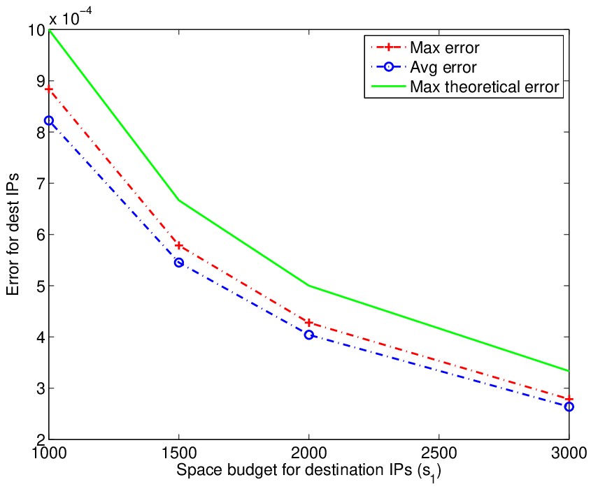
For the third objective, we tested the small-space algorithm on all three datasets (with different values of $s_{1}$ and $s_{2}$ ): “IPPair”, “PortIP” and “NGram”. To test the accuracy of our small-space algorithm, we derived the “ground truth”, i.e., a list of the actual heavy-hitters along both the dimensions along with their exact frequencies, by employing a four-pass variant of the Misra-Gries algorithm (as discussed in Section 1.1).

Observations: We define the error statistic in estimating the frequency of a heavy-hitter value $d$ of the primary attribute as $\frac{f_{d}-{\hat{f}}_{d}}{N}$ , and in Figures 4, 6 and 8, for each value of $s_{1}$ , we plot the maximum and the average of this error statistic over all the heavy-hitter values of the primary attribute. We observed that both the maximum and the average fell sharply as $s_{1}$ increased. Even by using a space budget ( $s_{1}$ ) as low as 1000, the maximum error statistic was only 0.09% for “IPPair”, 0.04% for “PortIP” and 0.03% for “NGram”.

The graphs in Figures 5, 7 and 9 show the results of running our small-space algorithm with different values of $s_{1}$ as well as $s_{2}$ . We define the error statistic in estimating the frequency of a CHH $s$ (that occurs alongwith a heavy-hitter primary attribute $d$ ) as $\frac{f_{d,s}-{\hat{f}}_{d,s}}{f_{d}}$ , and for each combination of $s_{1}$ and $s_{2}$ , we plot the theoretical maximum, the experimental maximum and the average of this error statistic over all CHH attributes. Here also, we observed that both the maximum and the average fall sharply as $s_{1}$ increases. However, for a fixed value of $s_{1}$ , as we increased the value of $s_{2}$ , the maximum did not change at all (for either of three datasets), and the average did not reduce too much - this becomes evident if we compare the readings of the three sub-figures in Figures 5, 7 and 9, which differ in their values of $s_{2}$ , for identical values of $s_{1}$ . The possible reason is the number of CHHs being very low compared to the number of distinct values of the secondary attribute occurring with a heavy-hitter primary attribute, as we have pointed out in Figure 1 for “IPPair” and Figure 2 for “NGram”. However, this is good because it implies that in practice, setting $s_{2}$ as low as $\frac{1}{{\phi}_{2}}$ should be enough.

5 Conclusion and Future Work

For two-dimensional data streams, we presented a small-space approximation algorithm to identify the heavy-hitters along the secondary dimension from the substreams induced by the heavy-hitters along the primary. We theoretically studied the relationship between the maximum errors in the frequency estimates of the heavy-hitters and the space budgets; computed the minimum space requirement along the two dimensions for user-given error bounds; and tested our algorithm to show the space-accuracy tradeoff for both the dimensions.

Identifying the heavy-hitters along any one dimension allows us to split the original stream into several important substreams; and take a closer look at each one to identify the properties of the heavy-hitters. In future, we plan to work on computing other statistics of the heavy-hitters. For example, as we have already discussed in Section 4, our experiments with the naive algorithm (on both the datasets) revealed that the number of distinct secondary attribute values varied quite significantly across the different (heavy-hitter) values of the primary attribute. For any such data with high variance, estimating the variance in small space [4, 25] is an interesting problem in itself. Moreover, for data with high variance, the simple arithmetic mean is not an ideal central measure, so finding different quantiles, once again in small space, can be another problem worth studying.

References

[1] http://www.sgi.com/tech/stl/.
[2] http://www.winpcap.org.
[3] Rohit Ananthakrishna, Abhinandan Das, Johannes Gehrke, Flip Korn, S. Muthukrishnan, and Divesh Srivastava. Efficient approximation of correlated sums on data streams. IEEE Transactions on Knowledge and Data Engineering, 15(3):569–572, 2003.
[4] Brian Babcock, Mayur Datar, Rajeev Motwani, and Liadan O’Callaghan. Maintaining variance and k-medians over data stream windows. In Proceedings of the Twenty-Second ACM SIGACT-SIGMOD-SIGART Symposium on Principles of Database Systems (PODS), pages 234–243, 2003.
[5] C. Busch and S. Tirthapura. A deterministic algorithm for summarizing asynchronous streams over a sliding window. In STACS, 2007.
[6] CAIDA. OC48 traces dataset. https://data.caida.org/datasets/oc48/oc48-original/20020814/5min/.
[7] Moses Charikar, Kevin Chen, and Martin Farach-Colton. Finding frequent items in data streams. Theoretical Computer Science, 312(1):3–15, 2004.
[8] Graham Cormode and Marios Hadjieleftheriou. Finding the frequent items in streams of data. Commun. ACM, 52(10):97–105, 2009.
[9] Graham Cormode and S. Muthukrishnan. What’s hot and what’s not: tracking most frequent items dynamically. In Proceedings of the 22nd ACM SIGMOD International Conference on Management of Data / Principles of Database Systems (PODS), pages 296–306, 2003.
[10] Graham Cormode and S. Muthukrishnan. An improved data stream summary: the count-min sketch and its applications. Journal of Algorithms, 55(1):58–75, 2005.
[11] Graham Cormode, Srikanta Tirthapura, and Bojian Xu. Time-decayed correlated aggregates over data streams. In Proceedings of the SIAM International Conference on Data Mining (SDM), pages 269–280, 2009.
[12] Richard E. Cullingford. Correlation and collaboration in anomaly detection. In Cybersecurity Applications & Technology Conference For Homeland Security (CATCH), pages 251–254, 2009.
[13] Erik D. Demaine, Alejandro López-Ortiz, and J. Ian Munro. Frequency estimation of internet packet streams with limited space. In Proceedings of the 10th Annual European Symposium (ESA), pages 348–360, 2002.
[14] Cristian Estan, Stefan Savage, and George Varghese. Automatically inferring patterns of resource consumption in network traffic. In Proceedings of the ACM SIGCOMM 2003 Conference on Applications, Technologies, Architectures, and Protocols for Computer Communication (SIGCOMM), pages 137–148, 2003.
[15] Cristian Estan and George Varghese. New directions in traffic measurement and accounting. In Proceedings of the ACM SIGCOMM 2002 Conference on Applications, Technologies, Architectures, and Protocols for Computer Communication (SIGCOMM), pages 323–336, 2002.
[16] Johannes Gehrke, Flip Korn, and Divesh Srivastava. On computing correlated aggregates over continual data streams. In Proceedings of the 20th ACM SIGMOD International Conference on Management of Data (SIGMOD), pages 13–24, 2001.
[17] Google. Google books ngram viewer. http://books.google.com/ngrams/info.
[18] Google. Google n-grams dataset. http://storage.googleapis.com/books/ngrams/books/datasetsv2.html.
[19] Michael Greenwald and Sanjeev Khanna. Space-efficient online computation of quantile summaries. In Proceedings of the 20th ACM SIGMOD International Conference on Management of Data (SIGMOD), pages 58–66, 2001.
[20] Richard M. Karp, Scott Shenker, and Christos H. Papadimitriou. A simple algorithm for finding frequent elements in streams and bags. ACM Transactions on Database Systems, 28:51–55, 2003.
[21] Gurmeet Singh Manku and Rajeev Motwani. Approximate frequency counts over data streams. In Proceedings of 28th International Conference on Very Large Data Bases (VLDB), pages 346–357, 2002.
[22] Jayadev Misra and David Gries. Finding repeated elements. Science of Computer Programming, 2(2):143–152, 1982.
[23] Srikanta Tirthapura and David P. Woodruff. A general method for estimating correlated aggregates over a data stream. In Proc. ICDE, pages 162–173, 2012.
[24] B. Xu, S. Tirthapura, and C. Busch. Sketching asynchronous data streams over sliding windows. Distributed Computing, 20(5):359–374, 2008.
[25] Linfeng Zhang and Yong Guan. Variance estimation over sliding windows. In Proceedings of the Twenty-Sixth ACM SIGACT-SIGMOD-SIGART Symposium on Principles of Database Systems (PODS), pages 225–232, 2007.
[26] Yin Zhang, Sumeet Singh, Subhabrata Sen, Nick G. Duffield, and Carsten Lund. Online identification of hierarchical heavy hitters: algorithms, evaluation, and applications. In Internet Measurement Conference (IMC), pages 101–114, 2004.