A refined upper bound for the hyperbolic volume of alternating links and the colored Jones polynomial

Since quantum invariants were introduced into knot theory, there has been a strong interest in relating them to the intrinsic geometry of a link complement. This is for example reflected in the Volume Conjecture [Kas97, MM01], which claims that the hyperbolic volume of a link complement in $S^{3}$ is determined by the colored Jones polynomial. The conjecture has only been proven for very few hyperbolic knots and links.

In this note, we are concerned with correlating the volume with coefficients of the colored Jones polynomial of a hyperbolic alternating link. To compute the volume of a particular link complement one may use, for example, techniques developed in SnapPea [Wee05] or in [TT14, Tsv14]. However, there is no simple expression known for the volume function in general, and one way to establish such a correlation is to find bounds for the volume, and relate those bounds to the colored Jones polynomial [DL07, FKP13].

In [Ada83] and [Lac04], an upper bound for the volume of a hyperbolic link in terms of the number of crossings of a link diagram is obtained. In [Lac04], the bound is also restated in terms of the number of twists of a diagram, and is improved in the appendix so that the result is sharp within its framework. The latter bound is given by a beautifully simple expression that applies to all hyperbolic links. Naturally, despite being sharp in general, this bound is often a serious overestimate. The aim of this paper is to give a refined upper bound that uses both the number of twists and the number of crossings within a twist:

The bound provides better estimates for links with smaller volumes, and thus is better suited to our purposes. This result allows us to bound the volume in terms of coefficients of the colored Jones polynomial:

Note that this theorem utilizes the third and the prepenultimate coefficients of the colored Jones polynomial, while previously only the correlation of the first two and last two coefficients with the volume was shown.

Given a reduced alternating diagram $D$ of a hyperbolic link, we will denote the number of crossings by $c(D)$. The crossing number of a link is the minimal crossing number among all its diagrams, and is denoted by $c$. A bigon is a region of the diagram having exactly two crossings in its boundary. A twist is either a connected collection of bigons arranged in a row (Figure 1 (1)), which is not a part of a longer row of bigons, or a single crossing adjacent to no bigons. The twist number $t(D)$ is the number of twists in the diagram $D$. Furthermore, denote the number of twists that have exactly $i$ crossings (i.e. $i-1$ bigons) by $t_{i}(D)$, and denote the number of twists that have at least $i$ crossings by $g_{i}(D)$. In particular, $g_{1}(D)=t(D)$ and $g_{2}(D)=t(D)-t_{1}(D)$.

In this section, we modify the approach suggested in [Lac04], in order to obtain an upper bound for the volume in terms of $t_{i}(D)$ and $g_{i}(D)$. This includes two steps. Firstly, we describe a decomposition of an augmented link into two ideal polyhedra. Secondly, we perform a triangulation of the polyhedra and count the number of ideal tetrahedra. In the next section, we use this to prove a result reflecting the relation of the volume with the first three and last three coefficients of the colored Jones polynomial.

We will start with a review of previously obtained upper bounds for hyperbolic volume of links. Henceforth, let $v_{3}$ be the volume of a regular ideal hyperbolic tetrahedron (therefore, $v_{3}$ is the greatest possible volume of an ideal hyperbolic 3-simplex). The first upper bound, for knots and in terms of the number of crossings, appears in [Ada83] (see [CR98]).

This result is recovered for hyperbolic links by Marc Lackenby [Lac04] and it is reformulated in terms of the number of twists. In an appendix it is improved by Ian Agol and Dylan Thurston as follows:

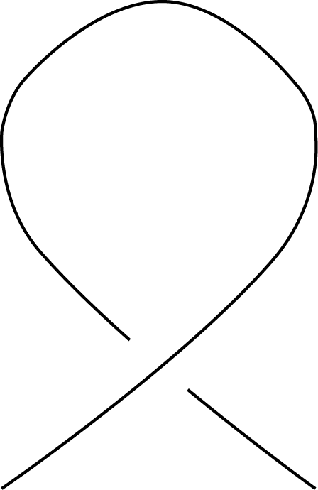
We will improve the latter bound for alternating links at a cost of introducing more parameters. Let us start by using Lackenby’s technique of modifying a link diagram through the addition of crossing circles. In particular, given a reduced alternating diagram of a link $K$, we encircle every twist that has at least four crossings by a simple closed curve, called a crossing circle. The obtained link $J$ is an augmented alternating link, and therefore is hyperbolic [Ada86]. Moreover, $S^{3}-K$ can be obtained from $S^{3}-J$ by Dehn fillings of the tori that correspond to crossing circles, and therefore the volumes satisfy $\mbox{\rm Vol}(S^{3}-K)\leq\mbox{\rm Vol}(S^{3}-J)$ by Theorem 6.5.6 in [Thu02] (the equality holds if and only if none of the twists is augmented, and the link is unchanged). Next we delete all crossings in the twists that we encircled, obtaining a new link $L$. The volume of $S^{3}-L$ is equal to the volume of $S^{3}-J$ by [Ada85]. Note that although the diagram of $J$ is not alternating, it is reduced in the sense that there are no loops as shown in Figure 1 (2).

Denote the diagram of $L$ by $D_{a}$ (subindex $a$ stands for “augmented”). Note that $D_{a}$ consists of 2-tangles (i.e. tangles from which there emerge four arcs pointing out) $T_{1},\ldots,T_{p}$, connected with each other or with itself through combinations of crossing circles (as, for example, in Figure 2 (1)). We may assume that none of $T_{k},\,k=1,\ldots p,$ is trivial in the sense of Lickorish [Lic81], i.e. none consists of two parallel strands only.

The diagram $D_{a}$ lies in the projection plane (denote the plane by $P$) except for small perturbations at crossings and the crossing circles. In [Men83], a technique of decomposing a link complement into two ideal polyhedra, one above $P$, and one below, is described. In particular, a constructive algorithm giving such a decomposition for alternating links is given. In the next few paragraphs, we somewhat recall and modify the technique.

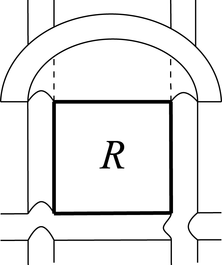
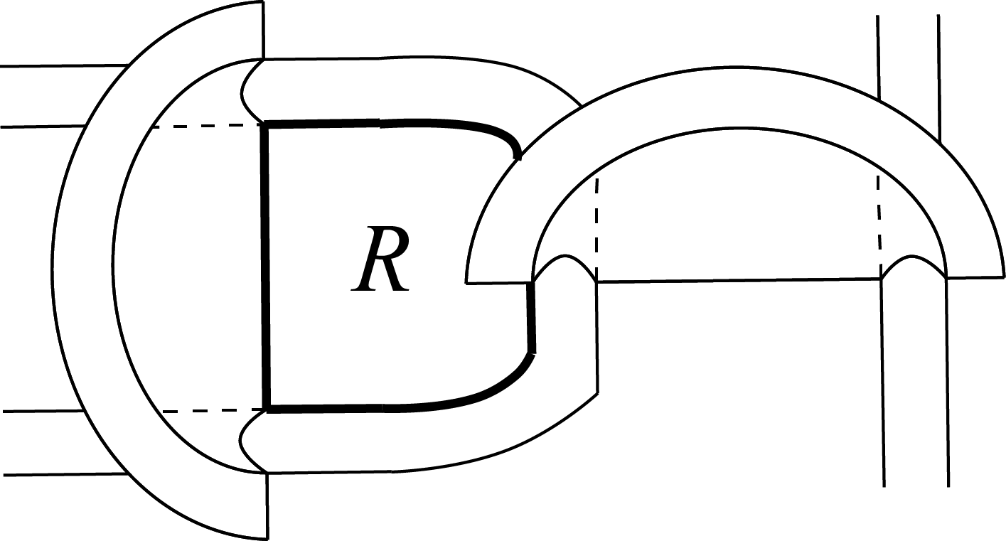
Imagine thickening the strands of $D_{a}$ until they (almost) touch each other at crossings. Each crossing circle pierces $P$ twice, and is divided into two half-circles by $P$. The two-punctured disk that it bounds (called a twisting disk) is divided by $P$ into two half-disks. The projection plane itself is divided into planar regions $R_{1},\ldots,R_{m}$ by thickened strands of a link and by the two-punctured disks that “cut” into it. More precisely, we say that a planar region $R_{j}$ is bounded by the segments in $P$ that lie either on the boundary of a thickened strand, or at the intersection of the interior of a two-punctured disk with $P$. A segment ends whenever it meets another strand, a crossing circle or a twisting disk. Figure 3 shows examples of a planar $4$-sided region and a planar $3$-sided region in the projection plane respectively.

Let us put two balls $B_{1}$ and $B_{2}$ in $S^{3}-L$, one above the projection plane, and one below. We inflate both balls simultaneously so that for an observer situated at the plane, the balls look like mirror images of each other. Eventually, the balls fill all of the $S^{3}-L$ and touch themselves and each other in the following way: (i) an upper ball touches itself at the upper half of every twisting disk; (ii) similarly, the lower ball touches itself at the lower half of every twisting disk; (iii) the upper ball touches the lower ball at every planar region $R_{j},\,j=1,\ldots,m,$ lying in the projection plane.

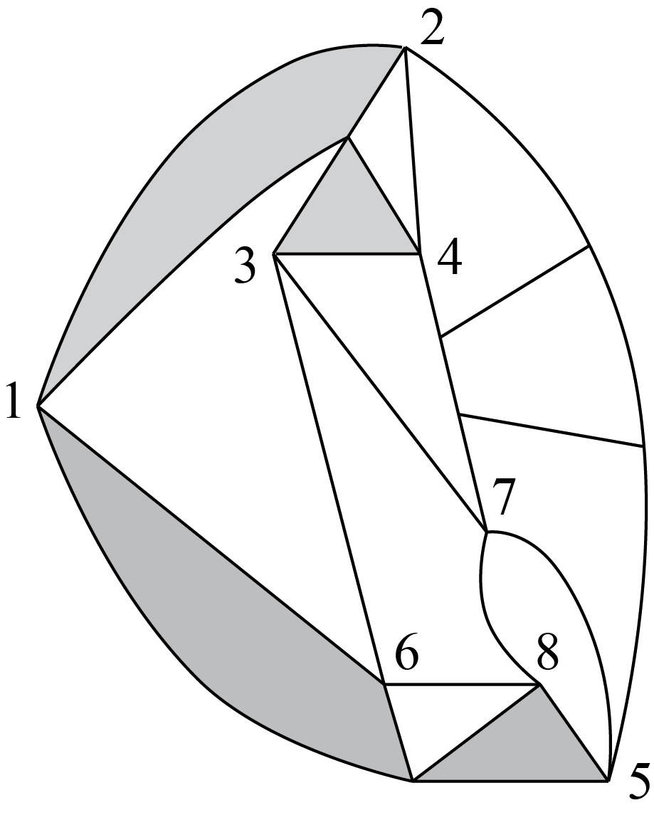
On the boundary of each $B_{i},i=1$ or $i=2$, there is a planar graph $\Gamma_{i}$ determined by the diagram $D_{a}$ as follows: Consider all parts of strands of the link that are visible from above of $P$. Subdivide them into segments $s_{1},s_{2},\ldots,s_{h}$ as described above. Each vertex of $\Gamma_{1}$ corresponds to one of $s_{i},\,i=1,2,\ldots,h$, and vice versa. The edges of $\Gamma_{1}$ arise where the thickened strands of $D_{a}$ “touch” each other, i.e. at crossings or crossing circles, in the following way. Where $B_{1}$ touches one of the half-disks from both sides, there are two regions in $\Gamma_{1}$, with three vertices each, connected by edges as a bow-tie, as in Figure 2 (2) (these faces are described in the appendix to [Lac04]). In addition, every crossing of $T_{k},\,k=1,2,\ldots p,$ yields four new edges of $\Gamma_{1}$. The four arcs in $S^{3}-L$, corresponding to these edges, travel from an overpass to an underpass of this crossing in $D_{a}$. The arcs are all homotopic to one another, as described in [Men83].

We have listed all edges and vertices of $\Gamma_{1}$ by now. Now two edges of $\Gamma_{1}$ meet at the same vertex if and only if the corresponding arcs in the link complement meet the same $s_{i}$. The construction implies that every vertex of the graph is now four-valent, with some multiple (to be precise, double) edges resulting from twists of $D_{a}$ that have at least four crossings. We will identify all the edges between the same two vertices $v_{1},v_{2}$, obtaining just one edge instead. The second graph, $\Gamma_{2}$, is constructed similarly, but using the segments of the strands of $D_{a}$ visible from below. Note that the diagram $D_{a}$ from above looks like the mirror image of the diagram from below, but with overcrossings and undercrossings interchanged.

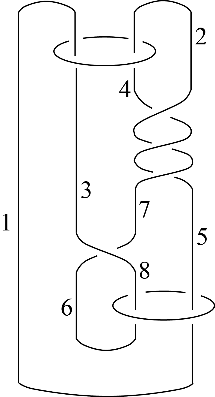
Figure 4 demonstrates an example of a link diagram (the leftmost picture) and the corresponding graph $\Gamma_{1}$ (the rightmost picture). Two pairs of the bow-tie faces are shaded in the graph, and all segments $s_{i}$ of $D_{a}$ are numbered, except for the two upper half-circles. On $\Gamma_{1}$, the numbering of the vertices corresponds to the numbering of $s_{i}$ in $D_{a}$.

The above description is somewhat implicit. To make it more instructional, we introduce an intermediate auxiliary picture.

As a first step, substitute all crossing circles in $D_{a}$ by bow-ties. Then substitute every crossing that is left by a 4-sided face, whose vertices lie on the edges of $D_{a}$ coming from this crossing (we will call such faces “pillowcases”). Whenever two vertices happen to be on one segment $s_{i}$ of $D_{a}$, merge them into one vertex. First we do this for the vertices of the pillowcase faces (we obtain a picture shown in Figure 4, in the middle, where edges of the new bow-tie and pillowcase faces are depicted by dotted lines, and the vertices shown as black dots). Then we perform merging for the rest of the vertices. We obtain the graph $\Gamma_{1}$ (Figure 4, right).

The balls $B_{1}$ and $B_{2}$ together with $\Gamma_{i}$ form polyhedra decomposing $S^{3}-L$. We will adopt the notation $P_{1}$ and $P_{2}$ for them. The link complement is obtained by folding the bow-ties in $P_{i}$ along each vertex to glue the pairs of triangles together; then folding each pillowcase so that two of its vertices that were on the same overpass are glued together; then, for each folded pillowcase located at a crossing (one pillowcase from $\Gamma_{1}$, and one from $\Gamma_{2}$), identifying the four edges (two from each pillowcase) as in [Men83]; then doubling along the rest of the faces. Figure 5 (1) illustrates what happens with a pillowcase in the process: its vertices are labeled by $a,b,c,d$. In particular, for the link diagram in Figure 4, in order to fold two pillowcases with vertices 3, 6, 7, 8 in $P_{1}$ and $P_{2}$, we first identify together 3 and 8 for $P_{1}$, and 6 and 7 for $P_{2}$. We then identify all four remaining pillowcase edges (two in $P_{1}$ and two in $P_{2}$) as in Menasco.

In the proof below, we will perform a triangulation of $S^{3}-L$, inspired by the one suggested by Ian Agol and Dylan Thurston in the appendix to [Lac04]. If every twist of $D$ has only one crossing, then the following theorem essentially recovers Adams’ Theorem 2.1 from [Ada83] (there is only a difference in the additive constant).

Note that our polyhedral decomposition is not the decomposition described by Menasco [Men83], since we introduced more vertices.

Let

be the colored Jones polynomial of an alternating link $K$, where $a_{n}$ and $\alpha_{n}$ are positive. The absolute values of the first three and last three coefficients of the colored Jones polynomial are independent of the color $n$ when $n\geq 3$ (see [DL06]), and $b_{n}$ and $\beta_{n}$ are independent of $n$ for $n\geq 2$. Moreover, the leading and trailing coefficients are known to satisfy $a_{n}=\alpha_{n}=1$ for all $n$.

We will use the values $b_{2},c_{2},c_{3},\beta_{2},\gamma_{2}$ and $\gamma_{3}$ to give a refinement of the Volumish Theorem [DL07, DL06] which states that for a prime, alternating, non-torus link $L$ the hyperbolic volume is bounded by:

where, as before, $v_{3}$ is the volume of a regular ideal hyperbolic tetrahedron.

The values $b_{2},c_{2},c_{3},\beta_{2},\gamma_{2}$ and $\gamma_{3}$ can be easily read off a reduced alternating diagram $D$ of an alternating link $L$ as follows. Suppose $D$ is twist reduced in the sense of [Lac04], i.e. the twist number $t(D)$ is minimized among all alternating diagrams of $L$. Color the diagram $D$ in black and white as a checkerboard in such a way that black regions are clockwise from an over-strand, while white regions are counter-clockwise from an over-strand; see Figure 7. One can associate a plane graph to the black regions by placing a vertex inside each black region, and by connecting two vertices if they are adjacent to the same crossing. We will call it the black checkerboard graph and denote it by $B(D)$. By using white regions instead, one obtains the planar white checkerboard graph $W(D)$. Note, that $B(D)$ and $W(D)$ are dual to each other. The vertices of $B(D)$ correspond to the faces of $W(D)$ and vice versa. The graphs $B(D)$ and $W(D)$ might have multiple edges between the same two vertices (such objects are often referred as multigraphs). If there are $m$ edges between two vertices $v_{1}$ and $v_{2}$ in a graph $G$, we leave just one of them (denote it by $e$) and delete the rest. The resulting graph is called the reduced graph, and we denote it by $G^{\prime}$. Using the initial graph $G$, we can assign multiplicity to every edge $e$ of $G^{\prime}$. Figure 8 shows a reduced alternating diagram of the knot $9_{20}$ together with its two reduced checkerboard graphs $B^{\prime}(D)$ and $W^{\prime}(D)$.

By $\tau_{B}$ or $\tau_{W}$ let us denote the number of triangles in $B^{\prime}(D)$ or $W^{\prime}(D)$. Finally, denote by $n_{B}(i)$ or $n_{W}(i)$ the number of edges of multiplicity at least $i$ in $B^{\prime}(D)$ or $W^{\prime}(D)$. Thus, by definition, $n_{B}(i)+n_{W}(i)=g_{i}$.

The following proposition follows immediately from results in [DL06]:

Combining Proposition 3.1 with Theorem 2.3 we obtain

The authors are grateful to Jessica Purcell for many enlightening conversations and interest in this work. We would also like to thank Colin Adams, Ian Agol, Dave Futer, Effie Kalfagianni, Marc Lackenby and Peter Shalen for helpful discussions on various occasions, and to the anonymous reviewer for aid in improving the paper. The authors acknowledge support from U.S. National Science Foundation grants DMS-1317942, DMS-0739382 (VIGRE), and DMS-1406588.

References

- [Ada83] Colin C. Adams, Hyperbolic Structures on Link Complements, Ph.D. thesis, University of Wisconsin, 1983.
- [Ada85] by same author, Thrice-Punctured Spheres in Hyperbolic 3-Manifolds, Trans. Amer. Math. Soc. 287 (1985), no. 2, 645–656.
- [Ada86] by same author, Augmented alternating link complements are hyperbolic, Low-dimensional topology and Kleinian groups (Coventry/Durham, 1984), London Math. Soc. Lecture Note Ser., vol. 112, Cambridge Univ. Press, Cambridge, 1986, pp. 115–130.
- [CR98] Patrick J. Callahan and Alan W. Reid, Hyperbolic Structures on Knot Complements, Chaos, Solitons and Fractals 9 (1998), no. 4/5, 705–738.
- [DL06] Oliver T. Dasbach and Xiao-Song Lin, On the head and the tail of the colored Jones polynomial, Compositio Mathematica 142 (2006), no. 05, 1332–1342.
- [DL07] by same author, A volumish theorem for the Jones polynomial of alternating knots, Pacific J. Math. 231 (2007), no. 2, 279–291.
- [FKP13] David Futer, Efstratia Kalfagianni, and Jessica S. Purcell, Guts of surfaces and the colored Jones polynomial, Lecture Notes in Mathematics, vol. 2069, Springer, Heidelberg, 2013.
- [Kas97] Rinat M. Kashaev, The hyperbolic volume of knots from the quantum dilogarithm, Letters in Mathematical Physics 39 (1997), no. 3, 269–275.
- [Lac04] Marc Lackenby, The volume of hyperbolic alternating link complements, Proceedings of the London Mathematical Society 88 (2004), no. 1, 204–224.
- [Lic81] W. B. Raymond Lickorish, Prime knots and tangles, Trans. Amer. Math. Soc. 267 (1981), no. 1, 321–332.
- [Men83] William Menasco, Polyhedra representation of link complements, Contemp. Math 20 (1983), 305–325.
- [MM01] Hitoshi Murakami and Jun Murakami, The colored Jones polynomials and the simplicial volume of a knot, Acta Mathematica 186 (2001), no. 1, 85–104.
- [Thu02] William P. Thurston, The Geometry and Topology of Three-Manifolds, electronic ed., 2002.
- [Tsv14] Anastasiia Tsvietkova, Exact volume of hyperbolic 2-bridge links, Comm. Anal. Geom. 22 (2014), no. 5, 881–896.
- [TT14] Morwen B. Thistlethwaite and Anastasiia Tsvietkova, An alternative approach to hyperbolic structures on link complements, Alg. Geom. Top. 3 (2014), 1307–1337.
- [Wee05] Jeffrey R. Weeks, Computation of Hyperbolic Structures in Knot Theory, Handbook of Knot Theory, Elsevier B. V., Amsterdam, 2005, pp. 461–480.
Oliver Dasbach
Department of Mathematics
Louisiana State University
Baton Rouge, Louisiana 70803, USA.
kasten@math.lsu.edu
Anastasiia Tsvietkova
University of California, Davis
One Shields Ave, Davis, CA 95616
tsvietkova@math.ucdavis.edu