Resilience of helical fields to turbulent diffusion II: direct numerical simulations

The purely resistive decay rate for the large scale magnetic energy $k_{1}=1$ mode is given by $2\eta k_{1}^{2}=4\times 10^{-4}$ (in dimensionless units) for runs A to D with $\eta=2\times 10^{-4}$. The slow decay regime for assessing the average decay rate is identified from $t=0$ to $t=t_{slow}$, where $t=t_{slow}$ is chosen as an arbitrary time comfortably less than the time, the curve evolves towards the transition region.

From the exponential fit to the initial slow decay regime, the average decay rate, $\gamma_{S}\sim 9\times 10^{-4}$, is almost twice the purely resistive decay rate for $k_{1}=1$ (where the large scale field resides). Nevertheless, this $\gamma_{S}$ is much smaller than the corresponding turbulent decay rate $\sim 2\eta_{t}k_{1}^{2}=(2/3){u_{rms}}/{k_{f}}$. For example, in the fiducial case of run B, where ${k_{f}}=5$ and with ${u_{rms}}=0.12$, we have $(2/3){u_{rms}}/{k_{f}}=0.016$, which is $\sim$ 18 times larger than the $\gamma_{S}$ obtained from DNS. Notice that the initial field is quite close to the equipartition strength. This goes to show that helical magnetic field of a sufficiently large inital strength, decays slowly at a rate which is of the order of the resistive time-scale and does not decay turbulently as one may have naively expected.

In the top panel of Fig. 6, we show the fit to LSHE evolution curve for runs A-D, using the form in Eq. 10. In the bottom panel of Fig. 6, we show the logarithmic slope of LSHE from the fit. On taking the mean of the logarithmic slope values in the resistive decay phase (from $t=0$ to $t=t_{slow}$), we again obtain the average estimate of $\gamma_{S}\sim 9\times 10^{-4}$. Hence matching with the $\gamma_{S}$ obtained from the first method.

Nonetheless, as can be seen from Fig. 6, the decay rate is continuously changing even in the slow decay phase. This slowly changing decay rate can be understood by considering the following.

The large scale field in the simulations is almost fully helical. Hence the large scale field is expected to decay according to the equations governing the evolution of magnetic helicity (which is a conserved quantity in the limit of $\eta\rightarrow 0$). For periodic or closed domains, evolution of the total magnetic helicity is given by,

All the quantities can be split into a mean (large scale) and a fluctuating (small scale) component. Accordingly, Eq. 11 can be written as,

where cross terms between the large and small scales vanish. Now, the small scale magnetic helicity is expected to reach steady state much faster than the large scale magnetic helicity. And hence, if $d\langle\overline{{\bf a}\cdot{\bf b}}\rangle/dt\rightarrow 0$ (as can be seen from Fig. 4), then large scale magnetic helicity decays at a rate decided by both $\langle{\overline{\bf J}}\cdot{\overline{\bf B}}\rangle$ and $\langle\overline{{\bf j}\cdot{\bf b}}\rangle$.

To obtain an equation for large scale helicity, one can use the mean field induction equation, given as,

where, ${\bf\mathcal{E}}=\overline{{\bf v}\times{\bf b}}$ is the electromotive force (or the EMF). Using the first order smoothing approximation (FOSA) (Moffatt, 1978; Krause & Raedler, 1980) or a $\tau$-approximation closure scheme (Pouquet et al., 1976; Blackman & Field, 2002; Rädler et al., 2003; Brandenburg & Subramanian, 2005), ${\bf\mathcal{E}}$ can be shown to be given by,

Here the kinetic alpha effect ($\alpha_{K}$), magnetic alpha effect ($\alpha_{M}$) and the turbulent diffusivity ($\eta_{t}$) are given by,

and $\tau$ is the correlation time which can be estimated to be of order the dynamical or eddy turn over time, $t_{eddy}=1/(u_{rms}k_{f})$. We uncurl Eq. 13 to obtain an equation for the mean vector potential, ${\overline{\bf A}}$. This can be used to obtain the dynamical equation for large scale helicity,

where we have put divergence terms to zero for periodic boundary conditions. The SSH evolution is obtained by subtracting Eq. 16 from Eq. 12,

From Eq. 16, we see that the large scale helical field would decay due to turbulent diffusion in the absence of the alpha effect. In our context of forced non-helical turbulence, the kinetic alpha effect is expected to be negligible. We verify this below, directly from DNS, in section 2.3. However, $\alpha_{M}$ could be generated by the action of turbulent diffusion on a large scale helical field. This can be seen explicity in the term, $\eta_{t}\langle{\overline{\bf J}}\cdot{\overline{\bf B}}\rangle$ in Eq. 17, which leads to the generation of $\langle\overline{{\bf a}\cdot{\bf b}}\rangle$ and hence $\langle\overline{{\bf j}\cdot{\bf b}}\rangle$ (even if were initially zero), having the same sign as $\langle{\overline{\bf J}}\cdot{\overline{\bf B}}\rangle$. Thus, the resulting $\alpha_{M}$ can in principle, balance the turbulent diffusion leading to a slow resistive decay of the LSHE. This implicitly constitutes large scale dynamo action, driven by the small scale current helicity.

We also see from Eq. 17, that $-\langle\alpha_{M}\cdot{\overline{\bf B}}^{2}\rangle\propto-{k_{f}}^{2}\langle\overline{{\bf a}\cdot{\bf b}}\rangle\langle{\overline{\bf B}^{2}}\rangle$, causes rapid damping of the SSH and leads to a steady state. For such a steady small scale helicity, Eq. 17 can be used to derive a relation between, $\langle{\overline{\bf J}}\cdot{\overline{\bf B}}\rangle$ and $\langle\overline{{\bf j}\cdot{\bf b}}\rangle$. We have for $d\langle\overline{{\bf a}\cdot{\bf b}}\rangle/dt\rightarrow 0$,

where, we have dropped the kinetic alpha term following Paper I. And by substituting the expression for $\alpha_{M}$ into Eq. 18, we have,

where, $M_{eq}$ is equal to $\rho u^{2}_{rms}/2$, in dimensionless units.

In the denominator of the RHS of the Eq. 19, if one considers that $\eta<<\eta_{t}$, and hence negligible, then with $\langle{\overline{\bf B}^{2}}\rangle/2M_{eq}=1$ (which is the case initially in the runs A-F), we have $\langle\overline{{\bf j}\cdot{\bf b}}\rangle\simeq\langle{\overline{\bf J}}\cdot{\overline{\bf B}}\rangle$. This implies that from Eq. 12, with $d\langle\overline{{\bf a}\cdot{\bf b}}\rangle/dt\rightarrow 0$, the LSHE decays at twice the resistive decay rate. This is an average estimate as ($\langle{\overline{\bf B}^{2}}\rangle/2$) is actually decaying slowly, and hence, $\langle\overline{{\bf j}\cdot{\bf b}}\rangle/\langle{\overline{\bf J}}\cdot{\overline{\bf B}}\rangle$ will increase over time, increasing the decay rate as can be seen from the bottom panel of Fig. 6. So, in fact the decay rate of LSHE is changing continuously even in the slow decay phase.

To further corroborate this continuous change in decay rate from theory, consider the following: Using the Eq. 19, we show in Fig. 7, an estimate of the quantity $M=\langle{\overline{\bf B}^{2}}\rangle/2M_{eq}=\langle\overline{{\bf j}\cdot{\bf b}}\rangle/\langle{\overline{\bf J}}\cdot{\overline{\bf B}}\rangle-{\eta}/{\eta_{t}}$, for run B as a solid yellow line. While LSHE calculated directly using Eq. 7 is shown in solid black. Then, we use the function in Eq. 10 to fit for both LSHE and $M$. Subsequently, we derive the logarithmic slope of the evolution curves using the fit and have shown them as black and yellow dash-dotted lines for direct LSHE and $M$, respectively. While the amplitude of the curve for $M$ is smaller than that of direct LSHE by $\sim 30\%$, the decay rate evolution predicted by $M$, matches closely with that of direct LSHE for most of the resistive decay phase. And we can see directly from Fig. 7, that decay rate is increasing constantly by a small amount for most of the slow decay phase. The match in the decay rate evolution of $M_{H}$ with that from the model $M$, shows that the two scale model is quite useful for understanding the simulation results in the slow decay phase.

Note that the Fig. 7 of Kemel et al. (2011), shows the decay of a highly superequipartition field with time. They find the initial decay rate for the magnetic energy to be $\gamma=-2\eta k^{2}_{1}$ (while we obtain the decay rate of $4\eta k^{2}_{1}$ for equipartition initial fields). For $\langle{\overline{\bf B}}^{2}\rangle/2>>M_{eq}$, from Eq. 19, $\langle\overline{{\bf j}\cdot{\bf b}}\rangle<<\langle{\overline{\bf J}}\cdot{\overline{\bf B}}\rangle$ and hence the large scale field is then predicted to decay at a purely resistive rate, which is consistent with their finding.

In passing we also note that the correct prediction of the rate of slow decay, $\gamma_{S}$ by the two scale model, which uses the closure relation for $\mathcal{E}$ in the Eq. 16, also lends some credence to such mean field closures.

We see from Fig. 4 that the LSHE decays at a much faster rate after it drops below some critical energy threshold. The fast decay phase is identified from some time after the curved transition region, to the time just before the field saturates, to a level determined by the tail of the fluctuation dynamo at large scales. (A more precise definition of the transition to the fast decay regime follows in section 3). Here the expected decay rate is the turbulent decay rate, $\gamma_{F}=2\eta_{t}k_{1}^{2}$, where $\eta_{t}=u_{rms}/3k_{f}$. In the simulations, ${u_{rms}}=0.12$ and $\eta_{t}=0.027$ for run A, $\eta_{t}=0.016$ for run B, $\eta_{t}=0.011$ for run C and $\eta_{t}=0.008$ for run D. The two scale model solutions match with expected decay rate of $2\eta_{t}k_{1}^{2}$ and are shown as the blue dashed lines in Fig. 4. It can be seen from Fig. 4, that in almost every DNS run, the slope of the LSHE curve in fast decay phase, is steeper than that of the two scale model solution. In fact, we find that the decay rate in the fast decay phase does not settle to a specific value, but keeps increasing with time, until the LS energy has decreased sufficiently to be dominated by noise.

The top panel of Fig. 6 shows that the fit for LSHE evolution curve does not reach an asymptotic slope at late times. The logarithmic slope of the large scale energy derived from the fit is shown in the bottom panel of Fig. 6 . It can be seen that for runs B-D, the logarithmic slope goes to values much larger than the turbulent decay rate. In all these cases, the large scale and small scale is constituted by a sharp split at $k=2$. However, this is an imperfect split and the effective large scale wave number, $k_{1}$ could increase to a higher value, as the large scale field decays. Such an increase in the wavenumber for ’large scale’ would then increase the expected turbulent rate.

Fig. 4 also shows SSH evolution obtained in the DNS with different ${k_{f}}$. Initially SSH is zero in the DNS, but rises to a non-zero value due to transfer of helicity from large to small scales and then stays roughly constant before decaying at late times. Paper I predicts the initial value for the steady state SSH, to be $(k_{1}/{k_{f}}^{2})M_{eq}$. The corresponding two scale solutions are shown as dashed lines in the Fig. 4, and we see that the steady SSH come close to expected values, but are larger in DNS runs B-F. This shows the limitations of the two scale model in capturing the whole spectral evolution of the DNS, nevertheless there is a reasonable agreement with expectations of the two model. Also, we find that the second slope of SSH, after the steady state phase, is steeper than the corresponding two scale model slope. Here again we expect that the effective wavenumber for small scale field increases from ${k_{f}}$ to larger values, resulting in a faster decay of SSH in the DNS. Whereas such an increase would be restricted in the two scale model, where the small scale is fixed at ${k_{f}}$.

Paper I has discussed at length, the contribution of kinetic alpha, $\alpha_{K}$ to $\mathcal{E}$. In the derivation leading to the two scale model, it was assumed the contribution of $\alpha_{K}$ to $\mathcal{E}$ is negligible as compared to $\alpha_{M}$. The kinetic alpha, $\alpha_{K}$, could be generated due to the Lorentz force and then would oppose the magnetic alpha, $\alpha_{M}$.

If $\alpha_{K}$ was significant, then the large scale helical field would decay much faster than the resistive decay rate. It was argued in Paper I that the generated $\alpha_{K}$ is indeed small. Nonetheless, it is important to make an estimate of $\alpha_{K}$ from the DNS and quantify its contribution to the net $\mathcal{E}$.

In Fig. 8, we show both $\alpha_{K}$ and $\alpha_{M}$ estimated from the DNS using Eq. 15. It can be seen that $\alpha_{K}$ fluctuates but is mostly negative and opposite in sign compared to $\alpha_{M}$ in the slow decay phase. One also sees from the Fig. 8, that $\alpha_{K}$ in the slow decay phase is found to be a factor of 4-5 smaller than $\alpha_{M}$ in the case of ${k_{f}}=5$ (Run B) and a factor of $\sim 10$ smaller in the case of ${k_{f}}=10$ (Run D). The contribution of $\alpha_{K}$ to the EMF is thus considerably smaller than $\alpha_{M}$ and hence subdominant as argued in Paper I. In the saturated phase, when all the magnetic helicity (and hence, $\alpha_{M}$) has decayed, the $\alpha_{K}$ alternates equally between being positive and negative values.

To identify this transition, we first consider the two scale model and then turn to the DNS. We solve numerically Eq. 16 and Eq. 17 of the two scale model, for different ${k_{f}}$, and then plot the time evolution of the large scale magnetic energy. To explore the behaviour of the transition point under the variations in ${k_{f}}$ alone, we keep $\mbox{R}_{M}$ and the initial magnetic energy, $M_{0}$ fixed across different numerical solutions. In the left hand side panel of Fig. 9, we show the decay of a fully helical large scale field with time for different ${k_{f}}=3,5,7,10,20$. The initial magnetic energy, $M_{0}=M_{eq}$ and the $\mbox{R}_{M}$ is fixed to a value of 120 which is comparable to the value in the DNS. One immediately notices that all the curves almost coincide. Note that in these solutions, the $\eta$ is the same, which explains the same slope in the slow decay regime. And in order to keep the turbulent decay rate, $\sim 2{u_{rms}}k_{1}^{2}/3{k_{f}}=2{u_{rms}}/3{k_{f}}$, the same, we compensate the increasing ${k_{f}}$, by increasing the ${u_{rms}}$. This forms the ideal experiment to understand the behaviour of the transition point as ${k_{f}}$ is varied. From the left panel of Fig. 9, the behaviour of the transition point is seen to be independent of the changing turbulent forcing scale, ${k_{f}}$.

To determine the transition point, we have adopted the following method. The evolving decay rate of the large scale helicity, from the two scale model is given by,

where, for fully helical fields, $\langle{\overline{\bf J}}\cdot{\overline{\bf B}}\rangle\sim k_{1}^{2}\langle{\overline{\bf A}}\cdot{\overline{\bf B}}\rangle$ and $\langle\overline{{\bf j}\cdot{\bf b}}\rangle\sim{k_{f}}^{2}\langle\overline{{\bf a}\cdot{\bf b}}\rangle$. Also, $\langle{\overline{\bf B}}^{2}\rangle\sim k_{1}\langle{\overline{\bf A}}\cdot{\overline{\bf B}}\rangle$ and therefore, Eq. 20 also describes the evolving decay rate of the large scale energy. The decay rate is expected to be fairly constant in the slow decay phase and sharply increases during the transition region and then settles to the turbulent decay value. Thus, the logarithmic slope of $\gamma$ will go through a maximum, when the decay rate changes the fastest. The point in time when the maximum occurs, can be then defined as the point of transition and the corresponding large scale energy is defined to be the transition energy. In the bottom right panel of Fig. 9, we show the $d(ln\gamma)/dt$ curves, while the top right panel shows the evolution of SSH. Note also that the maximum of $d(ln\gamma)/dt$ coincides with the point at which the SSH changes slope, i.e. SSH goes from nearly steady state value to decaying resistively at ${k_{f}}$. We thus find the transition energy to be $E_{c1}/M_{eq}=$0.031, 0.029, 0.026, 0.025, 0.025 for ${k_{f}}=$3, 5, 7, 10, 20 respectively. For completeness, along with the Eq. 20, we give here the corresponding equation for the small scale helical field,

In Fig. 10, we show similar plots of two scale solutions at a much larger $\mbox{R}_{M}=12000$, to also test the sensitivity of the results with respect to changes in $\mbox{R}_{M}$. The right panel of the Fig. 10, shows at the top, evolution of SSH while the bottom panel shows the evolution of $d(ln\gamma)/dt$. It can be seen from such plots for both the cases of $\mbox{R}_{M}$ = 120 and 12000, that as the ${k_{f}}$ increases, the point at which SSH changes slope, occurs later in time. And the corresponding large scale energy curve also transitions later in time. As a result, the transition energy would be similar across different ${k_{f}}$. The transition energy estimated in this case is $E_{c1}/M_{eq}=$ 0.0011, 0.0009, 0.0009, 0.0008 for $k_{f}=$ 5, 7, 10, 20 respectively. We find that the change in the transition energy from $\mbox{R}_{M}=120$ to $\mbox{R}_{M}=12000$ is by a factor of $\sim 25-30$. Thus interestingly, $E_{c1}$ seems to scale as $\mbox{R}_{M}^{-1/2}$.

Now we turn to the DNS and determine the transition energy of type $E_{c1}$ for the various runs in Table 1. In the case of simulations, we find that the decay rate in fast regime, is changing with time and and does not settle to a final value as is the case in the two scale model. Therefore, we do not find a maximum in the evolving logarithmic slope of LSHE to be able to determine the transition point. Instead, we adopt a slightly different method of estimating the transition energy in the case of DNS. From the right panels of Fig. 9 and Fig. 10, we pointed out that $d(ln\gamma)/dt$ is maximum when the SSH begins to decrease. Thus it seems plausible to define the transition point as the time when the SSH decreases from its initial steady state value by say, 50%. From Eq. 20, it can be seen that the first term on RHS goes to 0 when $\langle\overline{{\bf a}\cdot{\bf b}}\rangle=(k_{1}/{k_{f}}^{2})M_{eq}$ is in steady state, and by the time SSH, $\langle\overline{{\bf a}\cdot{\bf b}}\rangle$ decreases by 50%, the large scale field is expected to decay at a rate, of the order of the turbulent decay rate.

We use again the form in Eq. 10 to determine a fit for the SSH evolution. Then we estimate the point in time by when SSH decreases by 50% of its initial steady state value. The corresponding value of large scale energy is the transition energy. This method of determining the transition energy is conceptually similar to the one used for two scale model as it determines the point at which there is a change in the SSH evolution from steady state (or nearly zero decay rate) to a non-zero decay rate. This method of determining the transition energy is illustrated in the lower panels of Fig. 4 and Fig. 5. The vertical lines in these figures give the time when SSH has decreased by $50\%$ of its initial steady state value. This line intersects the LSHE curve at a transition energy value indicated by the horizontal line in each upper panel of Fig. 4 and Fig. 5. The transition energy thus determined, gives the critical energy as $E_{c1}\sim 0.034\ M_{eq}$ for run B. This is similar to the transition point we obtain from the corresponding two scale model solution of $E_{c1}\sim 0.029M_{eq}$. For the other runs A, C, D, E and F we find the transition energy to be $E_{c1}/M_{eq}=0.052,0.049,0.048,0.037$ and $0.034$ respectively, as can be read from the Fig. 4 and Fig. 5. This indicates the near universality of the transition point, $E_{c1}$, with respect to ${k_{f}}$ in a small range of $\mbox{R}_{M}$.

One can also determine the transition energy from the point of intersection between the slopes fit to the two decay regimes, slow and fast. The slope intersection method depends on accurate fits for the two decay regimes and hence is subject to uncertainity. Also, as we see in Fig. 6 that the slopes are not constant in any of the decay regimes, and are continually changing, and therefore, the determined slope is an approximate average estimate. The fit in especially the fast decay regime seems highly uncertain, depending on the window of time chosen. Hence we do not pursue this method for determining the transition energy.

Now we will examine the second kind of transition point, $E_{c2}$. This occurs when the initial magnetic field strength is lowered to a critical point below which the the field decays at a fast decay rate right from the beginning (i.e. the initial slow decay phase is now absent). We consider the evolution Eq. 16 for the large scale helicity and substitute $\langle\overline{{\bf j}\cdot{\bf b}}\rangle$ in $\alpha_{M}$ (in the emf $\mathcal{E}$ term) and $\langle{\overline{\bf J}}\cdot{\overline{\bf B}}\rangle$, with the corresponding two scale approximation of ${k_{f}}^{2}\langle\overline{{\bf a}\cdot{\bf b}}\rangle$ and $k_{1}^{2}\langle{\overline{\bf A}}\cdot{\overline{\bf B}}\rangle$, respectively. We then get,

Let us focus on the ideal limit of $\eta\rightarrow 0$, for which the total magnetic helicity is conserved at all times. Then, one can substitute for the small scale helicity in Eq. 22, $\langle\overline{{\bf a}\cdot{\bf b}}\rangle=\left(\langle\overline{{\bf A}\cdot{\bf B}}\rangle-\langle{\overline{\bf A}}\cdot{\overline{\bf B}}\rangle\right)$, where the total helicity $\left(\langle\overline{{\bf A}\cdot{\bf B}}\rangle\right)$ is conserved. Converting all the quantities to a dimensionless form, we get,

where $M_{1}=\langle{\overline{\bf B}}^{2}\rangle/(2M_{eq})=k_{1}\langle{\overline{\bf A}}\cdot{\overline{\bf B}}\rangle/(2M_{eq})$, $t/\tau=\tilde{t}$ and $M_{0}=M_{1}(\tilde{t}=0)$ is the normalised initial energy of the large scale helical field. Eq. 23 can now be solved to give,

When $M_{0}>(k_{1}/{k_{f}})^{2}$, at late times $\tilde{t}\to\infty$, we have,

indicating that, the reduction in the field strength is by a finite amount. When $M_{0}=(k_{1}/{k_{f}})^{2}$, Eq. 23 becomes $dM_{1}/dt=-(2/3)M_{1}^{2}$ and hence $M_{1}\rightarrow 0$ at late times.

And when $M_{0}<(k_{1}/{k_{f}})^{2}$, we obtain at late times when $\tilde{t}\to\infty$,

which implies that the large scale field undergoes a rapid decay. Hence, $(k_{1}/{k_{f}})^{2}$ forms a natural transition point, in the case of large $\mbox{R}_{M}$ (or here in the ideal limit of $\mbox{R}_{M}\rightarrow\infty$), which determines when the LSHE will directly transit to rapid decay. This was emphasized in Paper I but without giving the above argument. The question arises how well this threshold, which holds in the ideal limit, obtains for more realistic $\mbox{R}_{M}$, both in the two scale model and the DNS. We first reconsider the two scale model.

The left panel of Fig. 11, and Fig. 12, show the decay of fully helical large scale magnetic field for a set of decreasing initial field strengths for the two scale model. We have adopted ${k_{f}}=5$ (Fig. 11) and ${k_{f}}=20$ (Fig. 12), both with $\mbox{R}_{M}=12000$. While the inset in the left panels of Fig. 11 and Fig. 12 show the evolution of large scale energy with decreasing initial strengths, the main plots show the curves starting with subequipartition strength, time-shifted to maximally coincide the $M_{0}=1$ evolution. The labels in the plot indicate the value of $M_{0}$. The thick black curve is the case of $M_{0}=1$ (we will refer to this as the fiducial curve). In the curves beneath that of $M_{0}=1$, $M_{0}$ has been decreased to smaller and smaller values.

The right panel of Fig. 11 shows the evolution of the SSH. For stronger initial fields, SSH achieves a steady value and the resulting $\alpha_{M}$ is large enough to offset the turbulent diffusion. Then the large scale field decays initially at rate of the order resistive rate. When $M_{0}$ is below a critical value, the initial helicity in large scales is insufficient to generate a large enough small scale helicity, and $\alpha_{M}$, by turbulent diffusion. In this case the SSH decays, and the LSHE decays fast due to turbulent diffusion (uncompensated by the $\alpha_{M}$ effect).

It can be seen from the right panel of Fig. 11 that the dash-dotted blue line starting with $M_{0}=0.05$ is the last to reach a steady state indicating the presence of resistive decay regime initially. For such smaller $M_{0}\sim 0.04$ and below, the small scale helicity fails to rise to a steady state and subsequently decays indicating the absence of slow decay regime, which means that the large scale field directly starts decaying at a faster rate. This can be seen from the left panel of Fig. 11. Note that curves with $M_{0}$ above the threshold have sharp initial drop (as SSH builds up), but do not decrease in their energy significantly before joining the fiducial curve. On the other hand, the time-shifted purple dotted curve with $M_{0}=0.02$, which is below the threshold, drops by several orders of magnitude before joining the fiducial curve. Hence, we find that the transition point is close to the value of $(E_{c2}/M_{eq})=(k_{1}/{k_{f}})^{2}=0.04$ as expected from the work of Paper I and the Eq. 23 above.

Again the same exercise is repeated at ${k_{f}}=20$. In the Fig. 12, the solid green curve starting with $M_{0}=0.001$, which is below the expected critical energy of $(k_{1}/{k_{f}})^{2}$, is seen to drop in energy by few orders of magnitude before joining the fiducial curve. Hence in this case, we find the transition energy, $E_{c2}\sim 0.003\ M_{eq}$, as is seen from the Fig. 12. This value of $E_{c2}$ for the is again close to $(k_{1}/{k_{f}})^{2}M_{eq}$. Such large $\mbox{R}_{M}=12000$ is however beyond the scope of current DNS. Thus in the DNS studies below, where $\mbox{R}_{M}$ has a more modest value of $\sim 100$, we may not expect to see such a clear evidence of $E_{c2}$. Nevertheless, we do expect to check the consistency with the two scale model and hence indirectly substantiate the results of Paper I.

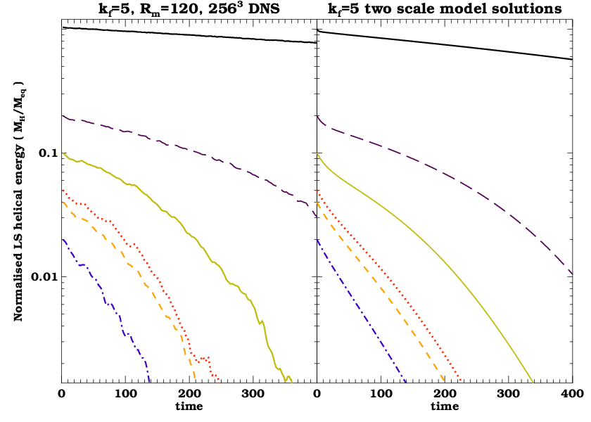
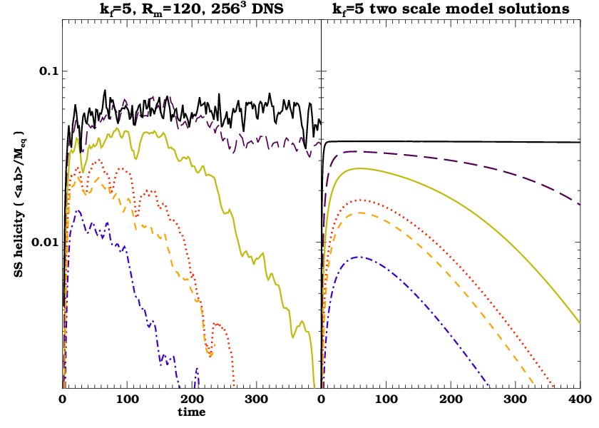
We have shown in Fig. 13, the results from the DNS runs G-K where the initial magnetic energy is lowered to smaller and smaller values compared to $M_{eq}$. In these set of simulations, we have fixed $k_{f}=5$, $u_{rms}\sim 0.12$ and $\eta=2\times 10^{-4}$, and thus $\mbox{R}_{M}=120$, while varying $M_{0}$. The top left panel of Fig. 13 shows the time evolution of large scale magnetic energy in the DNS, while the top right panel the results from the corresponding two scale model. The time evolution of the SSH in the DNS and corresponding two scale model are respectively shown in the bottom left and right panels of Fig. 13.

A comparison beween the DNS (left panel) and the 2-scale model (right panel) in Fig. 13, shows that there is a qualitative agreement between the two. For example, the slow decay rate of large scale energy of both are comparable, and so also are the amplitudes of the steady state small scale helicity. We also find that the average initial slopes (evaluated for the time period of t=0 to t=100) for all the runs G-K, listed in the Table 1, match closely with the estimate using Eq. 19, where the term in the denominatior, $\langle{\overline{\bf B}^{2}}\rangle/2{M_{eq}}$ is replaced with the value of $M_{0}$.

In Fig. 14, we show the fiducial curve where $M_{0}=1$ is the solid black line. We also show the evolution curves starting with sub-equipartition energies, time-shifted to lie on the fiducial curve. As pointed out earlier, a clear energy transition value would be revealed if curves with $M_{0}$ below the threshold decrease in their energy significantly before joining the fiducial curve. The graph shows all the curves nearly falling together without any such drop in the initial energy which at face value means no clear identification of $E_{c2}$ in the energy scale. However, from Eq. 19, it can be seen that the term $\eta/\eta_{t}=3/\mbox{R}_{M}$ has to be sufficiently small compared to $M_{0}$, to be able to discern the $E_{c2}$ dependence on ${k_{f}}$, for the subsequent evolution. If we compare the two terms in the denominator of Eq. 19, then we require, $3/\mbox{R}_{M}<<(k_{1}/{k_{f}})^{2}$. Otherwise, $\eta/\eta_{t}$ would become important before $M_{0}$ is lowered to $(k_{1}/{k_{f}})^{2}$, and one cannot discern the influence of ${k_{f}}$ on $E_{c2}$. With ${k_{f}}=5$ and $\mbox{R}_{M}=120$, $3/\mbox{R}_{M}=0.025$ and $(k_{1}/{k_{f}})^{2}=0.04$, thus the two terms are comparable. Hence, we seemingly need much higher $\mbox{R}_{M}$ runs ⁴⁴ 4 On the other hand, in the context of $E_{c1}$, it is the term $\eta/\eta_{t}$ which is responsible for the transition to faster decay phase. And we have seen that the transition energy $E_{c1}$ depends on $\mbox{R}_{M}$, scaling as $\mbox{R}_{M}^{-1/2}$ from the two scale model solutions. Thus DNS with even a modest $\mbox{R}_{M}$ can enable us to discern the transition energy, $E_{c1}$, which morover agrees reasonably with that predicted by the corresponding two scale model solutions. to be able to properly check the more conservative threshold of $E_{c2}/M_{eq}=(k_{1}/{k_{f}})^{2}$.

Note that in Fig. 13, as $M_{0}$ is decreased, approaching $E_{c2}$ from above, the subsequent decay seems to be at an increasingly higher rate. This can be understood from Eq. 19 (which applies only for $M_{0}>E_{c2}$ since only in that regime does $\langle\overline{{\bf j}\cdot{\bf b}}\rangle$ reach the steady state assumed by that equation.) For the curves with lower initial energy, the ratio, $\langle\overline{{\bf j}\cdot{\bf b}}\rangle/\langle{\overline{\bf J}}\cdot{\overline{\bf B}}\rangle$ will be larger, thus leading to a higher multiple of the resistive decay rate. This can be understood from examining Fig. 14. Since the curves with lower $M_{0}$, fall on the curve with $M_{0}=1$, later in time within the slow decay phase, they are expected to decay at an increasingly larger rate.

Overall we see a qualitative agreement between the DNS and the 2-scale model. This again indicates that the result of Paper I on the slow decay of helical magnetic fields which have $M_{0}>(k_{1}/k_{f})^{2}M_{eq}$, seems reasonably consistent with the simulations that we have performed so far. Though higher resolution simulations with high $\mbox{R}_{M}$ and small sub-equipartition initial fields are required to substantiate the above results.

In the distinct contexts of the previous two sections where we have identified the transition energies $E_{c1}$ and $E_{c2}$ we started with the SSH initially equal to zero. Here we discuss how the distinction between $E_{c1}$ and $E_{c2}$ can be traced to the distinct levels to which $\langle\overline{{\bf a}\cdot{\bf b}}\rangle$ builds up in the two cases.

The first context (section 3.1) in which we have identified the the transition energy is the fiducial case of $M_{0}=1$, for which we found a ${k_{f}}$ independent transition point $E_{c1}$. In this case, $\langle\overline{{\bf a}\cdot{\bf b}}\rangle$ builds up to a nearly steady state value during much of the resistive slow decay phase of $\langle{\overline{\bf A}}\cdot{\overline{\bf B}}\rangle$ before the fast decay occurs. In contrast, for the second context (section 3.2) of varying $M_{0}$, we found that when fast decay of the large scale field occurs right from the beginning, the helicity transferred from large scale to small scales never attains the aforementioned steady state value. The fast decay happens below a critical initial large scale helical energy value $E_{c2}$. If there is not enough initial helical large scale energy to supply the needed SSH, the large scale field decays fast. A source of SSH is crucial to explain the threshold of $E_{c2}$ on ${k_{f}}$ (Paper I).

To quantitatively study the importance of the role of SSH source in distinguishing $E_{c1}$ and $E_{c2}$, we can ask if setting the initial SSH equal to the maximum steady state value of the case of section 3.1 (rather than allow it to grow from zero) and then vary the initial $M_{0}$ (as in the case of section 3.2) do we recover $E_{c1}$?

Indeed, it is seen from Fig. 15, in the case of ${k_{f}}=5$, $\mbox{R}_{M}=12000$ and with the initial $\langle\overline{{\bf a}\cdot{\bf b}}\rangle=(k_{1}/{k_{f}}^{2})M_{eq}$, the two scale model solutions for varying $M_{0}$ fall together on the fiducial evolution curve for the context in section 3.1 For evolution starting at lower and lower energy values, the LSHE starts off initially with a flatter slope, but eventually joins the fiducial curve, which at that point in time is decaying at a much larger rate. The corresponding SSH quickly decays from the initial value of $(k_{1}/{k_{f}}^{2})M_{eq}$ to the value on the fiducial curve at that point in time. Additionally, it can be seen from Fig. 16 that if SSH is set to a value, $0<\langle\overline{{\bf a}\cdot{\bf b}}\rangle<(k_{1}/{k_{f}}^{2})M_{eq}$, then the two scale model solutions are similar to the second context, where SSH initially rises to attain the steady state value, and fails to do so when $M_{0}$ is at the threshold or below.

This shows that the difference between the two contexts that led to $E_{c1}\neq E_{c2}$ obtains due to the difference in the value of SSH attained in the early transient phase of the evolution.

References

- Beck (2012) Beck R., 2012, SSRv, 166, 215
- Bhat & Subramanian (2013) Bhat P., Subramanian K., 2013, MNRAS, 429, 2469
- Blackman & Brandenburg (2002) Blackman E. G., Brandenburg A., 2002, ApJ, 579, 359
- Blackman & Field (2002) Blackman E. G., Field G. B., 2002, Physical Review Letters, 89, 265007
- Blackman & Subramanian (2013) Blackman E. G., Subramanian K., 2013, MNRAS, 429, 1398 (Paper I)
- Brandenburg (2003) Brandenburg A., 2003, Computational aspects of astrophysical MHD and turbulence. p. 269
- Brandenburg (2011) Brandenburg A., 2011, Pramana, 77, 67
- Brandenburg & Subramanian (2005) Brandenburg A., Subramanian K., 2005, PhR, 417, 1
- Clarke (2004) Clarke T. E., 2004, Journal of Korean Astronomical Society, 37, 337
- Clarke et al. (2001) Clarke T. E., Kronberg P. P., Böhringer H., 2001, ApJ, 547, L111
- Field & Blackman (2002) Field G. B., Blackman E. G., 2002, ApJ, 572, 685
- Fletcher (2010) Fletcher A., 2010, in Kothes R., Landecker T. L., Willis A. G., eds, Astronomical Society of the Pacific Conference Series Vol. 438 of Astronomical Society of the Pacific Conference Series, Magnetic Fields in Nearby Galaxies. p. 197
- Govoni & Feretti (2004) Govoni F., Feretti L., 2004, International Journal of Modern Physics D, 13, 1549
- Haugen et al. (2004) Haugen N. E., Brandenburg A., Dobler W., 2004, PRE, 70, 016308
- Kazantsev (1967) Kazantsev A. P., 1967, JETP, 53, 1807
- Kemel et al. (2011) Kemel K., Brandenburg A., Ji H., 2011, PRE, 84, 056407
- Kleeorin et al. (2000) Kleeorin N., Moss D., Rogachevskii I., Sokoloff D., 2000, A&A, 361, L5
- Krause & Raedler (1980) Krause F., Raedler K. H., 1980, Mean-field magnetohydrodynamics and dynamo theory
- Moffatt (1978) Moffatt H. K., 1978, Magnetic field generation in electrically conducting fluids
- Pouquet et al. (1976) Pouquet A., Frisch U., Leorat J., 1976, Journal of Fluid Mechanics, 77, 321
- Rädler et al. (2003) Rädler K.-H., Kleeorin N., Rogachevskii I., 2003, Geophysical and Astrophysical Fluid Dynamics, 97, 249
- Ruzmaikin et al. (1988) Ruzmaikin A. A., Sokolov D. D., Shukurov A. M., eds, 1988, Magnetic fields of galaxies Vol. 133 of Astrophysics and Space Science Library
- Schekochihin et al. (2004) Schekochihin A. A., Cowley S. C., Taylor S. F., Maron J. L., McWilliams J. C., 2004, ApJ, 612, 276
- Subramanian (2002) Subramanian K., 2002, Bulletin of the Astronomical Society of India, 30, 715
- Vogt & Enßlin (2005) Vogt C., Enßlin T. A., 2005, A&A, 434, 67
- Yousef et al. (2003) Yousef T. A., Brandenburg A., Rüdiger G., 2003, A&A, 411, 321