A penalized likelihood approach for robust estimation of isoform expression
Abstract
Ultra high-throughput sequencing of transcriptomes (RNA-Seq) has enabled the accurate estimation of gene expression at individual isoform level. However, systematic biases introduced during the sequencing and mapping processes as well as incompleteness of the transcript annotation databases may cause the estimates of isoform abundances to be unreliable, and in some cases, highly inaccurate. This paper introduces a penalized likelihood approach to detect and correct for such biases in a robust manner. Our model extends those previously proposed by introducing bias parameters for reads. An L1 penalty is used for the selection of non-zero bias parameters. We introduce an efficient algorithm for model fitting and analyze the statistical properties of the proposed model. Our experimental studies on both simulated and real datasets suggest that the model has the potential to improve isoform-specific gene expression estimates and identify incompletely annotated gene models.
1 Introduction
In eukaryotes, a single gene can often produce more than one distinct transcript isoforms, through an important cell mechanism called alternative splicing. Alternative splicing can greatly enrich the diversity of eukaryote transcriptomes (Wang et al., 2008), especially in developmental and differentiation programs, and can contribute to disease when it is dysregulated (L¨®pez-Bigas et al., 2005). Study gene expression at specific transcript isoform level is therefore of great importance and interest to biologists.
Ultra high-throughput sequencing of transcriptomes (RNA-Seq) has enabled the accurate estimation of gene expression at individual isoform level (Wang et al., 2008). As of today, modern ultra high-throughput sequencing platforms can generate tens of millions of short sequencing reads from prepared RNA samples in less than a day. For these reasons, RNA-Seq has become the method of choice for assays of gene expression. To analyze increasing amounts of data generated from biological experiments, a number of statistical models and software tools have been developed (Jiang and Wong, 2009; Trapnell et al., 2010; Li and Dewey, 2011). For a review of the methods for transcript quantification using RNA-Seq, see Pachter (2011).
Although these methods have achieved great success in quantifying isoforms accurately, there are still many remaining challenging issues which may hinder their wider adoption and successful application by biologists. Systematic biases introduced during the sequencing and mapping processes (Li et al., 2010; Hansen et al., 2010; Roberts et al., 2011) as well as incompleteness of the transcript annotation databases (Pruitt et al., 2009; Hsu et al., 2006) can cause the estimates of isoform abundances to be unreliable. For example, recently, there have been periods of time where hundreds of new transcripts are discovered every month (Harrow et al., 2012), including occasional examples of thousands of new isoforms being identified in a single study, (Salzman et al., 2012; Salzman et al., 2013). These incomplete annotations can cause the estimates of isoform abundances to be unreliable (Black Pyrkosz et al., 2013).
This paper introduces a penalized likelihood approach to detect and correct for such biases in a robust manner. Bias parameters are introduced for read abundance, and an L1 penalty is used for the selection of non-zero bias parameters. We introduce an efficient algorithm for fitting this model and analyze its statistical properties. Our experimental studies on both simulated and real datasets show that transcript estimates can be highly sensitive to including or omitting parameters modeling read bias. Together, our results suggest that this method has the potential to improve isoform-specific gene expression estimates and improve annotation of existing gene models.
2 A penalized likelihood approach
2.1 The Model
We adopt the notation and extend the model in Salzman et al. (2011), which provides a flexible statistical framework for modeling for both single-end and paired-end RNA-Seq data, including insert length distributions. To state the model, for a gene with annotated distinct transcript isoforms, suppose the sequencing reads from are sampled from possible distinct read types. A read type refers to a group of reads (single-end or paired-end) with the same probability of being generated by sequencing a particular transcript (Salzman et al., 2011). We use to be the vector representing the abudance of the isoforms in the sample, to be the sampling rate matrix with its -th element denoting the rate that read type is sampled from isoform . Given and , we assume that the read count vector , where denotes the number of reads of type mapped to any of the isoforms, follows a Poisson distribution
The log-likelihood function is therefore
where the term was dropped because it does not contain .
In (Salzman et al., 2011), the sampling rate matrix is a set of parameters, assumed to be a known function of the sequencing library and gene. For single-end RNA-Seq data, the simplest model is to assume the uniform sampling model which assigns as where is the sequencing depth (proportional to total number of mapped reads) of the experiment if isoform can generate read type or assigns as otherwise. For paired-end RNA-Seq data, an insert length model can be used such that if read type can be mapped to isoform with insert length (fragment length) , where is the empirical probability mass based on all the mapped read pairs. Salzman et al. (2011) discuss these sampling rate models in more details.
Although these simplified sampling rate models usually work well in practice, there are systematic biases introduced during the sequencing and mapping processes which may caused biased estimates of the sampling rates and consequently biased estimates of isoform abundances. Several approaches have been developed to model and correct such biases (Li et al., 2010; Hansen et al., 2010; Roberts et al., 2011). However, completely removing sampling biases is almost impossible because modeling and identifying baiases in the technical procedure of sequencing and read mapping is often too complex. Including all possible transcript isoforms (de novo identification) also poses computational challenges and biases’; using all annotated transcripts in the model, many times exceeeding 10 per gene, can introduce non-identifyability of isoforms. However, while the vast majority of human genes have multiple annotated (and likely unannotated) transcripts, most cell types, or single cells, express only a subset of annotated transcripts.
To explore statistical modeling approaches that could improve transcript quantification with RNA-Seq, we present a flexible model to account for all different kinds of biases in estimated sampling rates. We assign a bias parameter to each read type and reparametrize as to constrain . When , there is no bias for read type . The actual effective sampling rate for read type from isoform now becomes , and the log-likelihood function is now
| (2.1) |
Since the number of observations is , which is smaller than the number of variables + in model (2.1), the model (2.1) is not identifiable. To solve this problem, we introduce a penalty on the bias parameters and formulate an L1-penalized log-likelihood
| (2.2) |
where is a tuning parameter.
Introducing the L1 penalty shrinks towards , consequently inflating compared to fitting a model with sparse but unbiased estimation of the parameters . One way to reduce such bias in the estimation of is to use a two-step approach for model fitting: first fit the model with the L1-penalized model, then fit the model without the L1 penalty, retaining only the non-zero ’s as model parameters. Clearly, to avoid nonidentifiable issues, the number of non-zero ’s must be smaller or equal than , which can be achieved by increasing the tuning parameter . The statistical properties of the two-step approach is discussed in Section 2.5.
Because (the number of distinct read types) is usually very large, especially for paired-end RNA-Seq data, we adopt the collapsing technique introduced in Salzman et al. (2011). We merge read types of proportional sampling rate vectors into read categories (which are minimal sufficient statistics of the model). This does not change the model (2.2) except that now represents a read category rather than a read type. Salzman et al. (2011) also introduced another data reduction technique which ignores all the read categories with zero read counts by introducing an additional term with the total sampling rates for each isoform . In this case, the log-likelihood function becomes
| (2.3) |
For simplicity, we will not discuss model (2.3) in this paper but our approach easily extends to deal with model (2.3).
2.2 Optimization
In this section we develop an efficient algorithm for fitting the model, i.e., maximizing the L1-penalized log-likelihood function (2.2) .
Proposition 2.1.
The L1-penalized log-likelihood function is biconcave.
Because is biconcave, we use Alternative Concave Search (ACS) to solve for and , by alternatively fixing one of them and optimize for the other. The sequence of function values generated by the ACS algorithm is monotonically increasing and is bounded from above (because it is a penalized log-likelihood function), conditions which guarentee convergence of the ACS algorithm.
Algorithm 2.2.
With fixed, can be solved with the following EM algorithm
| E-step: | ||||
| M-step: |
Alternatively, can be solved using the more efficient Newton-Raphson algorithm. In our implementation, we only execute one round of the EM iteration each time we optimize with fixed.
Proposition 2.3.
With fixed, has the following closed-form solution
| (2.4) |
where is the soft thresholding operator, where .
For more efficient convergence, we use an analytical property of values of and which maximize :
Proposition 2.4.
There is at least one set of and which maximize such that .
Accordingly, after each iteration which solves (2.4), our approach includes a step which centers the ’s around their median by updating as follows: .
2.3 Statistical Properties
Several statistical properties of the two-step approach introduced in Section 2.1 are provided in this section. First, we state an intuitive interpretation of the procedure:
Proposition 2.5.
Fitting the model using the two-step approach introduced in Section 2.1 is equivalent to fitting the model after removing all the observation ’s whose corresponding ’s are non-zero. In other words, the two model-fitting steps essentially perform outlier detection and removal, respectively.
This observation can be extended to prove that in the case of , the two-step procedure yields a consistent estimate of under the assumption that each . While may appear to be a trivial case, in fact, this approach is equivalent to considering a subset of the full model introduced in Salzman et al. (2011) where each read is considered if and only if it can be generated by exactly one isoform. Reasonable statistical power can be achieved with this approach, and it is of relatively wide use by biologists.
For convenience, the proposition and proof is stated for the case where , but this assumption can be relaxed to allow to be arbitrary. Also, from the proof, it is clear that larger choices of than also result in consistent estimates, but perhaps unnecessarily sparse models.
Proposition 2.6.
Under the assumptions that , for all , , the two-step approach yields a consistent estimator of .
3 Experiments
3.1 Simulations
In this section, we use simulation to study our model in various gene structures, relative isoform abundances, bias pattern throughout the gene and sequencing depths. For each simulation replicate, we estimate and using three approaches and compare their estimation accuracies. Throughout the simulations, we choose because of the consistency results we obtain with this choice.
- 1.
The conventional approach (Jiang and Wong, 2009; Salzman et al., 2011) with no bias correction (i.e., fix ).
- 2.
Our proposed one-step approach with bias correction (i.e., without doing the second step of estimation introduced in Section 2.1).
- 3.
Our proposed two-step approach with bias correction.
Example 3.1.
We first simulate the case that a gene has a single annotated isoform (i.e., ), read categories after collapsing (i.e., , e.g., the gene has exons). Suppose the estimate sampling rate matrix , where are the relative sampling rates for the five exons (e.g., each exon has the same length of 1000 bp), and is the relative sequencing depth (e.g., in Table 1 means there are 10M single end reads from the sequencing experiment. We assume and .
We simulate 100 replicates and report the average (and standard deviation) of estimation error of in L2 distance in Table 1. We also report the average (and standard deviation) of the number of ’s that are misidentified as zero vs. non-zero. Table 1 shows empirical results confirming our theory: if some , without bias correction, will not be estimated consistently. While both one-step and two-step approaches achieve consistent estimates of , the two-step approach is more efficient. On average, we misidentify less than one nonzero ’s.
| Seq Depth | No Bias | Bias (1-step) | Bias (2-step) | #Misientified |
|---|---|---|---|---|
| 10 | 1.32 (0.2) | 0.24 (0.14) | 0.13 (0.1) | 0.03 (0.17) |
| 100 | 1.26 (0.06) | 0.07 (0.04) | 0.04 (0.04) | 0.09 (0.29) |
| 1000 | 1.28 (0.02) | 0.02 (0.01) | 0.01 (0.01) | 0.05 (0.22) |
Example 3.2.
We now consider a case with , and , e.g., a gene with six exons and two isoforms differ by the inclusion/exclusion of the third exon. We assume and .
The simulation results for Example 3.2 are shown in Table 2. The performance of the three approaches is similar to that in Example 3.1.
| Seq Depth | No Bias | Bias (1-step) | Bias (2-step) | #Misientified |
|---|---|---|---|---|
| 10 | 3.78 (0.23) | 3.41 (1.85) | 3.02 (1.71) | 0.13 (0.34) |
| 100 | 3.76 (0.08) | 1.82 (1.28) | 1.4 (0.9) | 0.01 (0.1) |
| 1000 | 3.77 (0.03) | 0.45 (0.32) | 0.36 (0.26) | 0 (0) |
Example 3.3.
We now consider a case with , . For each replicate of the simulation, we randomly sample each element of as , where . We also randomly sample each element of and as and where .
The simulation results for Example 3.3 are shown in Table 3. The performance of the three approaches is similar to that in Examples 3.1 and 3.2. In particular, the approach without bias correction introduces huge estimation error in some of the cases (e.g., when is large and is small).
| Seq Depth | No Bias | Bias (1-step) | Bias (2-step) | #Misientified |
|---|---|---|---|---|
| 10 | 76.8 (471.72) | 1.22 (1.42) | 0.93 (0.69) | 2.17 (1.53) |
| 100 | 7792.35 (75161.75) | 2.56 (17.7) | 0.41 (0.41) | 2.2 (1.57) |
| 1000 | 406.35 (1934.52) | 0.42 (1) | 0.18 (0.41) | 2 (1.68) |
3.2 Real data analysis
We evaluted our model using real RNA-Seq data from the Gm12878 cell line generated by the ENCODE project (ENCODE Project Consortium et al., 2012). A total of single-end reads of 75 bp mapped to human chromosome 22 are used in the analysis. We use the human RefSeq annotation database (Pruitt et al., 2009) for our analysis. We ran both the conventional approach (without bias correction) and our proposed one-step approach (with bias correction) on this data set. 579 genes have estimated expression level using the unit RPKM (Mortazavi et al., 2008), and 65 of the 579 genes have at least 2-fold change in their gene expression estimates between the approaches with and without bias correction.
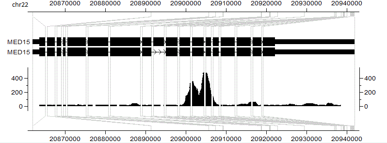
MED15 is an example of a gene with greater than 2-fold change in the total and expression of two isoforms of the gene with and without bias correction, shown in Figure 1. The center part of the gene has a much greater read density than the 5’ or 3’ ends. Without bias correction, MED15’s expression is estimated as 1487.11 RPKM (with the two isoforms estimated as 54.89 RPKM and 1432.22 RPKM, respectively). The one-step approach identifies this bias and down-weights the contribution of reads from center part of the gene to total gene expression. Consequently, it estimates the gene expression as 702.52 RPKM (with the two isoforms estimated as 53.65 RPKM and 648.87 RPKM, respectively).
The observed bias in MED15 could be due to mapping artifacts, or preferential amplification of portions of the gene during RNA-Seq library preparation. Further investigation, including experimental testing may be required to determine if either of these explanations for increased read density are explanatory. Another explanation could be that the gene model used for our model, which includes just two isoforms, is incomplete. For example, the observed increased read density could be due to expression of other isoforms of MED15 that include these regions.
4 Discussion
In this paper we choose , which seems to work reasonably well with both simulated and real data and which we have shown to produce consistent estimates of under reasonable assumptions. We believe that more research on statistical properites of different choices of may lead to improvement of our model in applied settings. For example, we plan to evaluate a standard approach of choosing by cross-validation, although it comes at the cost of more intensive computation. Also, as our proof of consistency shows, choosing values of larger than will also yield consistent estimators of under the regime analyzed in Proposition 2.6.
From (2.4), it is apparent that the larger the value of , the relatively smaller portion of it is affected by . Intuitively, the proposed approach works the best when the read categories are of similar sizes. In our real data experiment, we collapsed reads into exons and junctions to roughly fulfill this condition, and simulation demonstrates that our proposed approach is not very sensitive to how collapsing is performed. An alternative approach is to use as the weight for the corresponding , i.e., by letting . All the statistical properties and optimization techniques introduced in the paper can be adapted to this new penalty function with only minor modifications. In simulations (results not shown here), this new penalty function does not perform noticeably better than the current penalty function. There may be advantages and disadvantages to increasing penalties for biases corresponding to larger .
Although the two-step approach appears to be slightly more efficient than the one-step approach in our simulations, it has several critical drawbacks: 1) It requires an increase in computation up to a factor of two; 2) It may introduce non-identifiable issue in the second step of estimation when the number of nonzero ’s identified in the first step of estimation is large; and 3) It makes parameter estimates sensitive to . Therefore, we use the one-step approach in our real data experiment and we plan to study the two-step approach in more details in future work.
The example of MED15 highlights another use of fitting bias parameters. First, in the presence of unannotated isoforms of a gene, correcting for bias in read sampling may be correcting for real biological confounding. In such scenarios, simulation suggests that correcting for bias improves model fit and quantification conditional on the gene models used for the study. For example, the two transcripts of MED15 in Figure 1 are probably more realistically estimated by our bias-corrected model. In addition, screening genes with large estimated bias parameters may be a tool for identifying unannotated transcripts or incomplete models used in the mapping step.
Finally, the approach introduced in this paper is adapted and stated for the isoform expression estimation problem, which is formally a Poisson regression model with identity link function. We believe it may be possible to generalize it to other generalized linear models such as linear regression models and logistic regression models, for which other practical applications may exist as well.
Appendix
Proof of Proposition 2.1.
where and are concave, is concave because is concave and is concave and non-decreasing, and is biconcave because both and are convex. ∎
Proof of Proposition 2.3.
Fixing , since the L1-penalty is decomposable, can be written as the sum of terms , where
Therefore, . Note the second term of does not contain . Since is non-differentiable, we take the subdifferential of at
where if and if . It can be verified that (2.4) is the solution to the equation . ∎
Proof of Proposition 2.4.
Suppose and are such that . Let and , where , then
∎
Proof of Proposition 2.5.
Without log of generality, suppose and after the first step of model fitting with the L1 penalty. In the second step of model fitting without the L1 penalty, we have , where
| (4.1) |
Solving
we have
| (4.2) |
Plugging (4.2) into (4.1), we have
therefore where
is exactly the log-likelihood after removing all the observation ’s whose corresponding ’s are non-zero. ∎
Proof of consistency
In this section, we assume for convenience and prove Proposition 2.6, that is, the two-step estimation procedure is consistent, in several steps.
Proposition 4.1.
For , any solution that maximizes under the constraint that for must be a fixed point of the E-M algorithm and therefore, plugging in to Equation implies that if ,
| (4.3) |
Therefore, on the event for some a subset of where A is defined by if and only if , the penalized log-likelihood reduces to:
| (4.4) |
Proof of 4.1.
The proof is by contradiction: if the solution does not maximize these equations, iterating 1 step of the E or M will increase the likelihood. Plugging in the solution for in terms of as in the proof of . ∎
Proposition 4.2 (Corollary of Proposition 2.4).
Under the constraint for all , the solution maximizing the likelihood (2.2) must estimate at least one .
Suppose is where is the “sequencing depth” and does not depend on , and and
Limit results are stated for the case where . In model (2.2), assume the are non-decreasing in . Note that exists by Prop. 4.2.
Proposition 4.3.
Consider the model in (2.2) under a further assumption that for some fixed where , for all and for all . The maximum likelihood estimator takes the form
where indexes the subset of estimated to be zero, and takes the form for all .
Proposition 4.4.
If a.s., where is the indicator function, on this event, a.s.
Proof of Prop. 4.4.
The first part is proved below. From the above equation 4.4, it is clear that a.s. implies a.s. ∎
Define the following procedure with tuning parameter and the order statistics of observed counts : Intuitively, Equation 4.4 together with the closed form solution for in terms of an estimate of show that a fixed point of the EM algorithm will define the set of variables with non-zero as those where, omitting them, the estimate of plus is less than any observed ommitted.
To see this formally, for each , let . Define as the smallest index such that . If no such exists, define .
Proposition 4.5.
Suppose for some fixed where , for all and for all , i.e., and Fix . Then, as , a.s.
Proof.
Fix where and , ie. corresponds to a and corresponds to a . The CLT implies a.s. as .
Therefore, summing over all and satisfying ,
It follows that for any and with and ,
and hence that for any constant not growing with ,
- 1.
For all ,
and
- 2.
For all (in particular, for )
which implies that
Therefore,
That is,
which implies
∎
Acknowledgements
HJ’s research was supported in part by an NIH grant 5U54CA163059-02 and a GAPPS Grant from the Bill & Melinda Gates Foundation. JS was supported by NIH grant 1K99CA16898701 from the NCI.
References
- Black Pyrkosz et al. (2013) A. Black Pyrkosz, H. Cheng, and C. Titus Brown. RNA-Seq Mapping Errors When Using Incomplete Reference Transcriptomes of Vertebrates. ArXiv e-prints, Mar. 2013.
- ENCODE Project Consortium et al. (2012) ENCODE Project Consortium, B. E. Bernstein, E. Birney, I. Dunham, E. D. Green, C. Gunter, and M. Snyder. An integrated encyclopedia of DNA elements in the human genome. Nature, 489(7414):57–74, Sept. 2012. ISSN 1476-4687.
- Hansen et al. (2010) K. D. Hansen, S. E. Brenner, and S. Dudoit. Biases in illumina transcriptome sequencing caused by random hexamer priming. Nucleic Acids Res, 38(12):e131, Jul 2010.
- Harrow et al. (2012) J. Harrow, A. Frankish, J. M. Gonzalez, E. Tapanari, M. Diekhans, F. Kokocinski, B. L. Aken, D. Barrell, A. Zadissa, S. Searle, I. Barnes, A. Bignell, V. Boychenko, T. Hunt, M. Kay, G. Mukherjee, J. Rajan, G. Despacio-Reyes, G. Saunders, C. Steward, R. Harte, M. Lin, C. Howald, A. Tanzer, T. Derrien, J. Chrast, N. Walters, S. Balasubramanian, B. Pei, M. Tress, J. M. Rodriguez, I. Ezkurdia, J. van Baren, M. Brent, D. Haussler, M. Kellis, A. Valencia, A. Reymond, M. Gerstein, R. Guig¨®, and T. J. Hubbard. Gencode: the reference human genome annotation for the encode project. Genome Res, 22(9):1760–1774, Sep 2012.
- Hsu et al. (2006) F. Hsu, W. J. Kent, H. Clawson, R. M. Kuhn, M. Diekhans, and D. Haussler. The ucsc known genes. Bioinformatics, 22(9):1036–1046, May 2006.
- Jiang and Wong (2009) H. Jiang and W. H. Wong. Statistical inferences for isoform expression in rna-seq. Bioinformatics, 25(8):1026–1032, Apr 2009.
- Jiang et al. (2010) H. Jiang, F. Wang, N. P. Dyer, and W. H. Wong. Cisgenome browser: a flexible tool for genomic data visualization. Bioinformatics, 26(14):1781–1782, Jul 2010.
- Li and Dewey (2011) B. Li and C. N. Dewey. Rsem: accurate transcript quantification from rna-seq data with or without a reference genome. BMC Bioinformatics, 12:323, 2011.
- Li et al. (2010) J. Li, H. Jiang, and W. H. Wong. Modeling non-uniformity in short-read rates in rna-seq data. Genome Biol, 11(5):R50, 2010.
- L¨®pez-Bigas et al. (2005) N. L¨®pez-Bigas, B. Audit, C. Ouzounis, G. Parra, and R. Guig¨®. Are splicing mutations the most frequent cause of hereditary disease? FEBS Lett, 579(9):1900–1903, Mar 2005.
- Mortazavi et al. (2008) A. Mortazavi, B. A. Williams, K. McCue, L. Schaeffer, and B. Wold. Mapping and quantifying mammalian transcriptomes by rna-seq. Nat Methods, 5(7):621–628, Jul 2008.
- Pachter (2011) L. Pachter. Models for transcript quantification from RNA-Seq. ArXiv e-prints, Apr. 2011.
- Pruitt et al. (2009) K. D. Pruitt, T. Tatusova, W. Klimke, and D. R. Maglott. Ncbi reference sequences: current status, policy and new initiatives. Nucleic Acids Res, 37(Database issue):D32–D36, Jan 2009.
- Roberts et al. (2011) A. Roberts, C. Trapnell, J. Donaghey, J. L. Rinn, and L. Pachter. Improving rna-seq expression estimates by correcting for fragment bias. Genome Biol, 12(3):R22, 2011.
- Salzman et al. (2011) J. Salzman, H. Jiang, and W. H. Wong. Statistical modeling of rna-seq data. Statistical Science, 26(1):62–83, 2011.
- Salzman et al. (2012) J. Salzman, C. Gawad, P. L. Wang, N. Lacayo, and P. O. Brown. Circular rnas are the predominant transcript isoform from hundreds of human genes in diverse cell types. PLoS ONE, 7(2):e30733, 02 2012.
- Salzman et al. (2013) J. Salzman, R. E. Chen, M. N. Olsen, P. L. Wang, and P. O. Brown. Cell-type specific features of circular rna expression. PLoS Genet, 9(9):e1003777, 09 2013.
- Trapnell et al. (2010) C. Trapnell, B. A. Williams, G. Pertea, A. Mortazavi, G. Kwan, M. J. van Baren, S. L. Salzberg, B. J. Wold, and L. Pachter. Transcript assembly and quantification by rna-seq reveals unannotated transcripts and isoform switching during cell differentiation. Nat Biotechnol, 28(5):511–515, May 2010.
- Wang et al. (2008) E. T. Wang, R. Sandberg, S. Luo, I. Khrebtukova, L. Zhang, C. Mayr, S. F. Kingsmore, G. P. Schroth, and C. B. Burge. Alternative isoform regulation in human tissue transcriptomes. Nature, 456(7221):470–476, Nov 2008.