HOW EMPTY ARE DISK GAPS OPENED BY GIANT PLANETS?
Abstract
Gap clearing by giant planets has been proposed to explain the optically thin cavities observed in many protoplanetary disks. How much material remains in the gap determines not only how detectable young planets are in their birth environments, but also how strong co-rotation torques are, which impacts how planets can survive fast orbital migration. We determine numerically how the average surface density inside the gap, , depends on planet-to-star mass ratio , Shakura-Sunyaev viscosity parameter , and disk height-to-radius aspect ratio . Our results are derived from our new GPU-accelerated Lagrangian hydrodynamical code PEnGUIn, and are verified by independent simulations with ZEUS90. For Jupiter-like planets, we find , and for near brown dwarf masses, . Surface density contrasts inside and outside gaps can be as large as , even when the planet does not accrete. We derive a simple analytic scaling, , that compares reasonably well to empirical results, especially at low Neptune-like masses, and use discrepancies to highlight areas for progress.
Subject headings
accretion, accretion disks — methods: numerical — planets and satellites: formation — protoplanetary disks — planet-disk interactionsI. INTRODUCTION
Observational studies of giant planet formation will begin in earnest once we detect planets still embedded in their natal gas disks. Directly imaging young gas giants is made easier by their ability to clear material away from their orbits. Planetary (Lindblad) torques open gaps while viscous torques fill them back in [1]: a balance between these torques sets the equilibrium surface density near the planet. There are hints of gap clearing by planets in so-called “transitional” disks having optically thin cavities [2, 3, 4, e.g.,]. Transition disk holes are surprisingly large; one gap opened by a single planet would be too narrow to explain the observed cavity sizes that range up to 100 AU, and so a given system might have to contain multiple super-Jovian planets to clear a wide enough swath [5, 6, e.g.,]. Even so, the holes are so optically thin that planets alone seem incapable of torquing material strongly enough to compete with viscous diffusion — at least for typically assumed parameters — and appeals are made to opacity reductions through grain growth or dust filtration at the outer gap edge [7, 8]. Part of the motivation of our study is to expand the parameter space explored and see how empty a gap can be cleared.
Determining gap surface densities and corresponding optical depths is relevant not only for observations but also for theory: material that co-rotates with the planet (executing quasi-horseshoe orbits) can backreact gravitationally on the planet and influence its dynamical evolution. The co-rotation torque takes its place among the litany of resonant planet-disk interactions that can alter orbital eccentricities and semimajor axes (for a review, see Kley and Nelson 9). The delicate balance of forces within the gap, including the thermodynamic behavior of matter there, may determine how low-mass and giant planets survive the threats of Types I and II orbital migration (Ward 10; see also section 2.2 of Kley and Nelson 9 and references therein).
Despite its importance, --- the surface density averaged over the bottom of the gap --- remains poorly understood. Notwithstanding the huge number of simulations of planet-disk interactions published in the past two decades,11 1 Much of the literature is marked by a peculiar insistence on plotting surface density on a linear scale. The practice is unhelpful since surface density contrasts in and out of gaps can span orders of magnitude — indeed they must if they are to reproduce the enormous optical depth contrasts inferred from observations of transition disks (e.g., Dong et al. 8). a systematic parameter study has yet to be performed that determines as a function of planet-to-star mass ratio ; Shakura-Sunyaev viscosity parameter ; and disk height-to-radius aspect ratio (equivalently, disk temperature) . Crida et al. [11] examined how these parameters influence gap shape and width, but not gap depth — i.e., they studied the onset of the gap, but not the bottom of the gap. The numerics can be challenging. Measuring accurately requires global simulations that (i) resolve the disk well in at least azimuth and radius ; (ii) resolve large density contrasts; (iii) converge with time to a steady state; (iv) model how the planet accretes from the ambient flow; and (v) possess well-separated radial boundaries that maintain a steady mass accretion rate across the entire domain, i.e., the simulation presumably should enforce constant , as befits real accretion disks. Feature (v) is captured by only a minority of studies, and feature (iv) can only be mocked up in a parameterized way [12, 5, e.g.,].
This paper aims to provide an empirical relation for for a single non-accreting giant planet on a fixed circular orbit embedded in a 2D, locally isothermal, steadily accreting disk. We restrict our study to disk gas only, and ignore how dust and gas flows might differ. We utilize two independent codes: ZEUS3D [13], and PEnGUIn, a new Lagrangian PPM (piecewise parabolic method)-based code that we have implemented on multiple GPUs (graphics processing units). To the extent possible, results from one code will be validated against the other.
I.1. An Analytic Scaling Relation
Although our study is primarily numerical, we derive here an approximate analytic relation for that we will use to put our numerical results in context. We admit at the outset that our derivation can hardly be called such, as our reasoning will ignore many details and make assumptions not carefully justified. But as the rest of our paper will show, the simple relation we now present will yield results surprisingly close to those of detailed numerical simulations.
First examine the outer disk, exterior to the planet’s orbit. The outer Lindblad torque exerted by the planet transmits angular momentum outward at a rate:
| (1) |
where is the disk angular frequency [1]. This is the total torque from linear perturbations to one side of the planet, integrated over all resonances up to the torque cut-off at azimuthal wavenumber (see, e.g., equation 2 of Crida et al. 11, and references therein). Note that we have used , the surface density averaged over the bottom of the gap, in our evaluation of the integrated Lindblad torque. Our justification for this choice is that the integrated torque is dominated by resonances at the torque cut-off, i.e., at distances from the planet (see figures 2 and 3 of Goldreich and Tremaine 1), and bottoms of gaps opened by giant planets in gas disks typically extend this far (see, e.g., the simulated gaps of Crida et al. 11, or our Figure 2). One caveat is that the linear theory from which equation (1) originates is formally valid only for low-mass planets for which ; the highest-mass planets we simulate will violate this condition, and indeed for such super-Jovian objects our numerical simulations will reveal deviations from the simple-minded scaling law we derive in this section.
In steady state, the outward transmission of angular momentum by the (outer) Lindblad torque must be balanced by the angular momentum transmitted inward by the viscous torque:22 2 There is also a so-called “pressure” torque of comparable magnitude to the Lindblad and viscous torques [11], but we neglect this third torque for our order-of-magnitude derivation.
| (2) |
where is the kinematic viscosity [14, e.g.,]. Here we have used , the surface density at the gap periphery — or more conveniently, the surface density at the planet’s location if the planet were massless — to evaluate . The viscous torque depends on the gradient of , and this gradient is larger outside the flat-bottomed gap than inside it (see, e.g., the gap profile shown in Figure 2; by “gap periphery” we mean a location like , where the gradient might reasonably be approximated as , which is what equation 2 essentially assumes). Conscripting in this way is a gross simplification, but alternatives would require that we actually compute the precise shape of the gap, which is what we are trying to avoid with our order-of-magnitude derivation.
Usually one thinks of viscous torques as transmitting angular momentum outward, but in the gap edge of the outer disk, the direction of viscous transport is inward because the surface density there has a sharp and positive gradient ().
Setting yields
| (3) |
Exactly the same scaling relation applies to the inner disk, interior to the planet’s orbit. The signs in the inner disk are reversed from those in the outer disk: the inner Lindblad torque transmits angular momentum inward, while the local viscous torque transmits angular momentum outward.
As we were completing our numerical tests of equation (3) and preparing our manuscript for publication, we became aware of the study by Duffell and MacFadyen [15] who found the same scaling relation on purely empirical grounds (although these authors did not explicitly vary the Mach number ). Duffell and MacFadyen [15] concentrated on the low-mass regime. Our study complements theirs by studying the high-mass regime; we will see to what extent equation (3) also holds true for giant planets. See also our §IV.3 where we discuss to what extent the short derivation given in this subsection captures the whole story.
I.2. Plan of This Paper
Section II contains our numerical methods and simulation parameters. Section 3 presents our results for . Section 4 concludes and charts directions for future work.
II. NUMERICAL METHODS
We numerically simulate a planet on a fixed circular orbit embedded in a co-planar, viscously accreting disk. Our two independent codes, PEnGUIn and ZEUS3D, solve the usual mass and momentum equations in two dimensions; we give here the equations in the inertial, barycentric frame (although neither code actually works in this frame; see §II.1 and §II.2 for the technical details):
| (4) |
| (5) |
where is the Lagrangian derivative, is the surface density, is the vertically integrated pressure, is the velocity, is the Newtonian viscous stress tensor, and is the gravitational potential of the central star and planet (but not the disk). In polar coordinates, ; in component form, equation (5) reads:
| (6) | ||||
| (7) |
Here is the kinematic viscosity following Shakura and Sunyaev [16], with equal to the sound speed. We complete the equation set with a locally isothermal equation of state , with so that the disk aspect ratio constant.
In the center-of-mass frame,
| (8) |
where and are the masses of the star and the planet, respectively; and are their radial positions, with the total (fixed) separation; and are their angular positions; and is the smoothing (a.k.a. softening) length of the planet’s potential. We set and so that the planet’s orbital frequency and period .
II.1. PEnGUIn: Code Description
PEnGUIn (Piecewise Parabolic Hydro-code Enhanced with Graphics Processing Unit Implementation) is a Lagrangian, dimensionally-split, shock-capturing hydrodynamics code. We defer a detailed description to a future paper, and here just mention a few salient points. The code is written in CUDA-c and runs on multiple GPUs (graphics processing units) for accelerated performance. It uses the piecewise parabolic method (PPM; Colella and Woodward 17), and its main solver is modelled after VH-1 [18] with two main differences: (i) PEnGUIn explicitly conserves angular momentum by replacing, as one of the quantities a fluid element carries in the Lagrangian frame, the angular speed with the specific angular momentum, and (ii) PEnGUIn uses a non-iterative Riemann solver for isothermal flows; see Balsara [19], and note that their Lagrangian re-map formulation applies not only to strictly isothermal flows, but also to locally isothermal flows under the two-shock approximation by allowing for different sound speeds for left- and right-moving waves. PEnGUIn also contains a module that computes the divergence of the stress tensor through piecewise parabolic interpolations.
Technically, PEnGUIn’s reference frame is a barycentric frame that rotates at ; thus the planet’s position is fixed in time, but the Coriolis force is not computed as an explicit source term. Rather, it is absorbed into the conservative form of the angular momentum equation [20].
GPU-acceleration is optimal for programs that are massively parallel; PEnGUIn achieves parallelization through memory management and domain splitting. The hardware used for this paper are three GTX-Titan graphics cards all connected to a single node. Running in double precision on all three cards simultaneously, PEnGUIn takes 12 seconds to run per planetary orbit for .
II.2. ZEUS90: Code Description
For comparison with PEnGUIn, we also carried out simulations with ZEUS90: a modern version of ZEUS3D [13, 21] written in FORTRAN 90. It is a three-dimensional, operator-split, time-explicit, Eulerian finite-differencing magnetohydrodynamics code, widely used to simulate a variety of systems, including magnetorotationally-unstable circumbinary disks [22] and warped disks [23]. For our application, we suppress the vertical dimension and magnetic fields; implement the Navier-Stokes viscosity module; and add a planetary potential having a specified time dependence. The von Neumann-Richtmyer artificial viscosity, commonly used to capture shock waves, is switched off in the presence of an explicit viscosity. The reference frame for ZEUS90 is a non-rotating frame centered on the star, and so ordinarily there is an extra term in due to the indirect potential: . However, we find in practice that the indirect term results in a “wobbling” of the disk that is difficult to reconcile with our fixed boundary conditions on fixed circles (see equations 9–11 below and surrounding discussion). The wobbling generates spurious time variability that increases with increasing ; therefore we drop the indirect potential in all ZEUS90 simulations with (apparently Lubow et al. 24 also dropped the indirect potential in their simulations with ZEUS; see also Zhu et al. 5 who found that their planet-disk simulations were not sensitive to the indirect term). Running in double precision on 128 cores in parallel, ZEUS90 takes 26 seconds to run per planetary orbit for .
II.3. Numerical Setup
For our parameter study we vary:
- •
from to ,
- •
from to , and
- •
from to .
Other properties of our simulations are as follows.
II.3.1 Initial and boundary conditions
Our simulation domain spans 0 to in azimuth, and from to in radius (in units where the planet-star separation ). Initial conditions correspond to a steady-state accretion disk having constant , constant , and a rotation curve modified by the radial pressure gradient:
| (9) | ||||
| (10) | ||||
| (11) |
with (we could have chosen any value for because we do not calculate the gravity of the disk—the disk exerts no gravitational backreaction on the planet nor does it self-gravitate). At both inner and outer radial boundaries, we fix , and to their values determined by the above equations. These fixed boundary conditions ensure a steady inflow of mass across the simulation domain --- as is appropriate for real accretion disks.33 3 By contrast, many popular codes for planet-disk simulations (e.g., FARGO) default to a zero-inflow solution; for a compilation of codes from the community, see, e.g., de Val-Borro et al. [25]. Figure 1 illustrates how our boundary conditions enable a planet-less disk to relax over a viscous diffusion timescale to the equilibrium profile described by equations (9)–(11).

Ideally the radial boundaries should be placed far enough away that waves launched from the planet damp before they reach the edges of the domain. Goodman and Rafikov [26] calculated that nonlinear steepening of waves causes them to dissipate over lengthscales of (for and ; the damping length scales as and ). Our outer radial boundary of (15–40 away from the planet, depending on our choice for ) is distant enough that outward-propagating waves largely dissipate within the domain. For our inner radial boundary of (6–15 away from the planet), the situation is more marginal; depending on the simulation, waves are still present at our disk inner edge. However, the main focus of our paper is the surface density deep within the gap, and we have verified that this quantity changes by no more than 10% as we shrink from 0.4 to 0.2. Thus we opt for the larger boundary to keep code timesteps longer. For simplicity we eschew wave-killing zones (cf. de Val-Borro et al. 25). In practice, the Godunov-type scheme used by PEnGUIn is effective at absorbing waves at fixed boundaries, even more so than using wave-killing zones (Zhaohuan Zhu 2013, personal communication).
To avoid strong shocks at the beginning of the simulation, the planet mass is ramped from zero to its assigned value over an initial “warm-up” phase. In PEnGUIn, increases according to . For , this takes orbits. In ZEUS90, the planet mass grows linearly from zero to its desired value in 1 orbit. Both warm-up schemes proved stable.
II.3.2 Grid resolution
Our grid spacings are logarithmic in radius and uniform in azimuth. For , the resolution is for PEnGUIn and for ZEUS90 (the latter choice yields square grid cells). Figure 2 attests that gap surface densities have largely converged at our standard resolution. We scale our grid cell size with , i.e., with sound speed , so that sound waves of a given frequency are equally well resolved between simulations. Cold disks with small are especially costly, which is why we do not vary below 0.04. Code timesteps scale with grid cell sizes according to the Courant-Friedrichs-Lewy condition, with the Courant number chosen to be 0.5 for PEnGUIn and 0.4 for ZEUS90.

II.3.3 Smoothing length
For both PEnGUIn and ZEUS90, the planetary potential’s softening length is fixed at or about 4 local grid cell lengths. Equivalently, for , and Hill radii for . Any choice for or seems reasonable insofar as our 2D treatment of the gas dynamics must break down at distances from the planet less than the vertical thickness of the disk, and because the planet’s mass may, in reality, be distributed over a distended envelope or circumplanetary disk. Tests with PEnGUIn at revealed that caused the surface density to converge substantially more slowly with time. Specifically, for the aforementioned parameters and too small, the gap deepened rapidly, overshot its equilibrium value, and took thousands of orbits to approach a steady state. By contrast, for , the surface density equilibrated in a mere 30 orbits at our standard resolution, with higher grid resolutions yielding similar results.
According to Müller et al. [27], our choice of smoothing length yields a 2D gravitational force that matches the vertically averaged, 3D force to within 10% at a distance away from the planet.
II.3.4 and convergence with time
Our metric for gap depth is the space- and time-averaged surface density in the planet’s co-rotation region, normalized to (the surface density at in the absence of the planet). As judged from snapshots like those shown in Figures 3 and 4, the annulus spanning to with , excised from to , is visibly depleted and reasonably uniform. For most simulations, this is the area over which we average to calculate .
In a few cases the outer edge of the gap is visibly eccentric (see §III.2 for more discussion), and the circular annulus we have defined above becomes contaminated with non-gap material and is no longer suitable for measuring . In these cases, we keep the circular inner gap edge and the azimuthal excision as defined above, but approximate the outer gap edge with an ellipse having semimajor axis , and an eccentricity and apsidal orientation estimated by eye from snapshots (for a sampling, jump to Figures 10 and 11).
Each simulation runs until appears to have converged in time; see Figure 5 for an example. The time required to reach convergence scales approximately as the viscous timescale , shortening somewhat with larger . Each value of that we report in Table 1 is averaged over a time interval that starts at time near the end of the simulation, and that lasts for duration . For many models, there is actually no need to time-average because the time variability in is fractionally small (less than a few percent). However, some models exhibit greater variability, particularly for approaching or . The fluctuations appear periodic, with periods ranging from 0.5–1 and amplitudes up to order unity. For these more strongly time-variable cases, we also record in Table 1 the maximum and minimum values of that occur during the averaging interval.


| PEnGUIn | ZEUS90 | PEnGUIn | ZEUS90 | PEnGUIn | ZEUS90 | ||||||||
|---|---|---|---|---|---|---|---|---|---|---|---|---|---|
| Comments | |||||||||||||
| 0.05 | 20000 | 10 | 10000 | 10 | d | ||||||||
| 0.05 | 20000 | 10 | 10000 | 10 | d | ||||||||
| 0.05 | 20000 | 10 | 10000 | 10 | d | ||||||||
| 0.05 | 20000 | 10 | 10000 | 10 | |||||||||
| 0.05 | 6000 | 10 | 6000 | 10 | e | ||||||||
| 0.05 | 2.6 | 6000 | 10 | 6000 | 10 | f | e | ||||||
| 0.05 | 6000 | 10 | 6000 | 10 | f | ||||||||
| 0.05 | 2000 | 10 | 2000 | 10 | |||||||||
| 0.05 | 2000 | 10 | 2000 | 10 | |||||||||
| 0.05 | 2000 | 10 | 2000 | 10 | |||||||||
| 0.05 | 2000 | 10 | 2000 | 10 | e | ||||||||
| 0.05 | 300 | 10 | 300 | 10 | |||||||||
| 0.05 | 300 | 10 | 300 | 10 | |||||||||
| 0.05 | 300 | 10 | 300 | 10 | |||||||||
| 0.05 | 300 | 10 | 300 | 10 | |||||||||
| 0.1 | 7000 | 10 | 7000 | 10 | |||||||||
| 0.1 | 6000 | 1000 | 7000 | 10 | c | ||||||||
| 0.1 | 6900 | 100 | 7000 | 10 | c | ||||||||
| 0.04 | 17000 | 10 | 10000 | 10 | d | ||||||||
| 0.04 | 10000 | 10 | 5000 | 10 | e | ||||||||
| 0.04 | 4000 | 10 | 4000 | 10 | |||||||||
III. RESULTS
In §III.1, we obtain empirical scalings for gap depths at ; in §III.2 we repeat for and discuss qualitatively the new dynamical phenomena that appear at these highest companion masses; and in §III.3 we highlight some of the differences between PEnGUIn and ZEUS90.
III.1. Gap Depth Scalings for
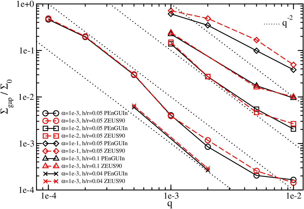
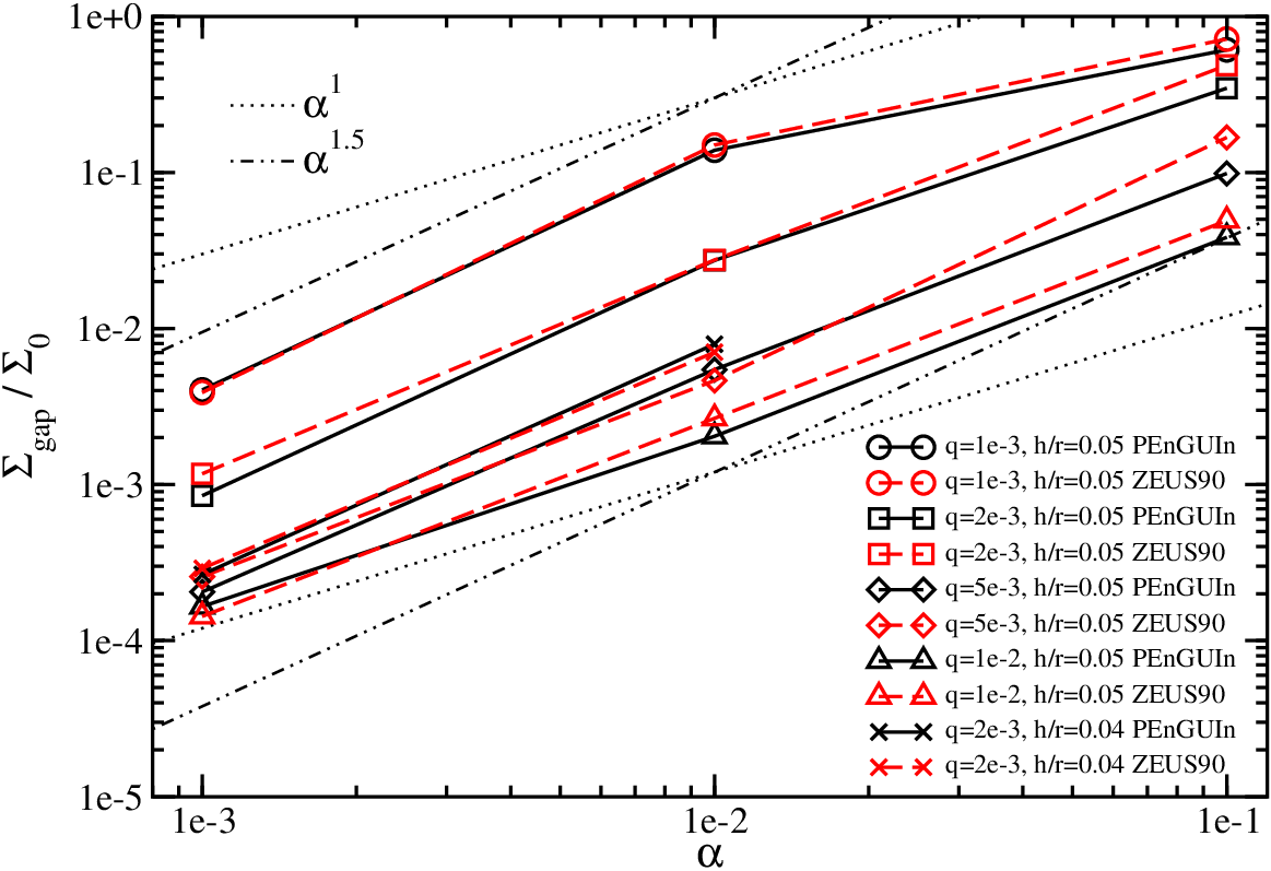
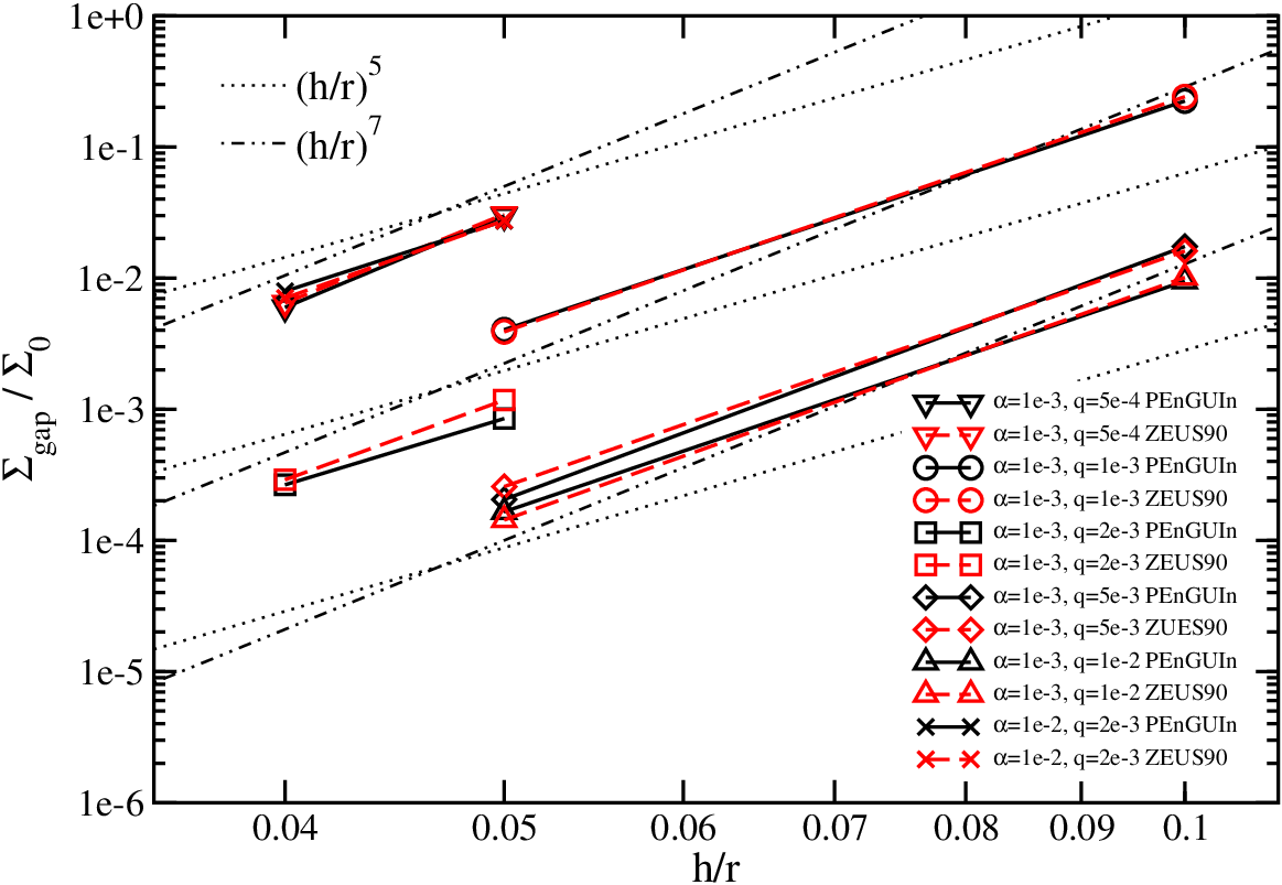
Gap depths are recorded in Table 1 and plotted against each of the parameters , , and in Figures 6, 7, and 8, respectively. Overall the agreement between the two codes, which utilize completely different algorithms, is remarkably good.
Figure 6 attests that for , gap depths scale roughly as — as our analytic scaling (3) predicts. For , the curves flatten somewhat (more on the behavior at large in §III.2). In Figure 7, appears to scale with to a power between 1 and 1.5. For comparison, our analytic scaling (3) predicts . The empirical dependence on is similarly steeper than the analytic dependence: equation (3) predicts that whereas Figure 8 shows that the power-law indices vary between 5 and 7.
We obtain a “best-fit” power-law relation by minimizing the function over the parameters . The sum is performed over data points, excluding the discrepant runs at and runs for which (i.e., runs for which gaps hardly open). With these exclusions, there are data points from PEnGUIn, best fitted by
| (12) |
The points from ZEUS90 are best described by a very similar formula:
| (13) |
Both of these relations fit their respective data to typically better than 20%; the largest deviation in the PEnGUIn fit is 40%, corresponding to , and for ZEUS90 the largest deviation is 50%, corresponding to .
Because our two codes agree so well, and because the fits are good, we are confident the deviations between our empirical scaling (say equation 12 from PEnGUIn) and our analytic scaling (3) are real and reflect physical effects not captured by our analytic scaling. And because our analytic scaling (3) matches exactly the scalings found numerically by Duffell and MacFadyen [15] at low — whereas our empirical relation (12) applies to high --- these physical effects manifest for giant (Jupiter-like) planets, not lower-mass (Neptune-like) planets.44 4 Another difference between our simulations and theirs is that we mandate a steady across our entire domain, whereas they adopt (as appears customary for work in this field) wave-killing zones that effectively result in nearly zero-inflow boundary conditions. We have verified, however, that this difference does not matter for ; we implemented zero-inflow boundaries in a few runs with PEnGUIn and found results for that matched those with our standard accreting boundaries to better than 1%. We have not elucidated what this physics is, although there might be some clues from the gap behavior at the very highest values of we tested, as discussed in §III.2.
At the same time, we emphasize that the deviations between (3) and (12), though (probably) real, are not large. If we insist on fitting the PEnGUIn data using (3) — i.e., if we fix and allow only the coefficient to float — then the data deviate from (3) by typically a factor of 2, and at most a factor of 3. Thus the physical effects not captured by our analytic scaling, whatever they are, do not lead to order-of-magnitude changes in gap depth, at least over the range of parameters tested.
III.2. Behavior of Gaps at High
The dependence of on flattens at the highest values of considered (Figure 6). Fitting the points from PEnGUIn for which and yields:
| (14) |
Similarly for the points from ZEUS90 we obtain:
| (15) |
Although at first glance one might attribute the flattening of the trend of with to the onset of strong shocks, we do not believe this is the correct interpretation. In the strong-shock regime, where disturbances excited by the planet are non-linear at launch, the torque exerted on the disk by the planet scales as (e.g., Hopkins and Quataert 28, their section 2.3).55 5 This scaling can be seen by replacing with in equation (1); the torque cut-off distance generally equals , which in the strong-shock limit equals . Then the same arguments in §I.1 yield . This analytic relation reproduces the scaling index for given by our empirical relations (14) and (15), but fails to reproduce the empirical scaling index for . Furthermore, the flattening begins at an apparently “universal” -value of that is independent of , whereas in the strong-shock interpretation, the critical -value should scale as (i.e., the expected critical is given by the so-called thermal mass).
We do not have an explanation for the flatter slope of at high . We speculate that it might be caused by the most massive companions causing material at the gap edge to “leak” into the gap. The most massive planets disturb the gap edge so strongly that local instabilities send streamers of gas into the gap. These streamers, which de Val-Borro et al. [25] called “filaments”, are prominent in the high- snapshots in Figure 9 (and can be seen even at in the PEnGUIn snapshot in Figure 3). The filaments appear to originate from unsteady structures along gap edges; similar structures were seen by, e.g., Kley & Dirksen (2006, their figures 1 and 7).

We also observe evidence for an eccentric outer disk at high ; see Figure 10 and the “Comments” column in Table 1. The outward transport of angular momentum by waves launched at the 1:3 outer eccentric Lindblad resonance pumps the eccentricity of the outer disk [30, 31]. The -value for which disks become eccentric depends on , , and disk mass [30, 31, 29, 32, 33]. For a planet held on a fixed circular orbit embedded in a non-gravitating disk for which and , [29] found that led to eccentric disks; for , the required . Their findings are in line with ours.
In two runs with PEnGUIn, an eccentricity appears in the outer disk at early times but damps away by the time converges (see Table 1). The eccentricity damping is probably an artifact of our outer circular boundary at , which according to [29] is too close to the planet to properly simulate eccentric disks. The danger posed by the outer boundary should lessen as the -viscosity increases and disturbances excited by the planet are more localized; this may be why circularization occurs only for our lowest runs at high .
We note that the fine-structure filaments threading the gaps are seen in most of our simulations, while only a few of these cases evince eccentric outer disks. Moreover, the filaments observed by [25] do not appear associated with disk eccentricity. It is unclear to us whether the filaments and disk eccentricity are directly related.


III.3. Code Comparison
Generally PEnGUIn and ZEUS90 agree very well on (e.g., Figures 6–8), typically differing by no more than a few tens of percent, and often much better. Because the codes rely on fundamentally different algorithms — one is a shock-capturing Lagrangian-remap code, while the other is an Eulerian code using the upwind method — their agreement lends confidence in the accuracy of our results. Some minor, systematic differences include: (i) for ZEUS90 is larger than for PEnGUIn; (ii) PEnGUIn usually resolves a higher density peak near the planet; (iii) PEnGUIn typically requires a longer time to converge; and (iv) near the outer boundary where the resolution is coarser, ZEUS90 has difficulty relaxing to the steadily accreting solution described by equations (9)–(11), deviating from the correct by up to 50%. All of these differences may be attributed to the fact that PEnGUIn uses PPM, which is a fourth-order method for uniform grids (third-order for non-uniform grids), whereas ZEUS90’s algorithm is only second-order in space. Thus PEnGUIn tends to be more accurate and less numerically diffusive than ZEUS90, at the cost of taking a longer time to resolve sharp features.
A key innovation of PEnGUIn is its use of GPU technology to accelerate computations. PEnGUIn’s speed on a single GTX-Titan graphics card can rival that of a traditional CPU cluster having 100 cores. For this paper we ran PEnGUIn on a desktop computer housing 3 graphics cards. With specialized hardware we can connect up to 8 GPUs to a motherboard. PEnGUIn’s scalability with the number of cards approaches linear as the resolution increases; our speed on 3 cards is 2.33 that of a single card at our standard resolution; if the resolution is doubled (quadrupled), the speed enhancement factor increases to 2.64 (2.92) as PEnGUIn takes more full advantage of GPU’s parallelism. Currently PEnGUIn can run on a single node only, and would need to be modified to run on multiple nodes. In a multi-node cluster of GPUs, the scaling of speed with the number of cards per node is unlikely to be linear because communication between nodes is significantly slower than between cards on a single node.
IV. CONCLUSIONS AND OUTLOOK
We established two empirical formulas (12 and 14) for the surface density contrast, , inside and outside the gap carved by a non-accreting giant planet. The first is valid for planet-to-star mass ratios , and the second is valid for . Our formulae are derived from our new, fast, Lagrangian shock-capturing PPM code PEnGUIn, and are confirmed by ZEUS90. Combining our results with those from the literature, we find that scales with , viscosity parameter , and disk aspect ratio in the following ways:
- •
At Neptune-like (and perhaps lower) masses, [15] found66 6 A caveat is that [15] did not explicitly test the dependence on that they proposed. We used PEnGUIn to try to reproduce their low-mass results (data not shown), but encountered the problem that took too long to converge. What low-mass data we did collect at the end of orbital periods were consistent with the power-law indices proposed by [15]. that ;
- •
At Jupiter-like masses, we find that (our equation 12);
- •
At masses near the brown dwarf threshold, we find that (our equation 14).
Our scaling indices for giant planets and quasi-brown dwarfs are supported by two independent codes using different algorithms, and so we are confident in their accuracy. Note that our simulations and those of Duffell and MacFadyen [15] do share one common set of parameters: , for which we find and they find (their Figure 2).77 7 Technically, our simulations have spatially constant and , whereas theirs has spatially constant and . Also, we compute as an area average, whereas they report the minimum surface density. These differences are probably immaterial. We consider this good agreement.
The scaling differences between low mass and high mass, although pointing to real physical effects, do not lead to order-of-magnitude changes in gap depth, at least over the range of parameters surveyed. That is, using the Neptune-like scaling for Jupiter-like planets leads to gap depths that differ (systematically) from those observed in our simulations by factors of only 2–3.
IV.1. Connecting to Observations of Transition Disks
Are the gaps empty enough to reproduce the low optical depths characterizing the cavities of transitional and pre-transitional disks? Surface density contrasts from models of disks like PDS 70 [8] and GM Aur [34] are or more. We have found that certain sets of planet-disk parameters can achieve such contrasts. For example, produces contrasts of 5000 (Table 1). Lower mass planets could also be made to work with lower -viscosities and/or cooler disks with lower ; as a further example, generates a contrast of 3000. The dependence on disk temperature is especially sensitive: .
The surface density contrasts reported in this paper are all underestimates insofar as we have neglected accretion onto the planet; but arguably the disk accretion rate cannot be reduced by more than a factor of order unity, lest the planet starve the host star and violate observed stellar accretion rates (Zhu et al. 5; see also Lubow and D’Angelo 12). We would argue further that our gas surface density contrasts are also underestimates of dust surface density (i.e., optical depth) contrasts, to the extent that mechanisms like dust filtration at outer gap edges (e.g., Zhu et al. 7) deplete dust relative to gas in gaps.
Given these findings, we feel that when it comes to transition disks, the problem is not so much gap depth, but gap width. A single planet embedded in an accreting disk generates a gap too narrow in radial width to explain the expansive cavities observed in transition disks. To connect to observations would seem to require that we expand our study to include multiple planets or brown dwarfs within a viscous, gravitating disk, as has been done by Zhu et al. [5]. These authors discounted — and were therefore compelled to invoke additional channels of opacity reduction (e.g., grain growth) to explain transition disks — because multiple planets were found to be dynamically unstable at low / high (see their page 8). The incompatibility of multiple giant planets with low is a result that we would like to see confirmed independently and further explored.
IV.2. A Floor on
All our empirical scalings for suggest that arbitrarily low values of generate arbitrarily clean gaps. We expect, however, the scalings to break down for small enough . Without an intrinsic disk viscosity, a planet may stir the gap edge in such a way as to trigger local instabilities and turbulent diffusion. For example, with , the outer gap edge might be so sharp as to be Rayleigh unstable. There should therefore be a minimum value or “floor” on caused by a minimum planet-driven viscosity. Just such a floor has been reported by [15]; see their Figure 7. Other simulations of planets in inviscid disks, concentrating on orbital migration and not gap depth, have been carried out by [35] and [36].
Similar arguments suggest that there might also be a floor on at high . The streamers/filaments that invade the gap are densest for the highest -values we tested.
IV.3. Analytic Derivation
In §I.1, we presented an analytic derivation of gap depth . We discovered that the power-law scalings in our analytic relation (3) match precisely those reported from numerical experiments for low-mass planets by Duffell and MacFadyen [15]. Our analytic relation can even reproduce approximately (deviating systematically by factors of a few) the empirical results we found for gaps carved by Jupiter-like planets.
The success of our breezy analytic derivation for is surprising. Our derivation is “zero-dimensional” (“0D”) because it considers only the total rates of angular momentum transport – a.k.a. the total “angular momentum luminosity” or “angular momentum current” — integrated over all azimuth and radius; it ignores the complicated details of how the torques are actually applied differentially in space. We have already noted in §I.1 how it is not completely obvious that characterizes the viscous torques in gap edges. Furthermore, our 0D treatment considers only the wave and viscous contributions to the total angular momentum current, and neglects the contribution from advection (i.e., the transport of angular momentum associated with a non-zero radial velocity ) and the contribution from azimuthal pressure variations [11].
We can address some of these problems and make the leap from 0D to 1D by considering the azimuthally averaged, radially dependent torque balance equation for a steady-state accretion disk perturbed by a planet (see, e.g., equation 3 of Lubow and D’Angelo 12):
| (16) |
where the Lindblad torque per unit mass is
| (17) |
and is an order-unity constant. The left-hand side of (16) accounts for the viscous torque, while the first term on the right-hand side accounts for angular momentum transport by advection. We define and constant , and approximate so that = constant (variables subscripted by take their values at the planet’s orbital radius). For the outer disk, equation (16) simplifies to
| (18) |
From this equation it becomes apparent how the outer accretion disk responds when repelled outward by a planet: for , the surface density gradient steepens, just enough that the viscous torque can exceed the Lindblad torque and maintain a steady flow of mass inward (i.e., carry the imposed at infinity across the planet’s orbit).
Setting , and working in the WKB limit where , gives the standard zero-inflow solution: an exponential profile for , commonly used in the literature (e.g., Lubow et al. 24; de Val-Borro et al. 37; Mulders et al. 38). Keeping alters : it still resembles an exponential but is shifted outward (for fixed ), as Figure 12 demonstrates. We find for the parameters chosen that equation (18) describes well the gap profile from our 2D simulations, down to a distance of 3–4 Hill radii away from the planet. But inside this cut-off distance, the 1D solution fails critically — it falls much too steeply to recover the actual flat-bottomed gap.
The problem of determining the gap depth analytically in 1D appears tantamount to the problem of understanding what happens inside this cut-off distance. Lindblad torques shut off here; the tidal gravitational field of the planet is especially strong; and circulating streamlines give way to horseshoe orbits. One-dimensional analytic treatments may be inadequate to the task of modeling how gas navigates from the outer disk to the inner disk through a series of “horseshoe turns” [24, 9]. As far as analytic treatments go, it may be that to do better than 0D requires at least 2D.

References
- [1] P. Goldreich and S. Tremaine, ApJ 241, 425 (1980).
- [2] A. L. Kraus and M. J. Ireland, ApJ 745, 5 (2012).
- [3] J. H. Debes, H. Jang-Condell, A. J. Weinberger, A. Roberge, and G. Schneider, ApJ 771, 45 (2013).
- [4] S. P. Quanz, H. Avenhaus, E. Buenzli, A. Garufi, H. M. Schmid, and S. Wolf, ApJ 766, L2 (2013).
- [5] Z. Zhu, R. P. Nelson, L. Hartmann, C. Espaillat, and N. Calvet, ApJ 729, 47 (2011).
- [6] S. E. Dodson-Robinson and C. Salyk, ApJ 738, 131 (2011).
- [7] Z. Zhu, R. P. Nelson, R. Dong, C. Espaillat, and L. Hartmann, ApJ 755, 6 (2012).
- [8] R. Dong, J. Hashimoto, R. Rafikov, Z. Zhu, B. Whitney, T. Kudo, T. Muto, T. Brandt, M. K. McClure, J. Wisniewski, et al., ApJ 760, 111 (2012).
- [9] W. Kley and R. P. Nelson, ARA&A 50, 211 (2012).
- [10] W. R. Ward, ApJ 482, L211 (1997).
- [11] A. Crida, A. Morbidelli, and F. Masset, Icarus 181, 587 (2006).
- [12] S. H. Lubow and G. D’Angelo, ApJ 641, 526 (2006).
- [13] J. M. Stone and M. L. Norman, ApJS 80, 753 (1992).
- [14] J. Frank, A. King, and D. Raine, Accretion Power in Astrophysics (Cambridge Astrophysics) (Cambridge University Press, 2002), ISBN 0521620538.
- [15] P. C. Duffell and A. I. MacFadyen, ApJ 769, 41 (2013).
- [16] N. I. Shakura and R. A. Sunyaev, A&A 24, 337 (1973).
- [17] P. Colella and P. R. Woodward, Journal of Computational Physics 54, 174 (1984).
- [18] J. M. Blondin and E. A. Lufkin, ApJS 88, 589 (1993).
- [19] D. S. Balsara, ApJ 420, 197 (1994).
- [20] W. Kley, A&A 338, L37 (1998).
- [21] J. F. Hawley and J. M. Stone, Computer Physics Communications 89, 127 (1995).
- [22] J.-M. Shi, J. H. Krolik, S. H. Lubow, and J. F. Hawley, The Astrophysical Journal 749, 118 (2012).
- [23] K. A. Sorathia, J. H. Krolik, and J. F. Hawley, The Astrophysical Journal 768, 133 (2013).
- [24] S. H. Lubow, M. Seibert, and P. Artymowicz, ApJ 526, 1001 (1999).
- [25] M. de Val-Borro, R. G. Edgar, P. Artymowicz, P. Ciecielag, P. Cresswell, G. D’Angelo, E. J. Delgado-Donate, G. Dirksen, S. Fromang, A. Gawryszczak, et al., MNRAS 370, 529 (2006).
- [26] J. Goodman and R. R. Rafikov, ApJ 552, 793 (2001).
- [27] T. W. A. Müller, W. Kley, and F. Meru, A&A 541, A123 (2012).
- [28] P. F. Hopkins and E. Quataert, MNRAS 415, 1027 (2011).
- [29] W. Kley and G. Dirksen, A&A 447, 369 (2006).
- [30] S. H. Lubow, ApJ 381, 259 (1991).
- [31] J. C. B. Papaloizou, R. P. Nelson, and F. Masset, A&A 366, 263 (2001).
- [32] G. D’Angelo, S. H. Lubow, and M. R. Bate, ApJ 652, 1698 (2006).
- [33] A. C. Dunhill, R. D. Alexander, and P. J. Armitage, MNRAS 428, 3072 (2013).
- [34] N. Calvet, P. D’Alessio, D. M. Watson, R. Franco-Hernández, E. Furlan, J. Green, P. M. Sutter, W. J. Forrest, L. Hartmann, K. I. Uchida, et al., ApJ 630, L185 (2005).
- [35] H. Li, S. H. Lubow, S. Li, and D. N. C. Lin, ApJ 690, L52 (2009).
- [36] C. Yu, H. Li, S. Li, S. H. Lubow, and D. N. C. Lin, ApJ 712, 198 (2010).
- [37] M. de Val-Borro, P. Artymowicz, G. D’Angelo, and A. Peplinski, A&A 471, 1043 (2007).
- [38] G. D. Mulders, S.-J. Paardekooper, O. Panić, C. Dominik, R. van Boekel, and T. Ratzka, A&A 557, A68 (2013).