跳到论文正文
W Papers独立论文阅读器 arXiv:1309.7960 论文正文 计算阅读时间 · 0%
引用这篇论文根据当前论文元数据生成,正式投稿前建议核对。


License: arXiv.org perpetual non-exclusive license
arXiv:1309.7960v2 [math.DG] 29 Aug 2014

A Classification of Configuration Spaces of Planar Robot Arms
with Application to a Continuous Inverse Kinematics Problem

Subhrajit Bhattacharya ††thanks: Department of Mathematics, University of Pennsylvania, Philadelphia PA 19104. e-mail: subhrabh@math.upenn.edu. Phone: (001) 267-252-6638. (Corresponding aothor).    Mihail Pivtoraiko ††thanks: Department of Mechanical Engineering and Applied Mechanics, University of Pennsylvania, Philadelphia PA 19104. e-mail: mihailp@seas.upenn.edu
Abstract

Using results on the topology of moduli space of polygons [10, 12], it can be shown that for a planar robot arm with nn segments there are some values of the base-length, zz (i.e., length of line joining the base of the arm with its end-effector), at which the configuration space of the constrained arm (arm with its end effector fixed) has two disconnected components, while there are other values at which the constrained configuration space has one connected component. We first review some of these known results relating the value of zz with the connectivity of the constrained configuration space with end-effector fixed.

Then the main design problem addressed in this paper is the construction of pairs of continuous inverse kinematics for arbitrary robot arms, with the property that the two inverse kinematics agree (i.e. return the same configuration) when the constrained configuration space has a single connected component, but they give distinct configurations (one in each connected component) when the configuration space of the constrained arm has two components. This design is made possible by a fundamental theoretical contribution in this paper – a classification of configuration spaces of robot arms such that the type of path that the system (robot arm) takes through certain critical values of the forward kinematics function is completely determined by the class to which the configuration space of the arm belongs. This classification result makes the aforesaid design problem tractable, making it sufficient to design a pair of inverse kinematics for each class of configuration spaces (three of them in total).

The motivation for this work comes from a more extensive problem of motion planning for the end effector of a robot arm, in which the ability to continuously sample one configuration from each connected component of the constrained configuration spaces of the arm enables us to dramatically reduce the dimensionality of the space in which the planning has to be performed, without sacrificing completeness guarantees. We start the paper with the general motivation, but address only the problem of sampling such configurations when there is no obstacle in the environment – a problem that in itself is non-trivial. Incorporating obstacles and a complete graph search-based planning for the end effector using this technique will be presented in a future papers.

We demonstrate the simplicity and the low complexity of the presented algorithm through a Javascript + HTML5 based implementation available at http://hans.math.upenn.edu/~subhrabh/nowiki/robot_arm_JS-HTML5/arm.html.

Acknowledgements: We would like to thank Prof. Vijay Kumar, Department of Mechanical Engineering and Applied Mechanics, University of Pennsylvania, and Prof. Robert Ghrist, Department of Mathematics, University of Pennsylvania, for their valuable suggestions and insightful discussions during the course of writing this paper.

1 Introduction and Related Work

In context of studying the topology of the configuration space of polygons (i.e., a robot arm with a fixed end-effector position) some remarkable results were proposed in the PhD thesis of B. Jaggi [10]. Later on, some of those results were rediscovered and enhanced in [12] and also reported in [20]. While these beautiful mathematical results are worth exploring in their own rights, in this paper we use them as a first step towards solving a very practical path planning problem for the end effector of a planar robot arm. To that end we discover a classification of configuration spaces of planar robot arms (Proposition 4 in this paper) based on how the forward kinematics function for the arm passes through certain critical values. This insight then serves as a key to solving the design problem proposed in this paper – construction of pairs of continuous inverse kinematics that give one unique configuration in each connected component of the constrained configuration spaces.

1.1 Motivation

1.1.1 General Motivation

This paper is motivated by two key needs:

  • 1.

    The need for an inverse kinematics to be continuous – That is, as we change the end effector position continuously, the joint angles computed using the IK algorithm should also change continuously and should not have abrupt jumps: In literature, for planar and spatial arms with a few segments, this has often been achieved by explicit trigonometric formulae developed from the geometry of the specific arm [22, 19]. However, very often such formulations are limited to the specific arm that the IK is designed for, becomes increasingly complex with the increase in the number of segments, and does suffer from isolated singularities and/or discontinuities. For more complex arms, traditionally numerical gradient-decent type algorithms have been used [6, 16, 5, 26]. However, the problem very often being nonlinear and non-convex, guarantees of completeness or even continuity are difficult to achieve. Furthermore, numerical techniques are often computationally expensive. A mixed numerical and analytic technique has been used in [15] for computing inverse kinematics in context of path planning for the end effector of an arm with 22 segments and point obstacles in the environment. A closed form solutions to the inverse kinematics problem has recently been hinted in [17] using a triangulation approach. But the problem being addressed for a spatial arm, some numerical techniques were also adopted.

    The IK algorithm that we propose and use in this paper is an analytically computable one of O⁡(n2)O(n^{2}) complexity (nn being the number of segments of the arm), akin to the triangulation approach of [17]. However our additional requirement of identifying and passing through certain critical points in the configuration space, as will be described in the next point, has necessitated a more careful and formal construction of the IK algorithm. In particular, our algorithm has a recursive or incremental flavor to it, wherein we construct the inverse kinematics by breaking up the arm into smaller components.

  • 2.

    Design of tuples of continuous inverse kinematics which, for a given end effector position, return only one unique configuration in every connected component of the constrained configuration space: The motivation for wanting to achieve this will be clear in the next subsection. This problem is challenging because of the plethora of geometric properties of the configuration space of a robot arm that one is faced with as the number of segments as well as the lengths of the segments are changed. In [10, 12, 20] it was proved that there are only two possible types as far as the connectivity of the constrained configuration space (i.e., the configuration space with end effector position fixed; equivalently the moduli configuration space of a polygon with (n+1)(n+1) sides) is concerned: Either it has a single connected component, or it a disjoint union of two (n−2)(n-2)-dimensional tori. Due to a fundamental theorem from Morse theory [21, 18], a continuous transition from a state in one of these types to one in the other type, that results in the change in the topology (connectivity) of the constrained configuration space, will mean that the system will pass through a critical value of the Morse function which maps configurations to the base length. We call the corresponding critical points vital critical points. In order to design the pairs of IK with the desired properties, we need to ensure that the system passes through the vital critical points at the vital critical values of the base length.

    The way we handle this design problem is to first identify the possible vital critical points for a given system, and how the system passes through the vital critical points as the base length is changed continuously. One surprising result that we derive (Proposition 4) is that there are only three such possible types of paths passing through the different vital critical points despite the large variety of robot arms that one can come up with. This essentially gives us a classification of configuration spaces of planar robot arms, and thus simplifies our problem of design of the IK pairs significantly — we only need to consider the three possible classes, and design three corresponding pairs of IKs.

1.1.2 Motivation from a Path Planning Problem

Although the aforesaid problem objectives are interesting in their own rights, in this section we elaborate on a more practical motivation for the problem that initiated this line of research in the first place. While this motivation relies largely on the presence of obstacles in the environment, we will also illustrate the non-triviality of the proposed solution even in environments without obstacle. This paper is solely dedicated to the later, while the more general case with obstacles will be considered in a forthcoming paper as discussed in Section 6.

Figure 1: The end effector of the robot arm may not follow the trajectories marked in magenta starting from the initial configuration as shown. In the left figure a trajectory in a different homotopy class (shown in green) solves the problem since it can be followed by the end effector. But not so in the case of the right one (the trajectory in red is in a different homotopy class, but still cannot be followed). In this case, a different trajectory (shown in green, which is in the same homotopy class as the magenta one), but passing through a critical configuration, can be followed. This issue is arguably endemic to environments with obstacles. However the proper solution to this problem involves sampling one configuration in each connected component of the constrained configuration spaces for different end-effector positions. And achieving that solution, even in complete absence of obstacles, involves non-trivial techniques. This paper, the first in a series, deals with solving the problem of continuously sampling one configuration from the constrained configuration spaces for each end-effector position, assuming that there is no obstacle in the environment.

The practical motivation behind this line of research comes from the recent advances in robotics, computer graphics as well as health sciences relating to kinematics of human motion and tools consting of linkages [3, 13]. The problem of inverse kinematics has been actively studied for several decades due to the many promising benefits of these applications. Often the subject of interest that leads to the inverse kinematics problem is the end-effector of the robot arm, rather than the arm itself. There may be applications in which one may need to plan shortest feasible paths for the end effector from an initial position to a final position (for example, in minimally invasive assisted laparoscopic surgery using a robotic manipulator [25], where the objective is to reach a tissue of interest inside the body). Being reduced to a typical path planning problem, a roboticist will be inclined to discretize the configuration space, place a vertex on every feasible cell in the discretization, and establish edges between neighboring vertices, thus creating a graph in which a search-based algorithm such as A* [8] or D* [24] may be employed. Such an approach has guarantees on completeness and optimality as opposed to continuous gradient-decent like approaches which suffer from issues of local minima and suboptimality [14, 11, 4]. However it is to be remembered that the configuration space of the arm is the entire space of the joint angles, which, for an arm with nn segments, is a nn-dimensional space (a nn-torus, 𝕋n\mathbb{T}^{n}, with punctures caused by presence of obstacles or infeasible arm configurations). Discretization and graph construction in such a high dimensional configuration space creates an extremely large graph with high degree (number of emanating edges) per vertex. While such graphs have indeed been used in solving the path planning problem for planar robotic arms [9], typically a full-blown search being highly expensive, a compromise has to be made in the optimality of the search result or the completeness of the algorithm using randomized techniques like the ARA* algorithm.

One may attempt to simplify the problem by instead trying to plan a trajectory in the 22-dimensional space of the end-effector, (ℝ2−𝒪)(\mathbb{R}^{2}-\mathcal{O}) (where 𝒪\mathcal{O} is the set of obstacles), and hence try to make the arm move (using, for example, a feedback controller) such that the end effector follows the planned trajectory. However very often the arm will fail to follow such a planned trajectory, even though every point on the trajectory is reachable (see Figure 1 and Section 3.6.1 of [1]).

One may try to resolve this issue by planning multiple trajectories in the different homotopy classes in (ℝ2−𝒪)(\mathbb{R}^{2}-\mathcal{O}) (the multiple homotopy classes being created due to the presence of obstacle) as was discussed in [1, 2]. However a close investigation reveals that this approach is not enough (for example the case on the right in Figure 1).

We proposed the correct solution approach to be the following:

Given an end-effector position, we sample exactly one configuration from every connected component of the constrained configuration space (recall that the constrained configuration space is the configuration space of the arm with the end effector fixed, which, in presence of obstacles, will exclude configurations in which a segment of the arm intersects an obstacle). As the end effector is moved in a continuous fashion, the sampled points from the configuration space will obviously change, but it should change continuously as well. This leads to the notion of a ‘proximity’ among the different sampled configurations as the end effector position is changed. A graph can hence be created — vertices correspond to sampled configurations from constrained configuration spaces for every discrete end-effector positions, and edges are established between adjacent configurations (that is, the corresponding sampled configurations for the adjacent end-effector positions).

Since for every end effector position we sample a finite number of distinct configurations (one for each connected component of the constrained configuration space), the set of all the sampled configuration is a space with the same dimensionality as the end effector space (but with a different topology, akin to the topology of a covering space [7]). Thus we have reduced the dimensionality of the problem significantly from the one encountered when planning in the entrire nn-dimensional configuration space of the arm. It is however worth noting that within a connected component of a constrained configuration space every configuration can be reached from the other keeping the end effector fixed. Thus sampling one configuration from each connected component gives us a faithful low-dimensional representation of the nn-dimensional joint space. This is illustrated in Figure 2.

Figure 2: (Informal/schematic diagram for illustration) The idea behind creating a faithful low-dimensional representation of the configuration space by sampling one point from each connected component of every constrained configuration space. The sampled subspace can be constructed as union of the image of multiple inverses kinematics (maps from end-effector space to configuration space) passing through certain critical points in the configuration space.

Due to the above, it is in fact easy to observe that there exists a path in the full configuration space of the arm, whose image under the end-effector map (i.e., the map that takes in a configuration and returns the corresponding end-effector position) is a given trajectory, if and only if there also exists a path in the subspace consisting of the sampled points whose image under the end-effector map is the same trajectory. Thus we end up reducing the dimensionality of the problem without compromising the completeness guarantees.

The non-triviality even in absence of obstacles in the environment: Although the illustrations and the rationales described above may indicate that obstacles are the only culprits in making a constrained configuration space have disconnected components and hence the need for the continuous sampling as described, that in fact is not true. Due to the results of [10, 12], even when there is no obstacle in the environment, a constrained configuration space may have one or two connected components. In this paper we design a way of continuously sampling one configuration from each connected component of the constrained configuration spaces as described, and as the first step, we assume that there is no obstacle in the workspace. We moreover assume that there is no joint limit and the the segments of the arm lie in different planes so that there is no self-collision of the arm. As we will see, this problem in itself is highly non-trivial. This is the first paper in a planned series, where the eventual objective will be to extend the techniques developed in this paper to environments with obstacles and arms with joint limits, and hence be able to execute graph search algorithms to do quick and efficient planning for robot arms with completeness guarantees.

1.2 Organization of the Paper

We start with some well-known results and simple observations in Section 2. Following this, the main content of the paper is organized into two sections: i. Section 3 describes a general continuous inverse kinematics map that involves choice of certain parameters, and, ii. the main contributions of the paper appear in Section 4, where we describe how to choose the said parameters for designing the IK pairs with the desired property (one unique configuration per connected component of the constrained configuration space). The later is made possible by the main theoretical contribution of the paper – the classification result of Proposition 4 – where we identify the possible types of paths that a system can take through the vital critical values of the base-length function. The main technical contribution of the paper is summarized in Proposition 5.

2 Preliminaries

Figure 3: A general planar arm at a configuration that is in its restricted configuration space, ℜ⊂𝕋m\mathfrak{R}\subset\mathbb{T}^{m}.

The configuration space of a nn-segmented planar robot arm is the nn-torus, 𝕋n\mathbb{T}^{n}, which we coordinatize using the angles that the segments of the arm make with the positive XX axis (see Figure 3). Thus, [θn−1,θn−2,⋯,θ0][\theta_{n-1},\theta_{n-2},\cdots,\theta_{0}], with θi∈𝕊1\theta_{i}\in\mathbb{S}^{1}, gives an unique configuration of the arm.

Throughout the paper we will assume that the end effector of the arm can be at points q∈(ℝ2−{0})q\in(\mathbb{R}^{2}-\{0\}), where {0}\{0\} is the location of the fixed base of the arm. That is, we eliminate the cases when the end effector of the robot arm coincides with the base (equivalently, the base-length, zz, vanishes). Thus the configuration space that is of interest to us is (𝕋n−O~)(\mathbb{T}^{n}-\tilde{O}), where 𝕋n⊃O~={[θn−1,θn−2,⋯,θ0]∈𝕋n|∑i=0n−1li​sin⁡(θi)=∑i=0n−1li​cos⁡(θi)=0}\mathbb{T}^{n}\supset\tilde{O}=\{[\theta_{n-1},\theta_{n-2},\cdots,\theta_{0}]\in\mathbb{T}^{n}~\big|~\sum_{i=0}^{n-1}l_{i}\sin(\theta_{i})=\sum_{i=0}^{n-1}l_{i}\cos(\theta_{i})=0\}.

2.1 The Restricted Configuration Space of a Planar Robot Arm

The first observation that one can make is that it is sufficient to study the configuration space of the arm up to an equivalence, ‘∼\sim’, of rotations of the entire arm about the base (see [10] – in fact the equivalence can be extended to translations and scalings of the arm as discussed in [12] – transformations that are however not relevant to a robot arm). In particular, this lets us design inverse kinematics assuming that the end effector will always lie on the positive XX axis. The corresponding set of configurations (a subspace of the complete configuration space of interest, (𝕋n−O~)(\mathbb{T}^{n}-\tilde{O})) will constitute the restricted configuration space, ℜ\mathfrak{R}.

The sufficiency in focusing on ℜ\mathfrak{R} follows from the simple observation that given any arbitrary configuration of the arm, C∈(𝕋n−O~)C\in(\mathbb{T}^{n}-\tilde{O}), we can rotate the entire arm about the base by an angle, −ρ-\rho, (ρ=atan2​(qy,qx)∈𝕊1\rho=\text{atan2}(q_{y},q_{x})\in\mathbb{S}^{1} being the angle that the base segment makes with the positive XX axis) and the resulting configuration will have the end effector on the positive XX axis. Furthermore, this rotation, −ρ-\rho, depends only on the end effector position and not on the entire configuration, CC. Thus, given only an end effector position, q=[qx,qy]T∈ℝ2−{0}q=[q_{x},q_{y}]^{T}\in\mathbb{R}^{2}-\{0\}, we can compute the required rotation, following which we compute a configuration K∈ℜK\in\mathfrak{R} (using an inverse kinematics, IK:ℝ+→ℜ\mathrm{IK}:\mathbb{R}_{+}\rightarrow\mathfrak{R}) such that the end effector is on the positive XX axis at a distance of z=‖q‖=qx2+qy2z=\|q\|=\sqrt{q_{x}^{2}+q_{y}^{2}} from the base, and thus rotate KK by an angle of ρ\rho to get a configuration, C∈(𝕋n−O~)C\in(\mathbb{T}^{n}-\tilde{O}), with end effector at qq (see Figure 4). Furthermore, if IK:ℝ+→ℜ\mathrm{IK}:\mathbb{R}_{+}\rightarrow\mathfrak{R} is continuous/differentiable, so will be this sequence of maps involving the rotations.

Refer to caption
Figure 4: A continuous inverse kinematics for the entire configuration space of the arm, (𝕋n−O~)→(ℝ2−{0})(\mathbb{T}^{n}-\tilde{O})\rightarrow(\mathbb{R}^{2}-\{0\}), can always be constructed from a continuous inverse kinematics on the restricted configuration space, ℜ→ℝ+\mathfrak{R}\rightarrow\mathbb{R}_{+}. This gives the rationale behind why it is sufficient to consider the restricted configuration space instead of the entire configuration space of the arm.

Thus, in all the following discussions we will only consider configurations such that the end effector lies on a reference ray (positive XX axis is chosen for convenience). We write ℜ⊂(𝕋n−O~)\mathfrak{R}\subset(\mathbb{T}^{n}-\tilde{O}) to denote this configuration space, and call it the restricted configuration space. In terms of coordinates, if we coordinatize the 𝕋n\mathbb{T}^{n} by the angles that the segments (say of lengths ln−1,ln−2,⋯,l0l_{n-1},l_{n-2},\cdots,l_{0}) make with the positive XX axis, [θn−1,θn−2,⋯,θ0][\theta_{n-1},\theta_{n-2},\cdots,\theta_{0}], then ℜ\mathfrak{R} denotes the subspace satisfying the condition qy=∑j=0n−1lj​sin⁡(θj)=0,qx=∑j=0n−1lj​cos⁡(θj)>0q_{y}=\sum_{j=0}^{n-1}l_{j}\sin(\theta_{j})=0,~q_{x}=\sum_{j=0}^{n-1}l_{j}\cos(\theta_{j})>0. We will use the induced coordinatization for ℜ\mathfrak{R} — the standard coordinates on its embedding space 𝕋n\mathbb{T}^{n}, defined by the orientations of segments.

Note 1.

More formally, there exists a trivial fibration [23] of the configuration space, (𝕋n−O~)=𝕊1×ℜ(\mathbb{T}^{n}-\tilde{O})=\mathbb{S}^{1}\times\mathfrak{R} (with projection map 𝗉:(𝕋n−O~)→ℜ\mathsf{p}:(\mathbb{T}^{n}-\tilde{O})\rightarrow\mathfrak{R}, considered as a principal 𝕊1\mathbb{S}^{1} bundle), and a trivial fibration of the end-effector space, (ℝ2−{0})=𝕊1×ℝ+(\mathbb{R}^{2}-\{0\})=\mathbb{S}^{1}\times\mathbb{R}_{+} (with projection map 𝗉′:(ℝ2−{0})→ℝ+\mathsf{p}^{\prime}:(\mathbb{R}^{2}-\{0\})\rightarrow\mathbb{R}_{+}, considered as a principal 𝕊1\mathbb{S}^{1} bundle).

The end-effector map D:ℜ→ℝ+D:\mathfrak{R}\rightarrow\mathbb{R}_{+} is a map between the bases spaces, and a pullback of the later bundle under this map gives the former one. Define the resulting bundle map D^:(𝕋n−O~)→(ℝ2−{0})\widehat{D}:(\mathbb{T}^{n}-\tilde{O})\rightarrow(\mathbb{R}^{2}-\{0\}). Thus the following relation holds (by definition of pullback bundle): 𝗉′∘D^=D∘𝗉\mathsf{p}^{\prime}\circ\widehat{D}=D\circ\mathsf{p}.

The bundles being trivial, D^\widehat{D} and DD also relates as D^=Id𝕊1×D\widehat{D}=\mathrm{Id}_{\mathbb{S}^{1}}\times D. Thus, if there is a map I​K:ℝ+→ℜIK:\mathbb{R}_{+}\rightarrow\mathfrak{R} such that D∘I​K=Idℝ+D\circ IK=\mathrm{Id}_{\mathbb{R}_{+}}, then defining I​K^=Id𝕊1×I​K:(ℝ2−{0})→(𝕋n−O~)\widehat{IK}=\mathrm{Id}_{\mathbb{S}^{1}}\times IK:~(\mathbb{R}^{2}-\{0\})\rightarrow(\mathbb{T}^{n}-\tilde{O}), we can observe D^∘I​K^=(Id𝕊1×D)∘(Id𝕊1×I​K)=Id𝕊1×Idℝ+=Id(ℝ2−{0})\widehat{D}\circ\widehat{IK}=(\mathrm{Id}_{\mathbb{S}^{1}}\times D)\circ(\mathrm{Id}_{\mathbb{S}^{1}}\times IK)=\mathrm{Id}_{\mathbb{S}^{1}}\times\mathrm{Id}_{\mathbb{R}_{+}}=\mathrm{Id}_{(\mathbb{R}^{2}-\{0\})}. There are couple of immediate consequences of the above observations:

  • i.

    If I​KIK is of differentiability class CαC^{\alpha}, so is I​K^\widehat{IK}.

  • ii.

    If z∈ℝ+z\in\mathbb{R}_{+} and q∈(ℝ2−{0})q\in(\mathbb{R}^{2}-\{0\}) relate as 𝗉′​(q)=z\mathsf{p}^{\prime}(q)=z, then there is a homeomorphism between D−1​(z)⊂ℜD^{-1}(z)\subset\mathfrak{R} and D^−1​(q)⊂(𝕋n−O~)\widehat{D}^{-1}(q)\subset(\mathbb{T}^{n}-\tilde{O}) given by 𝗉|D^−1​(q):D^−1​(q)→D−1​(z)\mathsf{p}\big|_{\widehat{D}^{-1}(q)}:\widehat{D}^{-1}(q)\rightarrow D^{-1}(z). Thus the topology of D−1​(z)D^{-1}(z) is same as the topology of D^−1​(q)\widehat{D}^{-1}(q) whenever 𝗉′​(q)=z\mathsf{p}^{\prime}(q)=z.

Thus it will be sufficient to study the map DD and construct a map as I​KIK instead of studying the ‘hatted’ versions of the same. We will refrain from more detailed discussion or formal proofs of the above statements in order to remain focused on the main topic of the paper.

2.2 Number of Connected Components of Configuration Space for Fixed Base-Length

We are given a robot arm, RR, with mm segments and segment lengths lm−1,lm−2,⋯,l0l_{m-1},l_{m-2},\cdots,l_{0} (respectively starting from the base – Figure 3). Suppose the length of the base segment (i.e., the line joining the origin and the end-effector) is zz. We denote the map from the space of restricted configurations to the distance between the origin and the end effector as DR:ℜ→ℝ+,[θm−1,θm−2,⋯,θ0]↦zD_{R}:\mathfrak{R}\rightarrow\mathbb{R}_{+},~[\theta_{m-1},\theta_{m-2},\cdots,\theta_{0}]\mapsto z. Due to Lemma 2 of [10], this is a Morse function.

Now, consider the set of lengths of the sides of the closed polygon formed by the the segments of the arm and the base segment: {z,lm−1,lm−2,⋯,l0}\{z,~l_{m-1},l_{m-2},\cdots,l_{0}\} (thus, it is a polygon with m+1m+1 sides). The elements of this set, when ordered according to their value, are written as l⟨m⟩≥l⟨m−1⟩≥l⟨m−2⟩≥⋯≥l⟨1⟩≥l⟨0⟩l_{\langle{m}\rangle}\geq l_{\langle{m-1}\rangle}\geq l_{\langle{m-2}\rangle}\geq\cdots\geq l_{\langle{1}\rangle}\geq l_{\langle{0}\rangle}. Thus, l⟨m⟩=max⁡{z,lm−1,lm−2,⋯,l0}l_{\langle{m}\rangle}=\max\{z,~l_{m-1},l_{m-2},\cdots,l_{0}\}, and so on. The following result follows from Theorem 6 of [10] and Theorem 1 of [12]:

Theorem 1 ([10, 12]).

Keeping the end-effector of the arm fixed at a distance zz from the origin, and defining l⟨i⟩l_{\langle{i}\rangle} as above,

  • i

    The constrained configuration space, DR−1​(z)D_{R}^{-1}(z), is connected iff

    l⟨m⟩+∑j=0m−3l⟨j⟩≥l⟨m−1⟩+l⟨m−2⟩l_{\langle{m}\rangle}~+~\sum_{j=0}^{m-3}l_{\langle{j}\rangle}~~\geq~~l_{\langle{m-1}\rangle}~+~l_{\langle{m-2}\rangle}
  • ii

    The constrained configuration space, DR−1​(z)D_{R}^{-1}(z), is not connected (and is a disjoint union of two (m−2)(m-2)-dimensional tori) iff

    l⟨m⟩+∑j=0m−3l⟨j⟩<l⟨m−1⟩+l⟨m−2⟩l_{\langle{m}\rangle}~+~\sum_{j=0}^{m-3}l_{\langle{j}\rangle}~~<~~l_{\langle{m-1}\rangle}~+~l_{\langle{m-2}\rangle}

We will use a simple analogy for interpreting the above result, and hence motivate our forthcoming problem objectives. For simplicity (and for the sake of visualization), we consider the 22-torus, 𝕋2\mathbb{T}^{2}, (this will be the low-dimensional analog of the restricted configuration space, ℜ\mathfrak{R}) with the height function, f:𝕋2→ℝ+f:\mathbb{T}^{2}\rightarrow\mathbb{R}_{+}, as the Morse function (this will be the analog of DRD_{R}). Given a z∈ℝ+z\in\mathbb{R}_{+} (and suppose zz is not a critical point), as one can observe from Figure 5, f−1​(z)f^{-1}(z) can either be a single circle or a disjoint union of two circles. The result of Theorem 1 essentially makes a similar assertion, but on the much larger space, ℜ\mathfrak{R}, and the more complicated Morse function DRD_{R}. Not only that, it also gives the range of zz (in form of inequalities) on which the pre-images of the Morse function are connected ([zd,zc]∪[zb,za][z_{d},z_{c}]\cup[z_{b},z_{a}] in the analogous picture of Figure 5) or disconnected ((zc,zb)(z_{c},z_{b}) in the analogous picture of Figure 5).

Refer to caption
Figure 5: The height function on a 22-torus. f−1​(z)f^{-1}(z) has a single connected component when z∈[zd,zc]∪[zb,za]z\in[z_{d},z_{c}]\cup[z_{b},z_{a}], and two connected components when z∈(zc,zb)z\in(z_{c},z_{b}).
Definition 1 (Vital Critical Points and Vital Critical Values).

Suppose zcz_{c} is a critical value of the Morse function, DRD_{R}. We say zcz_{c} is a vital critical value if for an ϵ→0+\epsilon\rightarrow 0_{+} the number of connected components of DR−1​(zc−ϵ)D_{R}^{-1}(z_{c}-\epsilon) or DR−1​(zc+ϵ)D_{R}^{-1}(z_{c}+\epsilon) is different from the number of connected components of DR−1​(zc)D_{R}^{-1}(z_{c}) (and neither of them is zero). Thus, due to Theorem 1, for zcz_{c} being a vital critical value, it must satisfy

l⟨m⟩+∑j=0m−3l⟨j⟩=l⟨m−1⟩+l⟨m−2⟩l_{\langle{m}\rangle}~+~\sum_{j=0}^{m-3}l_{\langle{j}\rangle}~~=~~l_{\langle{m-1}\rangle}~+~l_{\langle{m-2}\rangle}

where, l⟨m⟩≥l⟨m−1⟩≥l⟨m−2⟩≥⋯≥l⟨1⟩≥l⟨0⟩l_{\langle{m}\rangle}\geq l_{\langle{m-1}\rangle}\geq l_{\langle{m-2}\rangle}\geq\cdots\geq l_{\langle{1}\rangle}\geq l_{\langle{0}\rangle} are the elements of the set {zc,ln−1,ln−2,⋯,l0}\{z_{c},l_{n-1},l_{n-2},\cdots,l_{0}\} after rearrangement in order of their numeric values. The corresponding critical point in ℜ\mathfrak{R} is a vital critical point.

2.3 Equivalence of Configurations under Reordering

Suppose the lengths of the segments of a robot arm, RR, in sequence, starting from the base, are rm−1,rm−2,⋯,r0r_{m-1},r_{m-2},\cdots,r_{0}. Say its restricted configuration space is ℜ\mathfrak{R}, which is coordinatized by the standard coordinates (orientations of individual segments) in its embedding space, 𝕋m\mathbb{T}^{m}.

There is the obvious base-length map, DR:[θm−1,θm−2,⋯,θ0](∈ℜ)↦z∈ℝ+D_{R}:[\theta_{m-1},\theta_{m-2},\cdots,\theta_{0}](\in\mathfrak{R})\mapsto z\in\mathbb{R}_{+}, that gives a base-length for a given set of angles from the restricted configuration space, which is a Morse function as discussed earlier. An inverse kinematics, IK:ℝ+→ℜ,z↦[θm−1,θm−2,⋯,θ0]\mathrm{IK}:\mathbb{R}_{+}\rightarrow\mathfrak{R},~z\mapsto[\theta_{m-1},\theta_{m-2},\cdots,\theta_{0}] (where zz is a given base-length), is an ‘inverse’ of the base-length function in the sense that DR∘IK=IdD_{R}\circ\mathrm{IK}=\text{Id} (the identity map on ℝ+\mathbb{R}_{+}).

In this section we will review the properties that remain invariant upon permutation of the segments of the arm. That is, we will consider a arm, R′R^{\prime}, with segment lengths rσ⁡(m−1),rσ⁡(m−2),⋯,rσ⁡(0)r_{\sigma(m-1)},r_{\sigma(m-2)},\cdots,r_{\sigma(0)} (respectively, starting from the base), where σ\sigma is a permutation of the ordered set [m−1,m−2,⋯,0][m-1,m-2,\cdots,0]. Let the restricted configuration space of this arm be ℜ′\mathfrak{R}^{\prime}, and the corresponding base-length map DR′D_{R^{\prime}}.

Lemma 1.

Using the usual coordinates for ℜ\mathfrak{R} and ℜ′\mathfrak{R}^{\prime} due to their respective embeddings in copies of 𝕋m\mathbb{T}^{m}, coordinatized by their respective segment orientations, if [θm−1,θm−2,⋯,θ0]∈ℜ[\theta_{m-1},\theta_{m-2},\cdots,\theta_{0}]\in\mathfrak{R}, then [θσ⁡(m−1),θσ⁡(m−2),⋯,θσ⁡(0)]∈ℜ′[\theta_{\sigma(m-1)},\theta_{\sigma(m-2)},\cdots,\theta_{\sigma(0)}]\in\mathfrak{R}^{\prime}.

Furthermore, this permutation map, σ:ℜ→ℜ′,[θm−1,θm−2,⋯,θ0]↦[θσ⁡(m−1),θσ⁡(m−2),⋯,θσ⁡(0)]\sigma:\mathfrak{R}\rightarrow\mathfrak{R}^{\prime},~[\theta_{m-1},\theta_{m-2},\cdots,\theta_{0}]\mapsto[\theta_{\sigma(m-1)},\theta_{\sigma(m-2)},\cdots,\theta_{\sigma(0)}], is a diffeomorphism and preserves baselength (i.e. DR​([θ∗])=DR′∘σ⁡([θ∗])D_{R}([\theta_{*}])=D_{R^{\prime}}\circ\sigma([\theta_{*}])).

Proof.

We observe that the end effector position, [xe,ye][x_{e},y_{e}], can be written as

xe\displaystyle x_{e} =\displaystyle= ∑j=0m−1rj​cos⁡(θj)=∑j=0m−1rσ⁡(j)​cos⁡(θσ⁡(j))\displaystyle\sum_{j=0}^{m-1}r_{j}\cos(\theta_{j})~=~\sum_{j=0}^{m-1}r_{\sigma(j)}\cos(\theta_{\sigma(j)})
ye\displaystyle y_{e} =\displaystyle= ∑j=0m−1rj​sin⁡(θj)=∑j=0m−1rσ⁡(j)​sin⁡(θσ⁡(j))\displaystyle\sum_{j=0}^{m-1}r_{j}\sin(\theta_{j})~=~\sum_{j=0}^{m-1}r_{\sigma(j)}\sin(\theta_{\sigma(j)})

This immediately implies that if [θ∗]∈ℜ[\theta_{*}]\in\mathfrak{R}, then [θ∗′]=σ⁡([θ∗])∈ℜ′[\theta^{\prime}_{*}]=\sigma([\theta_{*}])\in\mathfrak{R}^{\prime}, and that the base-length is preserved. That the permutation map is a diffeomorphism is trivial. ∎

Figure 6: Two arms RR and R′R^{\prime}, with the segments permuted. Any computations on one of the arms (say, angles computed using an inverse kinematics) can be used, via a permutation, for the other arm.

The interesting interpretation of the above lemma is that although ℜ\mathfrak{R} and ℜ′\mathfrak{R}^{\prime} are the restricted configuration spaces of two different arms, as far as forward and inverse kinematics are concerned, it does not matter which arm we use for computation — results from one can be used for the other, with the angles only permuted (illustrated in Figure 6). The following corollaries are just reiteration of this fact.

Corollary 1.

Suppose we are given an inverse kinematics, I​K:ℝ+→ℜ,z↦[θm−1,θm−2,⋯,θ0]IK:\mathbb{R}_{+}\rightarrow\mathfrak{R},~z\mapsto[\theta_{m-1},\theta_{m-2},\cdots,\theta_{0}]. Then for a arm, R′R^{\prime}, with segment lengths rσ⁡(m−1),rσ⁡(m−2),⋯,rσ⁡(0)r_{\sigma(m-1)},r_{\sigma(m-2)},\cdots,r_{\sigma(0)}, where σ\sigma is a permutation of the set ordered [m−1,m−2,⋯,0][m-1,m-2,\cdots,0], the map I​K′=σ∘I​KIK^{\prime}=\sigma\circ IK is a valid inverse kinematics that gives configurations in the restricted configuration space of R′R^{\prime}. Furthermore, I​K′IK^{\prime} will have the same continuity, differentiability and other smoothness properties as I​KIK.

Corollary 2.

If I​K1,I​K2:ℝ+→ℜIK_{1},IK_{2}:\mathbb{R}_{+}\rightarrow\mathfrak{R} are two inverse kinematics such that for a given z∈ℝ+z\in\mathbb{R}_{+}, I​K1​(z)IK_{1}(z) and I​K2​(z)IK_{2}(z) are configurations in different connected components of DR−1​(z)⊂ℜD_{R}^{-1}(z)\subset\mathfrak{R}, then σ∘I​K1​(z)\sigma\circ IK_{1}(z) and σ∘I​K2​(z)\sigma\circ IK_{2}(z) are also configurations in different connected components of DR′−1​(z)⊂ℜ′{D}_{R^{\prime}}^{-1}(z)\subset\mathfrak{R}^{\prime}.

2.4 Identifying that Configurations are in Disconnected Components

Proposition 1.

Suppose we are given a (m+1)(m+1)-sided polygon (mm-segmented robot arm, with a fixed base-length) with side lengths lm,lm−1,lm−2,⋯,l0l_{m},l_{m-1},l_{m-2},\cdots,l_{0}. As before, we sort this set of (m+1)(m+1) values to obtain l⟨m⟩≥l⟨m−1⟩≥l⟨m−2⟩≥⋯≥l⟨1⟩≥l⟨0⟩l_{\langle{m}\rangle}\geq l_{\langle{m-1}\rangle}\geq l_{\langle{m-2}\rangle}\geq\cdots\geq l_{\langle{1}\rangle}\geq l_{\langle{0}\rangle}. Assume l⟨m⟩+∑j=0m−3l⟨j⟩<l⟨m−1⟩+l⟨m−2⟩l_{\langle{m}\rangle}+\sum_{j=0}^{m-3}l_{\langle{j}\rangle}<l_{\langle{m-1}\rangle}+l_{\langle{m-2}\rangle} (i.e., there are two disconnected components of the configuration space for this polygon due to Theorem 1). For feasibility of the polygon, we also have |l⟨m−1⟩−l⟨m−2⟩|≤l⟨m⟩+∑j=0m−3l⟨j⟩|l_{\langle{m-1}\rangle}-l_{\langle{m-2}\rangle}|\leq l_{\langle{m}\rangle}+\sum_{j=0}^{m-3}l_{\langle{j}\rangle} (which is obvious in this case. See Assumption 1 of [10] for a more general conditions for feasibility).

Consider two configurations, KK and K′K^{\prime}, of the polygon. If in configuration KK the angle between the segment of length l⟨m−1⟩l_{\langle{m-1}\rangle} and the segment of length l⟨m−2⟩l_{\langle{m-2}\rangle} is ψ∈(0,π)⊂𝕊1\psi\in(0,\pi)\subset\mathbb{S}^{1}, and if the angle between the same segments in configuration K′K^{\prime} is ψ′∈(−π,0)⊂𝕊1\psi^{\prime}\in(-\pi,0)\subset\mathbb{S}^{1}, then KK and K′K^{\prime} are in different connected components of the configuration space of the polygon.

Proof.

Due to the discussion in Section 2.3, it is sufficient to consider a polygon with ordered segment lengths, l⟨m⟩,l⟨m−1⟩,l⟨m−2⟩,⋯,l⟨0⟩l_{\langle{m}\rangle},l_{\langle{m-1}\rangle},l_{\langle{m-2}\rangle},\cdots,l_{\langle{0}\rangle}, and look at the angle between the segments of length l⟨m−1⟩l_{\langle{m-1}\rangle} and l⟨m−2⟩l_{\langle{m-2}\rangle}.

We start with an example (a symmetric one, for easier understanding) showing two such configurations, KK and K′K^{\prime}, as illustrated in the figure below

[Uncaptioned image]

The proof will consist of geometrically showing the impossibility of constructing a continuous path from one configuration to the other. Without loss of generality we keep the segment of length l⟨m⟩l_{\langle{m}\rangle} fixed in its position along the positive XX axis as shown (any configuration that is not so, can be rotated and translated as a whole to bring segment of length l⟨m⟩l_{\langle{m}\rangle} to that configuration).

Since ψ∈(0,π)⊂𝕊1\psi\in(0,\pi)\subset\mathbb{S}^{1} and ψ′∈(−π,0)⊂𝕊1\psi^{\prime}\in(-\pi,0)\subset\mathbb{S}^{1}, if we have a continuous path from one configuration to the other, there should at least be one point on that path (a configuration) such that the angle between the segments of length l⟨m−1⟩l_{\langle{m-1}\rangle} and l⟨m−2⟩l_{\langle{m-2}\rangle} is either 00 or π\pi.

[Uncaptioned image]

However, in such a configuration the segments of length l⟨m−1⟩l_{\langle{m-1}\rangle} and l⟨m−2⟩l_{\langle{m-2}\rangle} will line up, and thus the apex of the segment of length l⟨m−2⟩l_{\langle{m-2}\rangle} will lie on a circle of radius l⟨m−1⟩+l⟨m−2⟩l_{\langle{m-1}\rangle}+l_{\langle{m-2}\rangle} or l⟨m−1⟩−l⟨m−2⟩l_{\langle{m-1}\rangle}-l_{\langle{m-2}\rangle} centered at the apex of the segment of length l⟨m⟩l_{\langle{m}\rangle} (circles C1C_{1} and C2C_{2} respectively in the above figure). On the other hand, the base of the segment of length l⟨m−3⟩l_{\langle{m-3}\rangle} (which should coincide with apex of the segment of length l⟨m−2⟩l_{\langle{m-2}\rangle}) can stay within a disk, DD, of radius ∑j=0m−3l⟨j⟩\sum_{j=0}^{m-3}l_{\langle{j}\rangle} centered at the base of the segment of length l⟨m⟩l_{\langle{m}\rangle}. But clearly,
l⟨m⟩+∑j=0m−3l⟨j⟩<l⟨m−1⟩+l⟨m−2⟩⇒C1∩D=∅l_{\langle{m}\rangle}+\sum_{j=0}^{m-3}l_{\langle{j}\rangle}~<~l_{\langle{m-1}\rangle}+l_{\langle{m-2}\rangle}~~\Rightarrow~~C_{1}\cap D=\emptyset,
and,
{l⟨m⟩+∑j=0m−3l⟨j⟩<l⟨m−1⟩+l⟨m−2⟩and, ​l⟨m⟩≥l⟨m−1⟩\left\{\begin{array}[]{l}l_{\langle{m}\rangle}+\sum_{j=0}^{m-3}l_{\langle{j}\rangle}<l_{\langle{m-1}\rangle}+l_{\langle{m-2}\rangle}\\ \text{and, }~~l_{\langle{m}\rangle}~\geq~l_{\langle{m-1}\rangle}\end{array}\right. ⇒{∑j=0m−3l⟨j⟩<l⟨m−2⟩and, ​l⟨m⟩≥l⟨m−1⟩\Rightarrow~\left\{\begin{array}[]{l}\sum_{j=0}^{m-3}l_{\langle{j}\rangle}<l_{\langle{m-2}\rangle}\\ \text{and, }~~l_{\langle{m}\rangle}~\geq~l_{\langle{m-1}\rangle}\end{array}\right. ⇒l⟨m⟩−∑j=0m−3l⟨j⟩>l⟨m−1⟩−l⟨m−2⟩\Rightarrow l_{\langle{m}\rangle}-\sum_{j=0}^{m-3}l_{\langle{j}\rangle}>l_{\langle{m-1}\rangle}-l_{\langle{m-2}\rangle} ⇒C2∩D=∅~~\Rightarrow~~~C_{2}\cap D=\emptyset.
Thus, such a configuration in which the angle between l⟨m−1⟩l_{\langle{m-1}\rangle} and l⟨m−2⟩l_{\langle{m-2}\rangle} is 00 or π\pi is impossible to attain. Hence the said path between the configurations cannot exist. ∎

3 A General Continuous Inverse Kinematics Algorithm

We are given a robot arm, RR, (or a part of the arm consisting only of some segments) with segment lengths lm−1,lm−2,⋯,l0l_{m-1},l_{m-2},\cdots,l_{0} (not necessarily ordered). In this section we will describe a general algorithm (of computational complexity O⁡(m2)O(m^{2})) for computing a continuous inverse kinematics 𝖨𝖪:ℝ+→ℜ\mathsf{IK}:\mathbb{R}_{+}\rightarrow\mathfrak{R}. Once again we use the coordinatization of 𝕋m\mathbb{T}^{m} to describe points on ℜ\mathfrak{R}, so that 𝖨𝖪:z↦[θm−1,θm−2,⋯,θ0]∈ℜ⊂(𝕋m−O~)\mathsf{IK}:z\mapsto[\theta_{m-1},\theta_{m-2},\cdots,\theta_{0}]\in\mathfrak{R}\subset(\mathbb{T}^{m}-\tilde{O}).

(a) A general robot arm configuration.
(b) The functions Θ+/−lp,Φ+/−lp:ℝ+2→𝕊1\Theta^{+/-}_{l_{p}},\Phi^{+/-}_{l_{p}}:\mathbb{R}_{+}^{2}\rightarrow\mathbb{S}^{1}
Figure 7: .

Consider the arm configuration described in Figure 7(a). The configuration is completely described by the orientations, θp∈𝕊1,p=0,1,⋯,m−1\theta_{p}\in\mathbb{S}^{1},~p=0,1,\cdots,m-1, that the pt​hp^{th} segment makes with the positive XX axis. As indicated in the figure, xpx_{p} is the length of the line segment connecting the base of the pt​hp^{th} segment with the end effector.

Figure 7(b) shows the two possible triangles subtended by the pt​hp^{th} segment at the end effector such that the two other sides of the triangle are xpx_{p} and xp−1x_{p-1} (the order being consistent with the direction in which the segment points). The angles Θlp+​(xp,xp−1)\Theta^{+}_{l_{p}}(x_{p},x_{p-1}) and Φlp+​(xp,xp−1)\Phi^{+}_{l_{p}}(x_{p},x_{p-1}) are simple trigonometric functions of lp,xp,xp−1∈ℝ+l_{p},x_{p},x_{p-1}\in\mathbb{R}_{+} and return values in [0,π]⊂𝕊1[0,\pi]\subset\mathbb{S}^{1}, whereas Θ∙−​(∙,∙)=−Θ∙+​(∙,∙)\Theta^{-}_{\bullet}(\bullet,\bullet)=-\Theta^{+}_{\bullet}(\bullet,\bullet) and Φ∙−​(∙,∙)=−Φ∙+​(∙,∙)\Phi^{-}_{\bullet}(\bullet,\bullet)=-\Phi^{+}_{\bullet}(\bullet,\bullet) return values in {π}∪(−π,0]⊂𝕊1\{\pi\}\cup(-\pi,0]\subset\mathbb{S}^{1}. All these functions are continuous, except when any side of the triangle is of length zero. By hypothesis lp>0l_{p}>0. Hence, in order to ensure that we don’t encounter singularities or discontinuities in designing the inverse kinematics, we need to steer clear of xp=0x_{p}=0 or xp−1=0x_{p-1}=0.

Note 2.
  • i.

    If xp=|xp−1−lp|x_{p}=|x_{p-1}-l_{p}|, we have Θlp+​(xp,xp−1)=Θlp−​(xp,xp−1)=π∈𝕊1\Theta^{+}_{l_{p}}(x_{p},x_{p-1})=\Theta^{-}_{l_{p}}(x_{p},x_{p-1})=\pi\in\mathbb{S}^{1} and Φlp+​(xp,xp−1)=Φlp−​(xp,xp−1)=0\Phi^{+}_{l_{p}}(x_{p},x_{p-1})=\Phi^{-}_{l_{p}}(x_{p},x_{p-1})=0.

  • ii.

    If xp=xp−1+lpx_{p}=x_{p-1}+l_{p}, we have Θlp+​(xp,xp−1)=Θlp−​(xp,xp−1)=0\Theta^{+}_{l_{p}}(x_{p},x_{p-1})=\Theta^{-}_{l_{p}}(x_{p},x_{p-1})=0 and Φlp+​(xp,xp−1)=Φlp−​(xp,xp−1)=0\Phi^{+}_{l_{p}}(x_{p},x_{p-1})=\Phi^{-}_{l_{p}}(x_{p},x_{p-1})=0.

  • iii.

    Consistent with the definition of x∗x_{*}, we have x0=l0x_{0}=l_{0}. For the triangle subtended by segment of length l0l_{0}, clearly the angle between the segment and the line joining its base with the end effector (of length x0x_{0}) is 00. Thus, for convenience we define Θl0±​(x0,x−1)=0\Theta^{\pm}_{l_{0}}(x_{0},x_{-1})=0 (although x−1x_{-1} is not defined).

Note 3.

Given a feasible set of values for xm−1,xm−2,⋯,x1,x0=l0x_{m-1},x_{m-2},\cdots,x_{1},x_{0}=l_{0}, and a choice of m−1m-1 signs, sm−1,sm−2,⋯,s1s_{m-1},s_{m-2},\cdots,s_{1} (such that sjs_{j} is either ‘+’{\text{`}{+}\text{'}} or ‘−’{\text{`}{-}\text{'}}),

  • i.

    A valid configuration of the arm such that the base of the segment of length lpl_{p} is a distance of xpx_{p} from the end effector, is described by the angles θq=Θlqsq(xq,xq−1)−ϕq+1=Θlqsq(xq,xq−1)−∑k=q+1m−1Φlksk(xk,xk−1),∀q=m−1,m−2,⋯,0\theta_{q}=\Theta^{s_{q}}_{l_{q}}(x_{q},x_{q-1})-\phi_{q+1}=\Theta^{s_{q}}_{l_{q}}(x_{q},x_{q-1})-\sum_{k=q+1}^{m-1}\Phi^{s_{k}}_{l_{k}}(x_{k},x_{k-1}),~~\forall~q=m\!-\!1,m\!-\!2,\cdots,0 made by segment of length lql_{q} with the positive XX axis (note that for q=0q=0, the sign s0s_{0} is irrelevant since Θl0±​(x0,x−1)=0\Theta^{\pm}_{l_{0}}(x_{0},x_{-1})=0).

  • ii.

    The angle between the qt​hq^{th} segment (of length lql_{q}) and (q−1)t​h(q-1)^{th} segment (of length lq−1l_{q-1}) is given by θq−θq−1=Θlqsq(xq,xq−1)+Φlqsq(xq,xq−1)−Θlq−1sq−1(xq−1,xq−2),q=1,2,⋯,m−1\theta_{q}-\theta_{q-1}=\Theta^{s_{q}}_{l_{q}}(x_{q},x_{q-1})+\Phi^{s_{q}}_{l_{q}}(x_{q},x_{q-1})-\Theta^{s_{q-1}}_{l_{q-1}}(x_{q-1},x_{q-2}),~~q=1,2,\cdots,m-1

3.1 The Range Function

We once again focus on Figure 7(b). If xp−1x_{p-1} can assume all values in the interval [x¯p−1,x¯p−1][\underline{x}_{p-1},\overline{x}_{p-1}], we would like to study the range of values that xpx_{p} can assume for the triangle in Figure 7(b) to be a feasible one.

The relation (triangle inequality) that xpx_{p} and xp−1x_{p-1} must satisfy is simple:

|xp−1−lp|≤xp≤xp−1+lp|x_{p-1}-l_{p}|~~\leq~~x_{p}~~\leq~~x_{p-1}+l_{p} (1)

It is easy to deduce from these inequalities that xpx_{p} can thus assume any value in the interval [x¯p,x¯p][\underline{x}_{p},\overline{x}_{p}] (see Figure 8) defined by,

x¯p=:R¯¯​(x¯p−1,x¯p−1,lp)\displaystyle\underline{x}_{p}~=:~\underline{\underline{R}}(\underline{x}_{p-1},\overline{x}_{p-1};l_{p}) =\displaystyle= {x¯p−1−lp,if ​lp≤x¯p−10,if ​x¯p−1<lp≤x¯p−1lp−x¯p−1,if ​x¯p−1<lp\displaystyle\left\{\begin{array}[]{ll}\underline{x}_{p-1}-l_{p},&\text{if }~l_{p}\leq\underline{x}_{p-1}\\ 0,&\text{if }~\underline{x}_{p-1}<l_{p}\leq\overline{x}_{p-1}\\ l_{p}-\overline{x}_{p-1},&\text{if }~\overline{x}_{p-1}<l_{p}\end{array}\right.
x¯p=:R¯¯​(x¯p−1,x¯p−1,lp)\displaystyle\overline{x}_{p}~=:~\overline{\overline{R}}(\underline{x}_{p-1},\overline{x}_{p-1};l_{p}) =\displaystyle= lp+x¯p−1\displaystyle l_{p}~+~\overline{x}_{p-1} (6)

Clearly, x¯0=x¯0=l0\underline{x}_{0}=\overline{x}_{0}=l_{0}. Thus, using the recursive relation of (6) we can work out x¯p\underline{x}_{p} and x¯p\overline{x}_{p} for all p=0,1,2,⋯,m−1p=0,1,2,\cdots,m-1 (the computational complexity being linear in mm).

Moreover, since x¯p\overline{x}_{p} or x¯p\underline{x}_{p} depend only on the values in the set {l0,l1,⋯,lp}\{l_{0},l_{1},\cdots,l_{p}\}, we re-write the above recursive relations using the following simplified notations:

x¯p=R¯​({l0,l1,⋯,lp})\displaystyle\underline{x}_{p}=\underline{R}(\{l_{0},l_{1},\cdots,l_{p}\})
x¯p=R¯​({l0,l1,⋯,lp})\displaystyle\overline{x}_{p}=\overline{R}(\{l_{0},l_{1},\cdots,l_{p}\}) (7)

Interpretation: R¯​({l0,l1,⋯,lp})\underline{R}(\{l_{0},l_{1},\cdots,l_{p}\}) is the minimum possible value of the base length of an arm with segment lengths l0,l1,⋯,lpl_{0},l_{1},\cdots,l_{p}, and R¯​({l0,l1,⋯,lp})\overline{R}(\{l_{0},l_{1},\cdots,l_{p}\}) is the maximum possible value.

Proposition 2 (The closed-form expressions for R¯\underline{R} and R¯\overline{R}).
  • 1.

    R¯​({l0,l1,⋯,lp})=∑j=0plj\overline{R}(\{l_{0},l_{1},\cdots,l_{p}\})=\sum_{j=0}^{p}l_{j}

  • 2.

    Since, due to the discussion of Section 2.3, the order of the elements in the set {l0,l1,⋯,lp}\{l_{0},l_{1},\cdots,l_{p}\} does not change the value of R¯​({l0,l1,⋯,lp})\underline{R}(\{l_{0},l_{1},\cdots,l_{p}\}), without loss of generality we assume lp≥lp−1≥⋯≥l1≥l0l_{p}\geq l_{p-1}\geq\cdots\geq l_{1}\geq l_{0}. Then, R¯​({l0,l1,⋯,lp})={lp−∑j=0p−1lj, if ​lp>∑j=0p−1lj,0, otherwise.\underline{R}(\{l_{0},l_{1},\cdots,l_{p}\})=\left\{\begin{array}[]{ll}l_{p}-\sum_{j=0}^{p-1}l_{j},&\text{ if }l_{p}>\sum_{j=0}^{p-1}l_{j},\\ 0,&\text{ otherwise.}\end{array}\right.

Proof.

‘1.’ follows trivially from the recursive expression for x¯p\overline{x}_{p} in (6).

We prove ‘2.’ by considering the value of R¯​({l0,l1,⋯,lp})\underline{R}(\{l_{0},l_{1},\cdots,l_{p}\}) separately for the two cases.

Case lp>∑j=0p−1ljl_{p}>\sum_{j=0}^{p-1}l_{j}: Using (6),

R¯​({l0,l1,⋯,lp})\displaystyle\underline{R}(\{l_{0},l_{1},\cdots,l_{p}\})
=\displaystyle= lp−x¯p−1​[where, x¯p−1=R¯​({l0,l1,⋯,lp−1}),\displaystyle l_{p}-\overline{x}_{p-1}~~\text{[where, $\overline{x}_{p-1}=\overline{R}(\{l_{0},l_{1},\cdots,l_{p-1}\})$,}
            and since R¯​({l0,l1,⋯,lp−1})=∑j=0p−1lj<lp\overline{R}(\{l_{0},l_{1},\cdots,l_{p-1}\})=\sum_{j=0}^{p-1}l_{j}<l_{p}]
=\displaystyle= lp−∑j=0p−1lj\displaystyle l_{p}-\sum_{j=0}^{p-1}l_{j}

Case lp≤∑j=0p−1ljl_{p}\leq\sum_{j=0}^{p-1}l_{j}: This condition implies lp≤R¯​({l0,l1,⋯,lp})=:x¯p−1l_{p}\leq\overline{R}(\{l_{0},l_{1},\cdots,l_{p}\})=:\overline{x}_{p-1}. Furthermore, x¯p−1\underline{x}_{p-1} is the minimum value of the base of an arm with segment lengths {l0,l1,⋯,lp−1}\{l_{0},l_{1},\cdots,l_{p-1}\}. It is easy to check that since the values are ordered, we have 0≤lp−1−lp−2+lp−3−lp−4+⋯l0≤lp−10\leq l_{p-1}\!-\!l_{p-2}\!+\!l_{p-3}\!-\!l_{p-4}\!+\!\cdots l_{0}\leq l_{p-1}, and the base-length of (lp−1−lp−2+lp−3−⋯)(l_{p-1}\!-\!l_{p-2}\!+\!l_{p-3}\!-\!\cdots) is achievable by the arm with segment lengths {l0,l1,⋯,lp−1}\{l_{0},l_{1},\cdots,l_{p-1}\} (in the configuration when all the segments are aligned along a single line, but with alternating orientations). Thus for its minimum possible value we must have x¯p−1≤(lp−1−lp−2+lp−3−⋯)≤lp−1\underline{x}_{p-1}\leq(l_{p-1}\!-\!l_{p-2}\!+\!l_{p-3}\!-\!\cdots)\leq l_{p-1}. Thus we have x¯p−1≤lp−1≤x¯p−1\underline{x}_{p-1}\leq l_{p-1}\leq\overline{x}_{p-1}. Using (6) we thus immediately have

R¯​({l0,l1,⋯,lp})\displaystyle\underline{R}(\{l_{0},l_{1},\cdots,l_{p}\}) =\displaystyle= 0\displaystyle 0

∎

Corollary 3.
R¯​({l0,l1,⋯,lp})≤|±l0±l1±⋯±lp|\underline{R}(\{l_{0},l_{1},\cdots,l_{p}\})~~\leq~~|\pm l_{0}\pm l_{1}\pm\cdots\pm l_{p}|

for any assignment of ‘++’ or ‘−-’ for the ‘±\pm’ signs on the right hand side of the inequality.

Proof.

Once again we assume, without the loss of generality, that lp≥lp−1≥⋯≥l1≥l0l_{p}\geq l_{p-1}\geq\cdots\geq l_{1}\geq l_{0}. The R.H.S. is always non-negative. The L.H.S. is either 00 or lp−∑j=0p−1ljl_{p}-\sum_{j=0}^{p-1}l_{j} (when lp>∑j=0p−1ljl_{p}>\sum_{j=0}^{p-1}l_{j}). If L.H.S. is 00 there is nothing to prove. However, if lp>∑j=0p−1ljl_{p}>\sum_{j=0}^{p-1}l_{j}, we note that the R.H.S. can be re-written as lp±lp−1±lp−2±⋯±ł0l_{p}\pm l_{p-1}\pm l_{p-2}\pm\cdots\pm\l_{0}, for any assignment of ‘++’ or ‘−-’ for the ‘±\pm’s. This clearly is greater than or equal to lp−lp−1−lp−2−⋯−ł0≥R¯​({l0,l1,⋯,lp})l_{p}-l_{p-1}-l_{p-2}-\cdots-\l_{0}\geq\underline{R}(\{l_{0},l_{1},\cdots,l_{p}\}). ∎

(a) Relation between [x¯p,x¯p][\underline{x}_{p},\overline{x}_{p}] and [x¯p−1,x¯p−1][\underline{x}_{p-1},\overline{x}_{p-1}], and an inverse kinematics component function, fp−1f_{p-1}. A sign switching set, Sp={ξp1,ξp2,ξp3,ξp4}S_{p}=\{\xi_{p}^{1},\xi_{p}^{2},\xi_{p}^{3},\xi_{p}^{4}\}, is also shown. The ‘++’ and ‘−-’ indicate a choice of sign assignment.
(b) Other possible shapes for the region |xp−1−lp|≤xp≤xp−1+lp|x_{p-1}-l_{p}|\leq x_{p}\leq x_{p-1}+l_{p}, xp∈[x¯p,x¯p]x_{p}\in[\underline{x}_{p},\overline{x}_{p}].
Figure 8: The regions defined by |xp−1−lp|≤xp≤xp−1+lp|x_{p-1}-l_{p}|\leq x_{p}\leq x_{p-1}+l_{p}(left: x¯p<lp\overline{x}_{p}<l_{p}, top right: x¯p<lp≤x¯p\underline{x}_{p}<l_{p}\leq\overline{x}_{p}, and bottom right: lp≤x¯pl_{p}\leq\underline{x}_{p}), and an example of a IKCF-IKCSSS-IKCSA tuple.

3.2 Inverse Kinematics Components

Definition 2 (IKCF).

Given x¯p,x¯p,x¯p−1\underline{x}_{p},\overline{x}_{p},\underline{x}_{p-1} and x¯p−1\overline{x}_{p-1} as described above, we define a (p−1)t​h(p-1)^{th} “inverse kinematics component function” (IKCF) as a continuous function fp−1:[x¯p,x¯p]→[x¯p−1,x¯p−1]f_{p-1}:[\underline{x}_{p},\overline{x}_{p}]\rightarrow[\underline{x}_{p-1},\overline{x}_{p-1}] such that every point on the graph of fp−1f_{p-1} satisfies inequalities (1) (i.e., the graph lies in the hatched region of Figure 8), and such that fp−1​(xp)>0,∀xp∈[x¯p,x¯p]f_{p-1}(x_{p})>0,~\forall x_{p}\in[\underline{x}_{p},\overline{x}_{p}].

It is always possible to construct such a IKCF if lp,x¯p>0l_{p},\overline{x}_{p}>0, since then the region defined by inequalities (1) is a non-empty convex polygon (Figure 8). Such a function returns a feasible value of xp−1x_{p-1} given a value of xpx_{p} in its feasible range. Clearly, f0:[x¯1,x¯1]→{l0}f_{0}:[\underline{x}_{1},\overline{x}_{1}]\rightarrow\{l_{0}\} is a constant function (since x¯0=x¯0=l0\underline{x}_{0}=\overline{x}_{0}=l_{0}).

Notation: If fp−1​(xp)=xp−1f_{p-1}(x_{p})=x_{p-1}, to denote the corresponding point on the graph of fp−1f_{p-1} we will write (xp−1,xp)(x_{p-1},x_{p}) (instead of the standard (xp,xp−1)(x_{p},x_{p-1})).

Definition 3 (IKCSSS).

For a given IKCF, fp−1:[x¯p,x¯p]→[x¯p−1,x¯p−1]f_{p-1}:[\underline{x}_{p},\overline{x}_{p}]\rightarrow[\underline{x}_{p-1},\overline{x}_{p-1}], let

Ξ⁡(fp−1)={xp∈[x¯p,x¯p]| Either ​xp=|fp−1​(xp)−lp|​ or ​xp=fp−1​(xp)+lp​.}\Xi(f_{p-1})~=~\big\{x_{p}\in[\underline{x}_{p},\overline{x}_{p}]~\big|\text{ Either }x_{p}=|f_{p-1}(x_{p})-l_{p}|\text{ or }x_{p}=f_{p-1}(x_{p})+l_{p}\text{.}\big\}

Note that this set contains at least one point, namely, x¯p\overline{x}_{p}. A finite countable subset of points, Sp={ξp1,ξp2,⋯,ξphp−1,ξphp=x¯p}⊆Ξ⁡(fp−1)S_{p}=\{\xi_{p}^{1},\xi_{p}^{2},\cdots,\xi_{p}^{h_{p}-1},\xi_{p}^{h_{p}}=\overline{x}_{p}\}\subseteq\Xi(f_{p-1}), such that x¯p\overline{x}_{p} is an element of the set, is called an “inverse kinematics component sign switching set” (IKCSSS). Without loss of generality we assume SpS_{p} to be an ordered set with ξp1≤ξp2≤⋯≤ξphp−1≤ξphp=x¯p\xi_{p}^{1}\leq\xi_{p}^{2}\leq\cdots\leq\xi_{p}^{h_{p}-1}\leq\xi_{p}^{h_{p}}=\overline{x}_{p} (see Figure 8(a)).

Definition 4 (IKCSA).

Given a IKCF, fp−1f_{p-1}, and a corresponding valid choice of IKCSSS, SpS_{p}, we define a “inverse kinematics component sign assignment” (IKCSA) as a map 𝐬𝐠p:Sp→{‘+’,‘−’}\mathbf{sg}_{p}:S_{p}\rightarrow\{{\text{`}{+}\text{'}},{\text{`}{-}\text{'}}\}.

Definition 5 (IKCISF).

The reason of defining the IKCSSS and a corresponding IKCSA is that now we can assign a ‘sign’ to the intervals [x¯p,ξp1)[\underline{x}_{p},\xi_{p}^{1}), [ξp1,ξp2)[\xi_{p}^{1},\xi_{p}^{2}), [ξp2,ξp3)[\xi_{p}^{2},\xi_{p}^{3}), ⋯\cdots, [ξphp−1,x¯p][\xi_{p}^{h_{p}-1},\overline{x}_{p}], as follows:

𝒮Sp,𝐬𝐠p\displaystyle\mathscr{S}_{S_{p}\!,\mathbf{sg}_{p}} :\displaystyle: [x¯p,x¯p]→{‘+’,‘−’}\displaystyle[\underline{x}_{p},\overline{x}_{p}]\rightarrow\{{\text{`}{+}\text{'}},{\text{`}{-}\text{'}}\}
:\displaystyle: xp↦{𝐬𝐠p​(ξp1), if ​x¯p≤xp<ξp1𝐬𝐠p​(ξp2), if ​ξp1≤xp<ξp2⋮𝐬𝐠p​(ξphp), if ​ξphp−1≤xp≤ξphp=x¯p\displaystyle x_{p}\mapsto\left\{\begin{array}[]{ll}\mathbf{sg}_{p}(\xi_{p}^{1}),&\text{ if }\underline{x}_{p}\leq x_{p}<\xi_{p}^{1}\\ \mathbf{sg}_{p}(\xi_{p}^{2}),&\text{ if }\xi_{p}^{1}\leq x_{p}<\xi_{p}^{2}\\ \vdots&\\ \mathbf{sg}_{p}(\xi_{p}^{h_{p}}),&\text{ if }\xi_{p}^{h_{p}-1}\leq x_{p}\leq\xi_{p}^{h_{p}}=\overline{x}_{p}\\ \end{array}\right.

This function, 𝒮Sp,𝐬𝐠p\mathscr{S}_{S_{p}\!,\mathbf{sg}_{p}}, defined using a given pair of IKCSSS and IKCSA, will be refereed to as “inverse kinematics component interval sign function” (IKCISF), or simply the “interval sign function”. This is illustrated using the ‘+’{\text{`}{+}\text{'}} or ‘−’{\text{`}{-}\text{'}} in Figure 8(a).

[Note: If ξpj−1=ξpj\xi_{p}^{j-1}=\xi_{p}^{j}, then 𝐬𝐠p​(ξpj)\mathbf{sg}_{p}(\xi_{p}^{j}) is essentially not used in the construction of 𝒮Sp,𝐬𝐠p\mathscr{S}_{S_{p}\!,\mathbf{sg}_{p}}.]

We will write {fp−1,𝒮Sp,𝐬𝐠p}\{f_{p-1},\mathscr{S}_{S_{p}\!,\mathbf{sg}_{p}}\} to indicate a choice of IKCF, and an interval sign assignment due to the choice of a corresponding IKCSSS-IKCSA pair. Due to the following lemma, a choice of these determines a continuous map from the range of xpx_{p} to the space of configuration for the triangle with sides lp,xpl_{p},x_{p} and fp−1​(xp)f_{p-1}(x_{p}) (see Figure 7(b)).

Lemma 2.

Given a IKCF-IKCSSS-IKCSA tuple, {fp−1,𝒮Sp,𝐬𝐠p}\{f_{p-1},\mathscr{S}_{S_{p}\!,\mathbf{sg}_{p}}\}, the following functions, Θp,Φp:[x¯p,x¯p]−{0}→𝕊1\Theta_{p},\Phi_{p}:[\underline{x}_{p},\overline{x}_{p}]-\{0\}\rightarrow\mathbb{S}^{1}, are continuous:

Θp​(xp)\displaystyle\Theta_{p}(x_{p}) :⁣=\displaystyle:= Θlp𝒮Sp,𝐬𝐠p​(xp)​(xp,fp−1​(xp))\displaystyle\Theta^{\mathscr{S}_{S_{p}\!,\mathbf{sg}_{p}}(x_{p})}_{l_{p}}(x_{p},f_{p-1}(x_{p}))
Φp​(xp)\displaystyle\Phi_{p}(x_{p}) :⁣=\displaystyle:= Φlp𝒮Sp,𝐬𝐠p​(xp)​(xp,fp−1​(xp))\displaystyle\Phi^{\mathscr{S}_{S_{p}\!,\mathbf{sg}_{p}}(x_{p})}_{l_{p}}(x_{p},f_{p-1}(x_{p})) (13)

where, by Θlps\Theta^{s}_{l_{p}} we mean Θlp+\Theta^{+}_{l_{p}} or Θlp−\Theta^{-}_{l_{p}}, depending on whether ss is ‘++’ or ‘−-’ (and likewise for Φ\Phi).

Proof.

We observe that fp−1f_{p-1} is a continuous function, and that Θ+/−lp,Φ+/−lp:ℝ+2→𝕊1\Theta^{+/-}_{l_{p}},\Phi^{+/-}_{l_{p}}:\mathbb{R}_{+}^{2}\rightarrow\mathbb{S}^{1} are continuous functions in their respective domains except where either of its inputs are zero. But by the construction of IKCF, fp−1​(xp)f_{p-1}(x_{p}) does not give a value of zero. Thus for all xp∈[x¯p,x¯p]−{0}x_{p}\in[\underline{x}_{p},\overline{x}_{p}]-\{0\}, Θlp+/−(xp,fp−1(xp))\Theta^{+/-}_{l_{p}}(x_{p},f_{p-1}(x_{p})) and Φlp+/−(xp,fp−1(xp))\Phi^{+/-}_{l_{p}}(x_{p},f_{p-1}(x_{p})) are continuous.

Next we observe that Θlp+​(ξpi,fp−1​(ξpi))=Θlp−​(ξpi,fp−1​(ξpi))\Theta^{+}_{l_{p}}(\xi_{p}^{i},f_{p-1}(\xi_{p}^{i}))=\Theta^{-}_{l_{p}}(\xi_{p}^{i},f_{p-1}(\xi_{p}^{i})) and Φlp+​(ξpi,fp−1​(ξpi))=Φlp−​(ξp,fp−1​(ξpi))\Phi^{+}_{l_{p}}(\xi_{p}^{i},f_{p-1}(\xi_{p}^{i}))=\Phi^{-}_{l_{p}}(\xi_{p},f_{p-1}(\xi_{p}^{i})) for all ξpi∈Sp\xi_{p}^{i}\in S_{p}.

Thus Θp,Φp:ℝ+→𝕊1\Theta_{p},\Phi_{p}:\mathbb{R}_{+}\rightarrow\mathbb{S}^{1} are made up of piece-wise continuous functions that agree at the points where the constituent functions are pieced together. This concludes the proof. ∎ Note that in the above Lemma, Φp\Phi_{p} and Θp\Theta_{p} are defined for p=1,2,⋯,m−1p=1,2,\cdots,m-1. We extend the definition for p=0p=0 by letting Φ0,Θ0:{l0}→0∈𝕊1\Phi_{0},\Theta_{0}:\{l_{0}\}\rightarrow 0\in\mathbb{S}^{1} (constant function that returns the identity element of the circle group, 𝕊1\mathbb{S}^{1}).

3.3 The Inverse Kinematics Algorithm

Thus, given IKCF-IKCSSS-IKCSA tuples, {fp−1,𝒮Sp,𝐬𝐠p}\{f_{p-1},\mathscr{S}_{S_{p}\!,\mathbf{sg}_{p}}\}, for p=1,2,⋯,m−1p=1,2,\cdots,m-1, and given a base-length, z≡xm−1>0z\equiv x_{m-1}>0, we construct a continuous inverse kinematics for the entire arm as follows:

For a given value of z≡xm−1z\equiv x_{m-1} (the base-length), we can compute

xk=Fk(z):=fk∘fk+1∘fk+2∘⋯∘fm−2(z)x_{k}~=~F_{k}(z)~:=~f_{k}\circ f_{k+1}\circ f_{k+2}\circ\cdots\circ f_{m-2}(z) (14)

Clearly, FkF_{k} are continuous ∀k=0,1,2,⋯,m−2\forall k=0,1,2,\cdots,m-2. Moreover, by the definition of IKCF, if z>0z>0, then xk>0x_{k}>0.

Thus, a complete configuration for the arm is determined by (refer to Figure 7) the following expression for the orientation of the qt​hq^{th} segment,

θq\displaystyle\theta_{q} =\displaystyle= Θq​(xq)−ϕq+1\displaystyle\Theta_{q}(x_{q})~-~\phi_{q+1} (15)
=\displaystyle= Θq​(xq)−∑k=q+1m−1Φk​(xk)\displaystyle\Theta_{q}(x_{q})~-~\sum_{k=q+1}^{m-1}\Phi_{k}(x_{k})
=\displaystyle= Θq𝒮Sq,𝐬𝐠q​(xq)​(xq,fq−1​(xq))−∑k=q+1m−1Φk𝒮Sk,𝐬𝐠k​(xk)​(xk,fk−1​(xk))\displaystyle\Theta^{\mathscr{S}_{S_{q}\!,\mathbf{sg}_{q}}(x_{q})}_{q}(x_{q},f_{q-1}(x_{q}))~-~\sum_{k=q+1}^{m-1}\Phi^{\mathscr{S}_{S_{k}\!,\mathbf{sg}_{k}}(x_{k})}_{k}(x_{k},f_{k-1}(x_{k}))
∈𝕊1\displaystyle\qquad\qquad\qquad\in~\mathbb{S}^{1}

where Φk,Θk\Phi_{k},\Theta_{k} are dependent on the tuples {fk−1,𝒮Sk,𝐬𝐠k}\{f_{k-1},\mathscr{S}_{S_{k}\!,\mathbf{sg}_{k}}\} and are as defined in Lemma 2. Since xk>0x_{k}>0, using Lemma 2 it follows that θq\theta_{q} varies continuously with the base-length, zz.

Furthermore, the fact that [θm−1,θm−2,⋯,θ0]∈ℜ⊂𝕋m[\theta_{m-1},\theta_{m-2},\cdots,\theta_{0}]\in\mathfrak{R}\subset\mathbb{T}^{m} follows from our very construction (see Figure 7). This can also be proved explicitly by simplifying the trigonometric expressions xe=∑j=0m−1lj​cos⁡(θj),ye=∑j=0m−1lj​sin⁡(θj)x_{e}=\sum_{j=0}^{m-1}l_{j}\cos(\theta_{j}),~y_{e}=\sum_{j=0}^{m-1}l_{j}\sin(\theta_{j}) and using the trigonometric formulae for Θ+/−\Theta^{+/-} and Φ+/−\Phi^{+/-} in the orientations of the segments described in Note 3. This we omit, considering it a simple but lengthy exercise.

We thus have the following proposition:

Proposition 3.

The map from base-length, z>0z>0, to the space of arm configurations described by the segment orientations as determined by (15) (along with (14)) is a continuous map from ℝ+\mathbb{R}_{+} to the restricted configuration space, ℜ\mathfrak{R}.

Since the map is completely determined by the tuple {fp−1,𝒮Sp,𝐬𝐠p},p=1,2,⋯,m−1\{f_{p-1},\mathscr{S}_{S_{p}\!,\mathbf{sg}_{p}}\},~p=1,2,\cdots,m-1, for brevity we write this map as

𝖨𝖪{f∗−1,𝒮S∗,𝐬𝐠∗}\displaystyle\mathsf{IK}_{\{f_{*-1},\mathscr{S}_{S_{*}\!,\mathbf{sg}_{*}}\}} :\displaystyle: ℝ+→ℜ\displaystyle\mathbb{R}_{+}\rightarrow\mathfrak{R}
z↦[θm−1,θm−2,⋯,θ0]\displaystyle z\mapsto[\theta_{m-1},\theta_{m-2},\cdots,\theta_{0}]

3.4 Some Particular IKCFs

Figure 9: The functions 𝖬𝖨𝖭\mathsf{MIN}, 𝖲𝖳𝖤𝖯\mathsf{STEP} and 𝖬𝖠𝖷\mathsf{MAX} that we use to construct IKCFs.

In this section we will describe three types of functions that will be particularly useful for constructing IKCFs in the next sections. First of all we are given the following parameters for defining fp−1f_{p-1}: The domain, [x¯p,x¯p][\underline{x}_{p},\overline{x}_{p}], the codomain [x¯p−1,x¯p−1][\underline{x}_{p-1},\overline{x}_{p-1}], and lpl_{p}. Thus we define the following:

𝖬𝖨𝖭{x¯p−1,lp}\displaystyle\mathsf{MIN}_{\{\underline{x}_{p-1},l_{p}\}} :\displaystyle\!:\! [x¯p,x¯p]→[x¯p−1,x¯p−1],\displaystyle[\underline{x}_{p},\overline{x}_{p}]\rightarrow[\underline{x}_{p-1},\overline{x}_{p-1}], (16)
:\displaystyle\!:\! xp↦max⁡(x¯p−1,|x¯p−1−lp|)\displaystyle x_{p}~\mapsto~\max(\underline{x}_{p-1},~|\underline{x}_{p-1}-l_{p}|)
𝖬𝖠𝖷{x¯p−1,lp}\displaystyle\mathsf{MAX}_{\{\overline{x}_{p-1},l_{p}\}} :\displaystyle\!:\! [x¯p,x¯p]→[x¯p−1,x¯p−1],\displaystyle[\underline{x}_{p},\overline{x}_{p}]\rightarrow[\underline{x}_{p-1},\overline{x}_{p-1}], (17)
:\displaystyle\!:\! xp↦min⁡(x¯p−1,x¯p−1+lp)\displaystyle x_{p}~\mapsto~\min(\overline{x}_{p-1},~\underline{x}_{p-1}+l_{p})

Also, for given xp1,xp2∈[x¯p,x¯p]x^{1}_{p},x^{2}_{p}\in[\underline{x}_{p},\overline{x}_{p}], with xp1<xp2x^{1}_{p}<x^{2}_{p}, we define

𝖲𝖳𝖤𝖯{x¯p−1,x¯p−1,lp,xp1,xp2}:[x¯p,x¯p]→[x¯p−1,x¯p−1],\displaystyle\!\!\!\!\mathsf{STEP}_{\{\underline{x}_{p-1},\overline{x}_{p-1},l_{p},x^{1}_{p},x^{2}_{p}\}}~:~[\underline{x}_{p},\overline{x}_{p}]\rightarrow[\underline{x}_{p-1},\overline{x}_{p-1}],
:xp↦{𝖬𝖠𝖷{x¯p−1,lp}​(xp),if xp≤xp1xp2−xpxp2−xp1​𝖬𝖠𝖷{x¯p−1,lp}​(xp)+xp−xp1xp2−xp1​𝖬𝖨𝖭{x¯p−1,lp}​(xp),if xp1<xp<xp2𝖬𝖨𝖭{x¯p−1,lp}​(xp),if xp2≤xp\displaystyle\qquad~:~x_{p}~\mapsto~\left\{\begin{array}[]{ll}\mathsf{MAX}_{\{\overline{x}_{p-1},l_{p}\}}(x_{p}),&\text{if $x_{p}\leq x^{1}_{p}$}\\ \frac{x^{2}_{p}-x_{p}}{x^{2}_{p}-x^{1}_{p}}\mathsf{MAX}_{\{\overline{x}_{p-1},l_{p}\}}(x_{p})+\frac{x_{p}-x^{1}_{p}}{x^{2}_{p}-x^{1}_{p}}\mathsf{MIN}_{\{\underline{x}_{p-1},l_{p}\}}(x_{p}),&\text{if $x^{1}_{p}<x_{p}<x^{2}_{p}$}\\ \mathsf{MIN}_{\{\underline{x}_{p-1},l_{p}\}}(x_{p}),&\text{if $x^{2}_{p}\leq x_{p}$}\end{array}\right.

Referring to Figure 9, the function 𝖬𝖨𝖭\mathsf{MIN} essentially returns the minimum of the possible values of xp−1x_{p-1} (within the feasible region – the hatched region of Figure 8) for a given xpx_{p}, while 𝖬𝖠𝖷\mathsf{MAX} returns the maximum. 𝖲𝖳𝖤𝖯\mathsf{STEP} on the other hand, returns the minimum for xpx_{p} greater than xp2x^{2}_{p}, and maximum for xpx_{p} less than xp1x^{1}_{p}, while linearly interpolating in between.

4 Sampling Exactly One Configuration from Each Connected Component of DR−1​(z)D_{R}^{-1}(z)

Refer to caption
Figure 10: The problem of finding a continuous global section. Red dotted curve: One configuration sampled per end-effector position. Cyan dotted curve: One configurations sampled from each connected component of f−1​(z)f^{-1}(z). Note how the later passes through the vital critical points at the vital critical values, zb,zcz_{b},z_{c}.

We are given a robot arm, RR. Due to the discussions in Section 2.3 it is sufficient to consider the arm with segments whose lengths have been sorted. So, without loss of generality we will assume that the segments of RR have lengths ln−1≥ln−2≥⋯≥l1≥l0l_{n-1}\geq l_{n-2}\geq\cdots\geq l_{1}\geq l_{0}.

The objective of this section is to design two inverse kinematics such that whenever DR−1​(z)D_{R}^{-1}(z) has a single connected component the IKs agree (return the same configuration). But whenever DR−1​(z)D_{R}^{-1}(z) has two components, the IKs should return two configurations, one in each of the connected components. Due to Theorem 1 these are the only two possibilities as far as the connectivity of DR−1​(z)D_{R}^{-1}(z) is concerned — either one connected component, or two.

It is immediately obvious that this means that we need to identify the vital critical points in ℜ\mathfrak{R}, and design the inverse kinematics such that they pass through those points — agreeing on one side of the vital critical value, while returning distinct configurations in the different connected components on other side of the critical value. This is illustrated once again in Figure 10 using the low-dimensional analogy with the hight function on 22-torus. The cyan dotted curve in the figure consists of two maps, g,g^:ℝ→𝕋2g,\hat{g}:\mathbb{R}\rightarrow\mathbb{T}^{2}, such that g⁡(z)=g^​(z),∀z∈[zd,zc]∪[zb,za]g(z)=\hat{g}(z),~\forall~z\in[z_{d},z_{c}]\cup[z_{b},z_{a}], but when z∈(zc,zb)z\in(z_{c},z_{b}) we want g​(z)≠g^​(z)g(z)\neq\hat{g}(z) to be points in the different connected components of f−1​(z)f^{-1}(z).

4.1 A Discrete State Representation

As discussed, without loss of generality we consider the arm, RR, with segments of ordered lengths, ln−1≥ln−2≥⋯≥l1≥l0l_{n-1}\geq l_{n-2}\geq\cdots\geq l_{1}\geq l_{0}.

Given a base-length, zz, we consider the set {z,ln−1,ln−2,⋯,l0}\{z,~l_{n-1},l_{n-2},\cdots,l_{0}\} of (n+1)(n+1) values (the lengths of the sides of the closed polygon consisting of a fixed base-length), and arrange the elements in it in order of magnitude, so that the ordered elements are l⟨n⟩≥l⟨n−1⟩≥l⟨n−2⟩≥⋯≥l⟨1⟩≥l⟨0⟩l_{\langle{n}\rangle}\geq l_{\langle{n-1}\rangle}\geq l_{\langle{n-2}\rangle}\geq\cdots\geq l_{\langle{1}\rangle}\geq l_{\langle{0}\rangle}. Thus, l⟨n⟩=max⁡{z,ln−1,ln−2,⋯,l0}l_{\langle{n}\rangle}=\max\{z,~l_{n-1},l_{n-2},\cdots,l_{0}\}, l⟨n−1⟩l_{\langle{n-1}\rangle} is the value from the set just less than or equal to l⟨n⟩l_{\langle{n}\rangle}, and so on (with l⟨0⟩=min⁡{z,ln−1,ln−2,⋯,l0}l_{\langle{0}\rangle}=\min\{z,~l_{n-1},l_{n-2},\cdots,l_{0}\}).

In the following discussions we will assume n≥3n\geq 3. The cases for n≤2n\leq 2 (i.e. two or lesser segments) are too trivial, and computations for those easily extend from the computations for n≥3n\geq 3. We will however discuss such special cases separately in Note 4.

We partition the entire restricted configuration space, ℜ\mathfrak{R}, into some open sets (which we refer to as state blocks) and some closed sets (which we refer to as state transitions). In the terminology of [12], these are analogous to the “chambers” and “walls” respectively.

The state blocks:

  1. i.

    [>;z∈(ln−1,∞)]{[{>};~z\in({l_{n-1}},{\infty})]}: These are the states (or configurations) for which the base-length, z=l⟨n⟩z=l_{\langle{n}\rangle} (equivalently, z∈(ln−1,∞)z\in(l_{n-1},\infty)), and l⟨n⟩+∑j=0n−3l⟨j⟩>l⟨n−1⟩+l⟨n−2⟩l_{\langle{n}\rangle}+\sum_{j=0}^{n-3}l_{\langle{j}\rangle}>l_{\langle{n-1}\rangle}+l_{\langle{n-2}\rangle} (equivalently, z+∑j=0n−3lj>ln−1+ln−2z+\sum_{j=0}^{n-3}l_{j}>l_{n-1}+l_{n-2}).

  2. ii.

    [<;z∈(ln−1,∞)]{[{<};~z\in({l_{n-1}},{\infty})]}: The states for which z=l⟨n⟩z=l_{\langle{n}\rangle}, and l⟨n⟩+∑j=0n−3l⟨j⟩<l⟨n−1⟩+l⟨n−2⟩l_{\langle{n}\rangle}+\sum_{j=0}^{n-3}l_{\langle{j}\rangle}<l_{\langle{n-1}\rangle}+l_{\langle{n-2}\rangle} (equivalently, z∈(ln−1,∞)z\in(l_{n-1},\infty) and z+∑j=0n−3lj<ln−1+ln−2z+\sum_{j=0}^{n-3}l_{j}<l_{n-1}+l_{n-2}).

  3. iii.

    [>;z∈(ln−3,ln−1)]{[{>};~z\in({l_{n-3}},{l_{n-1}})]}: The states for which either z=l⟨n−1⟩z=l_{\langle{n-1}\rangle} or z=l⟨n−2⟩z=l_{\langle{n-2}\rangle}, and l⟨n⟩+∑j=0n−3l⟨j⟩>l⟨n−1⟩+l⟨n−2⟩l_{\langle{n}\rangle}+\sum_{j=0}^{n-3}l_{\langle{j}\rangle}>l_{\langle{n-1}\rangle}+l_{\langle{n-2}\rangle} (equivalently, z∈(ln−3,ln−1)z\in(l_{n-3},l_{n-1}) and ln−1+∑j=0n−3lj>z+ln−2l_{n-1}+\sum_{j=0}^{n-3}l_{j}>z+l_{n-2}).

  4. iv.

    [<;z∈(ln−3,ln−1)]{[{<};~z\in({l_{n-3}},{l_{n-1}})]}: The states for which either z=l⟨n−1⟩z=l_{\langle{n-1}\rangle} or z=l⟨n−2⟩z=l_{\langle{n-2}\rangle}, and l⟨n⟩+∑j=0n−3l⟨j⟩<l⟨n−1⟩+l⟨n−2⟩l_{\langle{n}\rangle}+\sum_{j=0}^{n-3}l_{\langle{j}\rangle}<l_{\langle{n-1}\rangle}+l_{\langle{n-2}\rangle} (equivalently, z∈(ln−3,ln−1)z\in(l_{n-3},l_{n-1}) and ln−1+∑j=0n−3lj<z+ln−2l_{n-1}+\sum_{j=0}^{n-3}l_{j}<z+l_{n-2}).

  5. v.

    [>;z∈(0,ln−3)]{[{>};~z\in({0},{l_{n-3}})]}: The states for which z=l⟨i⟩z=l_{\langle{i}\rangle} for some i∈{n−3,n−4,⋯,0}i\in\{n-3,n-4,\cdots,0\}, and l⟨n⟩+∑j=0n−3l⟨j⟩>l⟨n−1⟩+l⟨n−2⟩l_{\langle{n}\rangle}+\sum_{j=0}^{n-3}l_{\langle{j}\rangle}>l_{\langle{n-1}\rangle}+l_{\langle{n-2}\rangle} (equivalently, z∈(0,ln−3)z\in(0,l_{n-3}) and ln−1+z+∑j=0n−4lj>ln−2+ln−3l_{n-1}+z+\sum_{j=0}^{n-4}l_{j}>l_{n-2}+l_{n-3}).

  6. vi.

    [<;z∈(0,ln−3)]{[{<};~z\in({0},{l_{n-3}})]}: The states for which z=l⟨i⟩z=l_{\langle{i}\rangle} for some i∈{n−3,n−4,⋯,0}i\in\{n-3,n-4,\cdots,0\}, and l⟨n⟩+∑j=0n−3l⟨j⟩<l⟨n−1⟩+l⟨n−2⟩l_{\langle{n}\rangle}+\sum_{j=0}^{n-3}l_{\langle{j}\rangle}<l_{\langle{n-1}\rangle}+l_{\langle{n-2}\rangle} (equivalently, z∈(0,ln−3)z\in(0,l_{n-3}) and ln−1+z+∑j=0n−4lj<ln−2+ln−3l_{n-1}+z+\sum_{j=0}^{n-4}l_{j}<l_{n-2}+l_{n-3}).

However it is worth noting that for a given system, not all states are attainable. For example, if ln−1=ln−2=ln−3=:ll_{n-1}=l_{n-2}=l_{n-3}=:l, then the states [>;z∈(ln−3,ln−1)]{[{>};~z\in({l_{n-3}},{l_{n-1}})]} and [<;z∈(ln−3,ln−1)]{[{<};~z\in({l_{n-3}},{l_{n-1}})]} would be empty (i.e., there does not exist a valid configuration satisfying the conditions of the state).

The state transitions: It is easy to note that in general the possible state transitions are the ones where either the inequality sign of the state is changed or the range of zz has changed from one interval to an adjacent interval. In some instances though, some of the states may be empty and can be skipped. Thus we have only the following basic state transitions (along with their inverses):

Figure 11: The possible state blocks and state transitions.
  1. 𝖠{\mathsf{A}}

    and 𝖠−1{\mathsf{A}}^{-1}: This is the transitions [>;z∈(ln−1,∞)]↝[<;z∈(ln−1,∞)]{[{>};~z\in({l_{n-1}},{\infty})]}\leadsto{[{<};~z\in({l_{n-1}},{\infty})]} and its inverse respectively. Thus the value of zz during this transition, z𝖠z_{\mathsf{A}}, satisfies z𝖠+∑j=0n−3lj=ln−1+ln−2z_{\mathsf{A}}+\sum_{j=0}^{n-3}l_{j}=l_{n-1}+l_{n-2}.

  2. 𝖡{\mathsf{B}}

    and 𝖡−1{\mathsf{B}}^{-1}: Transition [>;z∈(ln−1,∞)]↝[>;z∈(ln−3,ln−1)]{[{>};~z\in({l_{n-1}},{\infty})]}\leadsto{[{>};~z\in({l_{n-3}},{l_{n-1}})]}, and its inverse, can take place at z=z𝖡:=ln−1z=z_{\mathsf{B}}:=l_{n-1}.

  3. 𝖢{\mathsf{C}}

    and 𝖢−1{\mathsf{C}}^{-1}: Transition [<;z∈(ln−1,∞)]↝[<;z∈(ln−3,ln−1)]{[{<};~z\in({l_{n-1}},{\infty})]}\leadsto{[{<};~z\in({l_{n-3}},{l_{n-1}})]} and its inverse, once again, can take place at z=z𝖢:=ln−1z=z_{\mathsf{C}}:=l_{n-1}.

  4. 𝖣{\mathsf{D}}

    and 𝖣−1{\mathsf{D}}^{-1}: This transition is [>;z∈(ln−3,ln−1)]↝[<;z∈(ln−3,ln−1)]{[{>};~z\in({l_{n-3}},{l_{n-1}})]}\leadsto{[{<};~z\in({l_{n-3}},{l_{n-1}})]} and its inverse. This takes place at a value of z=z𝖣z=z_{\mathsf{D}} such that ln−1+∑j=0n−3lj=z𝖣+ln−2l_{n-1}+\sum_{j=0}^{n-3}l_{j}=z_{\mathsf{D}}+l_{n-2}.

  5. 𝖤{\mathsf{E}}

    and 𝖤−1{\mathsf{E}}^{-1}: Transition [>;z∈(ln−3,ln−1)]↝[>;z∈(0,ln−3)]{[{>};~z\in({l_{n-3}},{l_{n-1}})]}\leadsto{[{>};~z\in({0},{l_{n-3}})]}, and its inverse, can take place at z=z𝖤:=ln−3z=z_{\mathsf{E}}:=l_{n-3}.

  6. 𝖥{\mathsf{F}}

    and 𝖥−1{\mathsf{F}}^{-1}: Transition [<;z∈(ln−3,ln−1)]↝[<;z∈(0,ln−3)]{[{<};~z\in({l_{n-3}},{l_{n-1}})]}\leadsto{[{<};~z\in({0},{l_{n-3}})]} and its inverse, once again, can take place at z=z𝖥:=ln−3z=z_{\mathsf{F}}:=l_{n-3}.

  7. 𝖦{\mathsf{G}}

    and 𝖦−1{\mathsf{G}}^{-1}: This transition is [>;z∈(0,ln−3)]↝[<;z∈(0,ln−3)]{[{>};~z\in({0},{l_{n-3}})]}\leadsto{[{<};~z\in({0},{l_{n-3}})]} and its inverse. This takes place at a value of z=z𝖦z=z_{\mathsf{G}} such that ln−1+z𝖦+∑j=0n−4lj=ln−2+ln−3l_{n-1}+z_{\mathsf{G}}+\sum_{j=0}^{n-4}l_{j}=l_{n-2}+l_{n-3}.

  8. 𝖡𝖤¯\overline{{\mathsf{B}}{\mathsf{E}}}

    and 𝖡𝖤¯−1\overline{{\mathsf{B}}{\mathsf{E}}}^{-1}: The transition [>;z∈(ln−1,∞)]↝[>;z∈(0,ln−3)]{[{>};~z\in({l_{n-1}},{\infty})]}\leadsto{[{>};~z\in({0},{l_{n-3}})]}. Possible only when ln−1=ln−2=ln−3l_{n-1}=l_{n-2}=l_{n-3}, since then the state [>;z∈(ln−3,ln−1)]{[{>};~z\in({l_{n-3}},{l_{n-1}})]} will be empty. The value of zz at which this transition happens is thus z𝖡𝖤¯=z𝖡𝖤¯−1=ln−1=ln−2=ln−3z_{\overline{{\mathsf{B}}{\mathsf{E}}}}=z_{\overline{{\mathsf{B}}{\mathsf{E}}}^{-1}}=l_{n-1}=l_{n-2}=l_{n-3}.

  9. 𝖢𝖥¯\overline{{\mathsf{C}}{\mathsf{F}}}

    and 𝖢𝖥¯−1\overline{{\mathsf{C}}{\mathsf{F}}}^{-1}: Potentially possible when ln−1=ln−2=ln−3l_{n-1}=l_{n-2}=l_{n-3}. The value of zz at this transition is z𝖢𝖥¯=z𝖢𝖥¯−1=ln−1=ln−2=ln−3z_{\overline{{\mathsf{C}}{\mathsf{F}}}}=z_{\overline{{\mathsf{C}}{\mathsf{F}}}^{-1}}=l_{n-1}=l_{n-2}=l_{n-3}.

Note that given a state, the corresponding state block or if it is at a state transition is completely determined by the value of the base-length, zz, alone, and not on the exact configuration of the arm.

Impossible state transitions:

One can consider transitions which go diagonally from a state block on the left column to a state block on the right column in Figure 11. However some easy checks prove that such transitions are impossible.

Impossibility of the short diagonal transitions: The transitions like [>;z∈(ln−1,∞)]↝[<;z∈(ln−3,ln−1)]{[{>};~z\in({l_{n-1}},{\infty})]}\leadsto{[{<};~z\in({l_{n-3}},{l_{n-1}})]} (or their inverses) are not possible. This is because at the transition [>;z∈(ln−1,∞)]↝[<;z∈(ln−3,ln−1)]{[{>};~z\in({l_{n-1}},{\infty})]}\leadsto{[{<};~z\in({l_{n-3}},{l_{n-1}})]} (say which happens at z=zTz=z_{T}) we need to have, a. zT=ln−1z_{T}=l_{n-1}, and for an ϵ→0+\epsilon\rightarrow 0_{+} we should also have b. (zT+ϵ)+∑j=0n−3lj>ln−1+ln−2(z_{T}+\epsilon)+\sum_{j=0}^{n-3}l_{j}>l_{n-1}+l_{n-2} (i.e., close to the transition, but in state block [>;z∈(ln−1,∞)]{[{>};~z\in({l_{n-1}},{\infty})]}), and c. ln−1+∑j=0n−3lj<(zT−ϵ)+ln−2l_{n-1}+\sum_{j=0}^{n-3}l_{j}<(z_{T}-\epsilon)+l_{n-2} (i.e., close to the transition, but in state block [<;z∈(ln−3,ln−1)]{[{<};~z\in({l_{n-3}},{l_{n-1}})]}). Combining these, one is immediately led to a contradictory statement: ln−2>∑j=0n−3lj+ϵ>ln−2l_{n-2}>\sum_{j=0}^{n-3}l_{j}+\epsilon>l_{n-2}.

Similar arguments reveal that other transitions like [<;z∈(ln−1,∞)]↝[>;z∈(ln−3,ln−1)]{[{<};~z\in({l_{n-1}},{\infty})]}\leadsto{[{>};~z\in({l_{n-3}},{l_{n-1}})]}, [>;z∈(ln−3,ln−1)]↝[<;z∈(0,ln−3)]{[{>};~z\in({l_{n-3}},{l_{n-1}})]}\leadsto{[{<};~z\in({0},{l_{n-3}})]} and [<;z∈(ln−3,ln−1)]↝[>;z∈(0,ln−3)]{[{<};~z\in({l_{n-3}},{l_{n-1}})]}\leadsto{[{>};~z\in({0},{l_{n-3}})]} (and their inverses) are not possible either.

Impossibility of the long diagonal transitions: In the case that the states block [>;z∈(ln−3,ln−1)]{[{>};~z\in({l_{n-3}},{l_{n-1}})]} and [<;z∈(ln−3,ln−1)]{[{<};~z\in({l_{n-3}},{l_{n-1}})]} are non-existent (i.e., ln−1=ln−2=ln−3l_{n-1}=l_{n-2}=l_{n-3}), one may consider direct transitions from z∈(ln−1,∞)z\in(l_{n-1},\infty) to z∈(0,ln−3)z\in(0,l_{n-3}). While transitions like 𝖡𝖤¯\overline{{\mathsf{B}}{\mathsf{E}}} and 𝖢𝖥¯\overline{{\mathsf{C}}{\mathsf{F}}} are indeed shown in Figure 11, the long diagonals are in fact not possible.

To see this, we consider the transition [>;z∈(ln−1,∞)]↝[<;z∈(0,ln−3)]{[{>};~z\in({l_{n-1}},{\infty})]}\leadsto{[{<};~z\in({0},{l_{n-3}})]}. Once again, suppose the transition takes place at z=zT′=ln−1(=ln−2=ln−3)z=z^{\prime}_{T}=l_{n-1}(=l_{n-2}=l_{n-3}). Looking on either side of zT′z^{\prime}_{T} as before, for an ϵ→0+\epsilon\rightarrow 0_{+} we should have, a. (zT+ϵ)+∑j=0n−3lj>ln−1+ln−2(z_{T}+\epsilon)+\sum_{j=0}^{n-3}l_{j}>l_{n-1}+l_{n-2}, and b. ln−1+(zT+ϵ)+∑j=0n−4lj<ln−2+ln−3l_{n-1}+(z_{T}+\epsilon)+\sum_{j=0}^{n-4}l_{j}<l_{n-2}+l_{n-3}. This once again leads to a contradictory statement: ∑j=0n−4lj+ϵ>0>∑j=0n−4lj+ϵ\sum_{j=0}^{n-4}l_{j}+\epsilon~>0>\sum_{j=0}^{n-4}l_{j}+\epsilon.

In a similar way we can prove that [<;z∈(ln−1,∞)]↝[>;z∈(0,ln−3)]{[{<};~z\in({l_{n-1}},{\infty})]}\leadsto{[{>};~z\in({0},{l_{n-3}})]} (or its inverse) is not possible.

4.2 Paths Through State Transition Graph

In this section we further refine the list of possible transitions. In the following proposition we consider only the state transitions as we decrease zz continuously starting at its maximum possible value (z𝖲=∑i=0n−1liz_{\mathsf{S}}=\sum_{i=0}^{n-1}l_{i}) towards zero. The state block at z=z𝖲z=z_{\mathsf{S}} is clearly [>;z∈(ln−1,∞)]{[{>};~z\in({l_{n-1}},{\infty})]}. The objective of the proposition is to identify the state block and transitions that the system passes through as zz is decreased continuously, so as to enable us construct the continuous inverse kinematics as desired. Once again, we emphasize that without loss of generality (due to the discussions in Section 2.3), we assume ln−1≥ln−2≥⋯≥l1≥l0l_{n-1}\geq l_{n-2}\geq\cdots\geq l_{1}\geq l_{0}.

The following proposition essentially splits the space of possible configuration spaces of robot arms into three classes – II, I​III and I​I​IIII – such that the type of path that the system (robot arm) follows through the vital critical values is completely determined by the class of the configuration space. This, in the section that follows, makes it sufficient to construct only three pairs of continuous inverse kinematics – one for each class – such that they pass through the vital critical points, thus enabling us to achieve our design objective.

Proposition 4.

If we continuously decrease zz, starting at ∞\infty (state block [>;z∈(ln−1,∞)]{[{>};~z\in({l_{n-1}},{\infty})]}), then there are only three possible classes of paths (through state transitions) that a system can take. The path classes are the ones shown in Figure 12, and the respective conditions under which a system takes one of them are:

  • I.

    𝖡𝖤𝖦{\mathsf{B}}{\mathsf{E}}{\mathsf{G}} (and 𝖡𝖤¯​𝖦\overline{{\mathsf{B}}{\mathsf{E}}}{\mathsf{G}} – i.e., the possibility that 𝖡{\mathsf{B}} and 𝖤{\mathsf{E}} are simultaneous when [>;z∈(ln−3,ln−1)]{[{>};~z\in({l_{n-3}},{l_{n-1}})]} is empty): Taken when ln−2≤∑i=0n−3lil_{n-2}\leq\sum_{i=0}^{n-3}l_{i}.

  • II.

    𝖠𝖢𝖣𝖤𝖦{\mathsf{A}}{\mathsf{C}}{\mathsf{D}}{\mathsf{E}}{\mathsf{G}}: Taken when ln−2>∑i=0n−3lil_{n-2}>\sum_{i=0}^{n-3}l_{i}, and, either n≠3n\neq 3 or ln−1≠ln−2l_{n-1}\neq l_{n-2}.

  • III.

    𝖠𝖢𝖥{\mathsf{A}}{\mathsf{C}}{\mathsf{F}}: Taken when ln−2>∑i=0n−3lil_{n-2}>\sum_{i=0}^{n-3}l_{i}, n=3n=3 and ln−1=ln−2l_{n-1}=l_{n-2}.

    Refer to caption
    Figure 12: Figure for Proposition 4: The graph shows possible state transitions as zz is decreased continuously. This gives rise to three classes of paths (marked in different colors). The conditions under which the system takes these path classes are described in the legend.

[Notes: i) Depending on the minimum value that zz can assume, the system may not traverse a path in a class in entirety as zz is decreased continuously. For example, if R¯​({ln−1,ln−2,⋯,l0})∈(ln−3,ln−1)\underline{R}(\{l_{n-1},l_{n-2},\cdots,l_{0}\})\in(l_{n-3},l_{n-1}) (see (7)) and ln−2≤∑i=0n−3lil_{n-2}\leq\sum_{i=0}^{n-3}l_{i}, then the system will be able to make the transition 𝖡{\mathsf{B}} but zz will reach its minimum possible value fore it can possibly make the transition 𝖤{\mathsf{E}}. ii) The path class 𝖠𝖢𝖥{\mathsf{A}}{\mathsf{C}}{\mathsf{F}} involves an equality condition for it to be taken, making the systems that would follow a path in that class a set of measure zero in the space of all systems (a system being defined by nn and the set of lengths {ln−1,ln−2,⋯,l0}\{l_{n-1},l_{n-2},\cdots,l_{0}\}).]

Proof.

The main task at hand is to prune the edges of the diagram shown in Figure 11 and to deduce the conditions under which the state transitions take place.

Possible transitions from [>;z∈(ln−1,∞)]{[{>};~z\in({l_{n-1}},{\infty})]}: First, it is obvious that at the highest possible value of zz, i.e. z=z𝖲:=R¯​({ln−1,ln−2,⋯,l0})=∑j=0n−1ljz=z_{\mathsf{S}}:=\overline{R}(\{l_{n-1},l_{n-2},\cdots,l_{0}\})=\sum_{j=0}^{n-1}l_{j}, the corresponding state block is [>;z∈(ln−1,∞)]{[{>};~z\in({l_{n-1}},{\infty})]}. As we keep decreasing zz from this state, there are three possible transitions that can happen:

  • 𝖡{\mathsf{B}}:

    Assume ln−2≤∑i=0n−3lil_{n-2}\leq\sum_{i=0}^{n-3}l_{i} and ln−1≠ln−3l_{n-1}\neq l_{n-3}. Thus the state block [>;z∈(ln−3,ln−1)]{[{>};~z\in({l_{n-3}},{l_{n-1}})]} is non-empty.

    The state blocks on either side of the transition ‘𝖠{\mathsf{A}}’ are described by z+∑j=0n−3lj≶ln−1+ln−2z+\sum_{j=0}^{n-3}l_{j}\lessgtr l_{n-1}+l_{n-2}. Thus the value of zz at which the transition 𝖠{\mathsf{A}} would occur is z𝖠=ln−1+ln−2−∑j=0n−3ljz_{\mathsf{A}}=l_{n-1}+l_{n-2}-\sum_{j=0}^{n-3}l_{j}. However, 𝖡{\mathsf{B}} occurs at z𝖡=ln−1z_{\mathsf{B}}=l_{n-1}. Thus, as we decrease zz, the transition 𝖡{\mathsf{B}} will occur first (instead of 𝖠{\mathsf{A}}) if z𝖡>z𝖠⇒ln−2<∑i=0n−3liz_{\mathsf{B}}>z_{\mathsf{A}}~\Rightarrow l_{n-2}<\sum_{i=0}^{n-3}l_{i}.

    If z𝖡=z𝖠z_{\mathsf{B}}=z_{\mathsf{A}}, then ln−2=∑i=0n−3lil_{n-2}=\sum_{i=0}^{n-3}l_{i}. We consider a value of zz just less than the transition value of z𝖡=z𝖠=ln−1z_{\mathsf{B}}=z_{\mathsf{A}}=l_{n-1}, that is, we consider z=limϵ→0+(ln−1−ϵ)z=\lim_{\epsilon\rightarrow 0_{+}}(l_{n-1}-\epsilon). In this state block obviously l⟨n⟩=ln−1,l⟨n−1⟩=z,l⟨n−2⟩=ln−2,l⟨n−3⟩=ln−3,etcl_{\langle{n}\rangle}\!=\!l_{n-1},~l_{\langle{n-1}\rangle}\!=\!z,~l_{\langle{n-2}\rangle}\!=\!l_{n-2},~l_{\langle{n-3}\rangle}\!=\!l_{n-3},~\text{etc}. Now plugging these values into the inequality l⟨n⟩+∑j=0n−3l⟨j⟩≶l⟨n−1⟩+l⟨n−2⟩l_{\langle{n}\rangle}+\sum_{j=0}^{n-3}l_{\langle{j}\rangle}\lessgtr l_{\langle{n-1}\rangle}+l_{\langle{n-2}\rangle} we readily verify that the state block at z=limϵ→0+(ln−1−ϵ)z=\lim_{\epsilon\rightarrow 0_{+}}(l_{n-1}-\epsilon) in this case is indeed [>;z∈(ln−3,ln−1)]{[{>};~z\in({l_{n-3}},{l_{n-1}})]}. Thus transition 𝖡{\mathsf{B}} (instead of 𝖠{\mathsf{A}}) occurs even in the case when ln−2=∑i=0n−3lil_{n-2}=\sum_{i=0}^{n-3}l_{i}.

  • 𝖡𝖤¯\overline{{\mathsf{B}}{\mathsf{E}}}:

    Assume ln−1=ln−3l_{n-1}=l_{n-3}. Then we should also have ln−1=ln−2=ln−3l_{n-1}=l_{n-2}=l_{n-3} (since the segment lengths are arranged in order by construction). Thus it follows that ln−2≤∑i=0n−3lil_{n-2}\leq\sum_{i=0}^{n-3}l_{i} (equality holds only if n=3n=3. Recall we consider cases n≥3n\geq 3 only).

    The transition 𝖡𝖤¯\overline{{\mathsf{B}}{\mathsf{E}}} would occur at z𝖡𝖤¯=ln−1(=ln−2=ln−3)z_{\overline{{\mathsf{B}}{\mathsf{E}}}}=l_{n-1}(=l_{n-2}=l_{n-3}). Thus ln−2≤∑i=0n−3li⇒ln−1+ln−2−∑i=0n−3li≤ln−1⇒z𝖡𝖤¯≥z𝖠l_{n-2}\leq\sum_{i=0}^{n-3}l_{i}~\Rightarrow~l_{n-1}+l_{n-2}-\sum_{i=0}^{n-3}l_{i}\leq l_{n-1}~\Rightarrow~z_{\overline{{\mathsf{B}}{\mathsf{E}}}}\geq z_{\mathsf{A}}, thus implying that the value of zz for the transition 𝖡𝖤¯\overline{{\mathsf{B}}{\mathsf{E}}} is reached before (or simultaneously with) the value for transition 𝖠{\mathsf{A}} is reached, as we decrease zz continuously.

    It can be verified once again (as was done for the case of 𝖡{\mathsf{B}} above) that in the case of z𝖡𝖤¯=z𝖠z_{\overline{{\mathsf{B}}{\mathsf{E}}}}=z_{\mathsf{A}} (possible only when n=3n=3), the system enters the state block [>;z∈(l0,ln−3)]{[{>};~z\in({l_{0}},{l_{n-3}})]} after making the transition through the value of z=ln−1(=ln−2=ln−3)z=l_{n-1}(=l_{n-2}=l_{n-3}).

  • 𝖠{\mathsf{A}}:

    The only remaining case is that of ln−2>∑i=0n−3lil_{n-2}>\sum_{i=0}^{n-3}l_{i}. Due to the discussion above, this implies ln−1≠ln−3l_{n-1}\neq l_{n-3} (since we proved ln−1=ln−3⇒ln−2≤∑i=0n−3lil_{n-1}=l_{n-3}~\Rightarrow~l_{n-2}\leq\sum_{i=0}^{n-3}l_{i}. Thus, ln−1≠ln−3⇐ln−2>∑i=0n−3lil_{n-1}\neq l_{n-3}~\Leftarrow~l_{n-2}>\sum_{i=0}^{n-3}l_{i}). In this case z𝖠>z𝖡z_{\mathsf{A}}>z_{\mathsf{B}}, thus implying that as we decreases the value of zz, it reaches 𝖠{\mathsf{A}} and transitions into state block [<;z∈(ln−1,∞)]{[{<};~z\in({l_{n-1}},{\infty})]}.

Possible transitions from [>;z∈(ln−3,ln−1)]{[{>};~z\in({l_{n-3}},{l_{n-1}})]}: As illustrated in the original state transition diagram, Figure 11, there are three possible transitions from this state block, namely, to the earlier state block [>;z∈(ln−1,∞)]{[{>};~z\in({l_{n-1}},{\infty})]} (transition 𝖡−1{\mathsf{B}}^{-1}), or to [<;z∈(ln−3,ln−1)]{[{<};~z\in({l_{n-3}},{l_{n-1}})]} (transition 𝖣−1{\mathsf{D}}^{-1}) or to [>;z∈(0,ln−3)]{[{>};~z\in({0},{l_{n-3}})]} (transition 𝖤{\mathsf{E}}).

Transition 𝖡−1{\mathsf{B}}^{-1} is clearly not possible if we are decreasing zz. Furthermore, in state block [>;z∈(ln−3,ln−1)]{[{>};~z\in({l_{n-3}},{l_{n-1}})]}, the inequality that holds is ln−1+∑j=0n−3lj>z+ln−2l_{n-1}+\sum_{j=0}^{n-3}l_{j}>z+l_{n-2}. Thus, if zz is decreased further, and we still have z∈(ln−3,ln−1)z\in(l_{n-3},l_{n-1}) (thus zz remains on the R.H.S. of the inequality), it is not possible for the inequality sign to flip. Thus, transition 𝖣−1{\mathsf{D}}^{-1} is also not possible.

However it is easy to observe that there is nothing obvious preventing transition 𝖤{\mathsf{E}} when zz is decreased, thus making it the only possible transition.

Possible transitions from [>;z∈(0,ln−3)]{[{>};~z\in({0},{l_{n-3}})]}: Once again we have three possibilities: 𝖡𝖤¯−1\overline{{\mathsf{B}}{\mathsf{E}}}^{-1}, 𝖤−1{\mathsf{E}}^{-1} or 𝖦{\mathsf{G}} (Figure 11). The first two are clearly not possible if we are decreasing zz continuously. Thus 𝖦{\mathsf{G}} is the only possible transition from this state block.

Possible transitions from [<;z∈(0,ln−3)]{[{<};~z\in({0},{l_{n-3}})]}: The inequality that holds at this transition is ln−1+z+∑j=0n−4lj<ln−2+ln−3l_{n-1}+z+\sum_{j=0}^{n-4}l_{j}<l_{n-2}+l_{n-3}. Moreover zz is not among the top three values in the ordered set of lengths, l⟨∗⟩l_{\langle{*}\rangle} (i.e., z=l⟨i⟩z=l_{\langle{i}\rangle} for some i<n−2i<n-2). Thus decreasing zz further will keep satisfying the inequality l⟨n⟩+∑j=0n−3l⟨j⟩<l⟨n−1⟩+l⟨n−2⟩l_{\langle{n}\rangle}+\sum_{j=0}^{n-3}l_{\langle{j}\rangle}<l_{\langle{n-1}\rangle}+l_{\langle{n-2}\rangle}, keeping zz to the L.H.S. of it. Thus the system will remain in state block [<;z∈(0,ln−3)]{[{<};~z\in({0},{l_{n-3}})]} (i.e. terminal state block, from which no transition is possible).

Possible transitions from [<;z∈(ln−1,∞)]{[{<};~z\in({l_{n-1}},{\infty})]}: The possibilities are 𝖠−1{\mathsf{A}}^{-1}, 𝖢{\mathsf{C}} and 𝖢𝖥¯\overline{{\mathsf{C}}{\mathsf{F}}}. In the state block [<;z∈(ln−1,∞)]{[{<};~z\in({l_{n-1}},{\infty})]}, the inequality that holds is z+∑j=0n−3lj<ln−1+ln−2z+\sum_{j=0}^{n-3}l_{j}<l_{n-1}+l_{n-2}. Thus once again it is obvious that the transition 𝖠−1{\mathsf{A}}^{-1} is not possible if zz is decreased continuously.

For 𝖢𝖥¯\overline{{\mathsf{C}}{\mathsf{F}}} to happen, we need to have ln−1=ln−2=ln−3l_{n-1}=l_{n-2}=l_{n-3}. However we have seen earlier that if that is true, then, starting at state block [>;z∈(ln−1,∞)]{[{>};~z\in({l_{n-1}},{\infty})]}, as we continuously decrease zz, the system will transition to [>;z∈(0,ln−3)]{[{>};~z\in({0},{l_{n-3}})]} (i.e., will make transition 𝖡𝖤¯\overline{{\mathsf{B}}{\mathsf{E}}}), following which there is no possibility of transitioning to [<;z∈(ln−1,∞)]{[{<};~z\in({l_{n-1}},{\infty})]} in the first place. So the transition 𝖢𝖥¯\overline{{\mathsf{C}}{\mathsf{F}}} is never possible.

Thus the only possible transition from this state block, as zz is decreased continuously, is the transition 𝖢{\mathsf{C}} into the state block [<;z∈(ln−3,ln−1)]{[{<};~z\in({l_{n-3}},{l_{n-1}})]}.

Possible transitions from [<;z∈(ln−3,ln−1)]{[{<};~z\in({l_{n-3}},{l_{n-1}})]}: The possible transitions from this state block are 𝖢−1{\mathsf{C}}^{-1}, 𝖣{\mathsf{D}} and 𝖥{\mathsf{F}}. Since we are only decreasing zz continuously, the possibility of 𝖢−1{\mathsf{C}}^{-1} happening is eliminated immediately. The remaining two possibilities, and the conditions for them to be realized, are described below:

  • 𝖥{\mathsf{F}}:

    If possible, say transition 𝖥{\mathsf{F}} happens. Clearly 𝖥{\mathsf{F}} takes place at z=z𝖥:=ln−3z=z_{{\mathsf{F}}}:=l_{n-3}. So right after the transition has taken place into the state block [<;z∈(0,ln−3)]{[{<};~z\in({0},{l_{n-3}})]}, i.e. at z′=limϵ→0+(z𝖥−ϵ)z^{\prime}=\lim_{\epsilon\rightarrow 0_{+}}(z_{{\mathsf{F}}}-\epsilon), the condition that needs to be satisfied is ln−1+z′+∑j=0n−4lj<ln−2+ln−3⇒ln−1+∑j=0n−4lj<ln−2+ϵ,ϵ→0+l_{n-1}+z^{\prime}+\sum_{j=0}^{n-4}l_{j}<l_{n-2}+l_{n-3}~\Rightarrow~l_{n-1}+\sum_{j=0}^{n-4}l_{j}<l_{n-2}+\epsilon,~\epsilon\rightarrow 0_{+}. Since by construction ln−1≥ln−2l_{n-1}\geq l_{n-2} and by hypothesis lj>0,∀jl_{j}>0,~\forall j, this is possible only if n=3n=3 and ln−1=ln−2l_{n-1}=l_{n-2}.

  • 𝖣{\mathsf{D}}:

    This transition potentially happens at z=z𝖣:=ln−1+∑j=0n−3lj−ln−2z=z_{\mathsf{D}}:=l_{n-1}+\sum_{j=0}^{n-3}l_{j}-l_{n-2} Thus the only possible transition is 𝖣{\mathsf{D}}. If either n≠3n\neq 3 or ln−1>ln−2l_{n-1}>l_{n-2} then it is clear that z𝖣>ln−3(=z𝖥)z_{\mathsf{D}}>l_{n-3}(=z_{\mathsf{F}}). Thus transition 𝖣{\mathsf{D}} will happen before transition 𝖥{\mathsf{F}} can potentially take place.

The above observations on possible transitions are combined to obtain the proposed result. ∎

Note 4 (Extending to system with n=2n=2).

In this case there is only one possible path class that the system can take: 𝖠𝖢𝖥{\mathsf{A}}{\mathsf{C}}{\mathsf{F}} (and the minimum possible value of zz will be reached before or at the transition 𝖥{\mathsf{F}}). For such a system, starting at state block [>;z∈(ln−1,∞)]{[{>};~z\in({l_{n-1}},{\infty})]} (the state block actually being empty – i.e., there does not exist a valid configuration satisfying the conditions of the state block), as we decrease zz, transition 𝖠{\mathsf{A}} occurs when z=ln−1+ln−2z=l_{n-1}+l_{n-2} (maximum possible value of zz). Following that clearly l⟨n⟩<l⟨n−1⟩+l⟨n−2⟩l_{\langle{n}\rangle}<l_{\langle{n-1}\rangle}+l_{\langle{n-2}\rangle} always holds true due to triangle inequality. Assuming ln−3=0l_{n-3}=0 (so that the state block [<;z∈(ln−3,ln−1)]≡[<;z∈(0,ln−1)]{[{<};~z\in({l_{n-3}},{l_{n-1}})]}\equiv{[{<};~z\in({0},{l_{n-1}})]} is meaningful), the system can also make the transition 𝖢{\mathsf{C}}. For obvious reasons the transition 𝖣{\mathsf{D}} is never possible for such a system (in order to satisfy triangle inequality). Moreover the state block [<;z∈(0,ln−3)]≡[<;z∈(0,0)]{[{<};~z\in({0},{l_{n-3}})]}\equiv{[{<};~z\in({0},{0})]} is empty. But transition 𝖥{\mathsf{F}} can happen when ln−1=ln−2l_{n-1}=l_{n-2}, since then zz can attain a value of z𝖥=0z_{\mathsf{F}}=0.

For easier visualization, we re-draw Figure 12 as a graph with the state transitions represented by graph vertices and the state blocks by edges. This, as shown in Figure 13, is a more natural (and potentially intuitive) representation than before since in reality the state transitions happen at single values of zz (i.e., points), while the state block themselves constitute extended ranges of zz (i.e., segments). In this new figure we insert two terminal vertices: i. A vertex, 𝖲{\mathsf{S}}, where the state is z=z𝖲:=R¯​({ln−1,ln−2,⋯,l0})=∑i=0n−1liz=z_{\mathsf{S}}:=\overline{R}(\{l_{n-1},l_{n-2},\cdots,l_{0}\})=\sum_{i=0}^{n-1}l_{i}, and, ii. a vertex, 𝖮{\mathsf{O}}, where z=z𝖮:=0z=z_{\mathsf{O}}:=0.

Refer to caption
Figure 13: Graph with edges representing state block, and vertices the state transitions as zz decreases continuously (dual to Figure 12). The transitions in yellow are the ones corresponding to vital critical points. The transition 𝖥{\mathsf{F}} is reached only in path class 𝖲​𝖠𝖢𝖥​𝖮{\color[rgb]{0.4,0.4,0.4}{{\mathsf{S}}\,}}{\mathsf{A}}{\mathsf{C}}{\mathsf{F}}{\color[rgb]{0.4,0.4,0.4}{\,{\mathsf{O}}}}, in which case z𝖥z_{\mathsf{F}} is a vital critical value.

Every system will start at 𝖲{\mathsf{S}} at the highest possible value of z=z𝖲z=z_{\mathsf{S}} (which is attainable), and due to Proposition 4, will take a path in class 𝖲​𝖡𝖤𝖦​𝖮{\color[rgb]{0.4,0.4,0.4}{{\mathsf{S}}\,}}{\mathsf{B}}{\mathsf{E}}{\mathsf{G}}{\color[rgb]{0.4,0.4,0.4}{\,{\mathsf{O}}}} (𝖲​𝖡𝖤¯​𝖦​𝖮{\color[rgb]{0.4,0.4,0.4}{{\mathsf{S}}\,}}\overline{{\mathsf{B}}{\mathsf{E}}}{\mathsf{G}}{\color[rgb]{0.4,0.4,0.4}{\,{\mathsf{O}}}} when the edge 𝖡−𝖤{\mathsf{B}}\!-\!{\mathsf{E}} is of length zero), 𝖲​𝖠𝖢𝖣𝖤𝖦​𝖮{\color[rgb]{0.4,0.4,0.4}{{\mathsf{S}}\,}}{\mathsf{A}}{\mathsf{C}}{\mathsf{D}}{\mathsf{E}}{\mathsf{G}}{\color[rgb]{0.4,0.4,0.4}{\,{\mathsf{O}}}} or 𝖲​𝖠𝖢𝖥​𝖮{\color[rgb]{0.4,0.4,0.4}{{\mathsf{S}}\,}}{\mathsf{A}}{\mathsf{C}}{\mathsf{F}}{\color[rgb]{0.4,0.4,0.4}{\,{\mathsf{O}}}}. However, as discussed earlier, the paths may not be traversed in their entirety since the minimum possible value of zz (which is given by R¯​({ln−1,ln−2,⋯,l0})\underline{R}(\{l_{n-1},l_{n-2},\cdots,l_{0}\})) may prevent it from doing so. In fact, since we restrict zz to positive values (see Proposition 3), 𝖮{\mathsf{O}} will not be exactly reachable in any system.

The vital critical points are the transitions in which l⟨n⟩+∑j=0n−3l⟨j⟩=l⟨n−1⟩+l⟨n−2⟩l_{\langle{n}\rangle}+\sum_{j=0}^{n-3}l_{\langle{j}\rangle}=l_{\langle{n-1}\rangle}+l_{\langle{n-2}\rangle}, and are marked by dark yellow in Figure 13.

It is obvious that the vast majority of systems will follow paths in classes 𝖲​𝖡𝖤𝖦​𝖮{\color[rgb]{0.4,0.4,0.4}{{\mathsf{S}}\,}}{\mathsf{B}}{\mathsf{E}}{\mathsf{G}}{\color[rgb]{0.4,0.4,0.4}{\,{\mathsf{O}}}} or 𝖲​𝖠𝖢𝖣𝖤𝖦​𝖮{\color[rgb]{0.4,0.4,0.4}{{\mathsf{S}}\,}}{\mathsf{A}}{\mathsf{C}}{\mathsf{D}}{\mathsf{E}}{\mathsf{G}}{\color[rgb]{0.4,0.4,0.4}{\,{\mathsf{O}}}}. The equality conditions for following path class 𝖲​𝖠𝖢𝖥​𝖮{\color[rgb]{0.4,0.4,0.4}{{\mathsf{S}}\,}}{\mathsf{A}}{\mathsf{C}}{\mathsf{F}}{\color[rgb]{0.4,0.4,0.4}{\,{\mathsf{O}}}} (n=3n=3 and ln−1=ln−2l_{n-1}=l_{n-2}) makes the systems following this path class a set of measure zero in the space of all possible systems. However, when a system does satisfy n=3n=3 and ln−1=ln−2l_{n-1}=l_{n-2}, it is easy to check that z𝖥z_{\mathsf{F}} is indeed a vital critical value, which coincides with z𝖣z_{\mathsf{D}} and z𝖦z_{\mathsf{G}}. (Some analysis reveals that in this case the restricted configuration space, ℜ\mathfrak{R}, is not a manifold near the vital critical configuration 𝖥{\mathsf{F}}. We will refrain from further discussion on this observation in order to avoid deviating from the main topic of the paper.)

4.3 Inverse Kinematics Design for the Three Classes of Paths

In this section we will exploit the fact, as proven in the previous section, that there are essentially three distinct classes of paths that the system can take as the base-length, zz is decreased. Hence we will design one inverse kinematics strategy (using the continuous IK algorithm described in Section 3) for each of these paths such that that it passes through the vital critical points, enabling us to continuously sample one configuration from each connected component of the configuration space for different end effector positions.

Due to Proposition 3, for the arm with segment lengths {ln−1,ln−2,⋯,l0}\{l_{n-1},l_{n-2},\cdots,l_{0}\}, this implies that we need to design the IKCFs, fp−1:[x¯p,x¯p]→[x¯p−1,x¯p−1]f_{p-1}:[\underline{x}_{p},\overline{x}_{p}]\rightarrow[\underline{x}_{p-1},\overline{x}_{p-1}] (where, x¯p=R¯​({l0,l1,⋯,lp})\underline{x}_{p}=\underline{R}(\{l_{0},l_{1},\cdots,l_{p}\}) and x¯p=R¯​({l0,l1,⋯,lp})\overline{x}_{p}=\overline{R}(\{l_{0},l_{1},\cdots,l_{p}\})), and the corresponding IKSSS & IKCSA pairs, SpS_{p} & 𝐬𝐠p\mathbf{sg}_{p}, for all p=1,2,⋯,n−1p=1,2,\cdots,n-1.

We start by noting that in Figure 13 the transitions colored in yellow (transitions 𝖠{\mathsf{A}}, 𝖣{\mathsf{D}} and 𝖦{\mathsf{G}}) are the vital critical points, since the system is in a state block [>;z∈(α,β)]{[{>};~z\in({\alpha},{\beta})]} on one side of the transition (thus, by Theorem 1 there is one connected component of Dn+1−1​(z),∀z∈(α,β)D^{-1}_{n+1}(z),~\forall z\in(\alpha,\beta)), and is in a state block [<;z∈(μ,ν)]{[{<};~z\in({\mu},{\nu})]} on the other side (thus, by Theorem 1, Dn+1−1​(z)D^{-1}_{n+1}(z) consists of two disconnected components for all z∈(μ,ν)z\in(\mu,\nu)).

I: Inverse Kinematics for the path class 𝖲​𝖡𝖤𝖦​𝖮{\color[rgb]{0.4,0.4,0.4}{{\mathsf{S}}\,}}{\mathsf{B}}{\mathsf{E}}{\mathsf{G}}{\color[rgb]{0.4,0.4,0.4}{\,{\mathsf{O}}}} (and 𝖲​𝖡𝖤¯​𝖦​𝖮{\color[rgb]{0.4,0.4,0.4}{{\mathsf{S}}\,}}\overline{{\mathsf{B}}{\mathsf{E}}}{\mathsf{G}}{\color[rgb]{0.4,0.4,0.4}{\,{\mathsf{O}}}}): This class of paths is taken when ln−2≤∑j=0n−3ljl_{n-2}\leq\sum_{j=0}^{n-3}l_{j}. On such a path the only vital critical point is the transition 𝖦{\mathsf{G}}. Thus the critical design criteria is that when z=z𝖦=ln−2+ln−3−ln−1−∑j=0n−4ljz=z_{\mathsf{G}}=l_{n-2}+l_{n-3}-l_{n-1}-\sum_{j=0}^{n-4}l_{j} (i.e. zz has the vital critical value), the configuration should be at the corresponding vital critical point (the critical configuration). This critical configuration is one in which all the segments are aligned along a single line as illustrated in Figure 14 (for a formal proof of this, refer to the gradient and Hessian matrix computed in the proof of Lemma 2 of [10]). The xjx_{j} marked in the figure are same as those in earlier Figure 7(a), but shown in this particular critical configuration.

Figure 14: Critical configuration at transition 𝖦{\mathsf{G}}, where ln−2+ln−3=ln−1+z𝖦+∑j=0n−4ljl_{n-2}+l_{n-3}=l_{n-1}+z_{\mathsf{G}}+\sum_{j=0}^{n-4}l_{j}. The vertical separation between the segments (marked by ‘00’) is used only for easy visualization.

In order to design the complete inverse kinematics passing through the vital critical point, we first compute x¯p\overline{x}_{p} and x¯p\underline{x}_{p} for all p=0,1,2,⋯,n−1p=0,1,2,\cdots,n-1 using Equation (6) or Proposition 2. Noting that the set {ln−1,ln−2,⋯,0}\{l_{n-1},l_{n-2},\cdots,0\} is already in ascending ordered, we make a few observations about x¯p\underline{x}_{p} for p=0,1,2,⋯,n−1p=0,1,2,\cdots,n-1 using Proposition 2 and Corollary 3:

  • i.

    x¯n−2=0\underline{x}_{n-2}~=~0, since in this path class ln−2≤∑j=0n−3ljl_{n-2}\leq\sum_{j=0}^{n-3}l_{j}.

  • ii.

    If z𝖦>0z_{\mathsf{G}}>0, then x¯n−3=ln−3−∑j=0n−4lj>0\underline{x}_{n-3}~=~l_{n-3}-\sum_{j=0}^{n-4}l_{j}>0 (since z𝖦>0,ln−1≥ln−2⇒ln−3>∑j=0n−4ljz_{\mathsf{G}}>0,l_{n-1}\geq l_{n-2}~\Rightarrow~l_{n-3}>\sum_{j=0}^{n-4}l_{j}, and using Proposition 2).

If z𝖦=ln−2+ln−3−ln−1−∑j=0n−4lj∈[x¯n−1,x¯n−1]z_{\mathsf{G}}=l_{n-2}+l_{n-3}-l_{n-1}-\sum_{j=0}^{n-4}l_{j}\in[\underline{x}_{n-1},\overline{x}_{n-1}], implying that the vital critical point 𝖦{\mathsf{G}} is attainable, a configuration as shown in Figure 14 will be attainable.

Thus we need to design the IKCF-IKCSSS-IKCSA tuples, {fp−1,𝒮Sp,𝐬𝐠p},p=1,2,⋯,n−1\{f_{p-1},\mathscr{S}_{S_{p}\!,\mathbf{sg}_{p}}\},~p=1,2,\cdots,n-1. For that, the criteria that needs to be satisfies is that when z≡xn−1=z𝖦z\equiv x_{n-1}=z_{\mathsf{G}} (we assume z𝖦≥x¯n−1>0z_{\mathsf{G}}\geq\underline{x}_{n-1}>0) we should have the values of xp−1,p=1,2,⋯x_{p-1},~p=1,2,\cdots as follows (refer to Figure 14):

xn−2𝖦\displaystyle x^{\mathsf{G}}_{n-2} =\displaystyle= z𝖦+ln−1=ln−2+ln−3−∑j=0n−4lj(>ln−1≥ln−2),\displaystyle z_{\mathsf{G}}+l_{n-1}~=~l_{n-2}+l_{n-3}-\sum_{j=0}^{n-4}l_{j}~~~(>l_{n-1}\geq l_{n-2}),
xn−3𝖦\displaystyle x^{\mathsf{G}}_{n-3} =\displaystyle= |xn−2𝖦−ln−2|=ln−3−∑j=0n−4lj(=x¯n−3),\displaystyle|x^{\mathsf{G}}_{n-2}-l_{n-2}|~=~l_{n-3}-\sum_{j=0}^{n-4}l_{j}~~~(=~\underline{x}_{n-3}),
xk−1𝖦\displaystyle x^{\mathsf{G}}_{k-1} =\displaystyle= |xk𝖦−lk|=∑j=0k−1lj(=x¯k−1),∀k≤n−3\displaystyle|x^{\mathsf{G}}_{k}-l_{k}|~=~\sum_{j=0}^{k-1}l_{j}~~~(=~\overline{x}_{k-1})~,\qquad\forall k\leq n-3 (23)

where we use superscripts to indicate that these are the values at the transition 𝖦{\mathsf{G}}. Also for convenience we define xn−1𝖦=z𝖦x^{\mathsf{G}}_{n-1}=z_{\mathsf{G}}.

(a) fn−2If^{I}_{n-2}.
(b) fn−3If^{I}_{n-3}.
(c) fn−4If^{I}_{n-4}.
(d) fp−1I,p≤n−4f^{I}_{p-1},~p\leq n-4.
Figure 15: Design (schematic representation) of IKCF-IKCSSS-IKCSA tuples for path class 𝖲​𝖡𝖤𝖦​𝖮{\color[rgb]{0.4,0.4,0.4}{{\mathsf{S}}\,}}{\mathsf{B}}{\mathsf{E}}{\mathsf{G}}{\color[rgb]{0.4,0.4,0.4}{\,{\mathsf{O}}}}. Note how the graphs for fp−1If^{I}_{p-1} is right hugging for p=n−1p=n-1, while left hugging for p≤n−2p\leq n-2, to satisfy the requirement fp−1​(xp𝖦)=xp−1𝖦f_{p-1}(x^{\mathsf{G}}_{p})=x^{\mathsf{G}}_{p-1} as determined by (23). (Note that in drawing these schematics we used the facts that xn−2𝖦>ln−2x^{\mathsf{G}}_{n-2}>l_{n-2} and xp𝖦>lpx^{\mathsf{G}}_{p}>l_{p}.)
Note 5 (Feasibility of fp−1f_{p-1}).

In order to construct a fp−1f_{p-1} that passes through the the point (xp−1𝖦,xp𝖦)(x^{\mathsf{G}}_{p-1},x^{\mathsf{G}}_{p}) (i.e., fp−1​(xp𝖦)=xp−1𝖦f_{p-1}(x^{\mathsf{G}}_{p})=x^{\mathsf{G}}_{p-1}), we first need to make sure that this point lies in the corresponding feasible region in [x¯p−1,x¯p−1]×[x¯p,x¯p][\underline{x}_{p-1},\overline{x}_{p-1}]\times[\underline{x}_{p},\overline{x}_{p}] (hatched region in Figure 8). Clearly the points (xp−1𝖦,xp𝖦)(x^{\mathsf{G}}_{p-1},x^{\mathsf{G}}_{p}), as suggested, satisfy the conditions |xp−1𝖦−lp|≤xp𝖦≤xp−1𝖦+lp,∀p|x^{\mathsf{G}}_{p-1}-l_{p}|~~\leq~~x^{\mathsf{G}}_{p}~~\leq~~x^{\mathsf{G}}_{p-1}+l_{p},\quad\forall p. Moreover, it is easy to observe that if z𝖦>0z_{\mathsf{G}}>0, then xp−1𝖦x^{\mathsf{G}}_{p-1} has a value that can be written as |±lp−1±lp−2±⋯±l0||\pm l_{p-1}\pm l_{p-2}\pm\cdots\pm l_{0}|. Thus due to Corollary 3, x¯p−1≤xp−1𝖦\underline{x}_{p-1}\leq x^{\mathsf{G}}_{p-1}. Also for the same reason, the fact that xp−1𝖦≤x¯p−1=∑j=0p−1ljx^{\mathsf{G}}_{p-1}\leq\overline{x}_{p-1}=\sum_{j=0}^{p-1}l_{j} is obvious.

The above discussions indicate the position of the points (xp−1𝖦,xp𝖦)(x^{\mathsf{G}}_{p-1},x^{\mathsf{G}}_{p}) in [x¯p−1,x¯p−1]×[x¯p,x¯p][\underline{x}_{p-1},\overline{x}_{p-1}]\times[\underline{x}_{p},\overline{x}_{p}] as indicated in Figure 15 (note that the figures assume z𝖦>0z_{\mathsf{G}}>0).

IKCFs: Note from (23) (as well as referring to Figure 15), xn−2𝖦x^{\mathsf{G}}_{n-2} is the maximum that xn−2x_{n-2} can attain (within the feasible bounds) when xn−1=xn−1𝖦x_{n-1}=x^{\mathsf{G}}_{n-1}. The value that xn−3x_{n-3} attains is xn−3𝖦=x¯n−3x_{n-3}^{\mathsf{G}}=\underline{x}_{n-3}, which is the minimum possible when xn−2=xn−2𝖦x_{n-2}=x^{\mathsf{G}}_{n-2} (assuming z𝖦>0z_{\mathsf{G}}>0, we have shown that x¯n−3>0\underline{x}_{n-3}>0 as well). Whereas for all p≤n−3p\leq n-3, xp−1𝖦=x¯p−1x^{\mathsf{G}}_{p-1}=\overline{x}_{p-1} is the minimum that xp−1x_{p-1} can attain when xp=xp𝖦x_{p}=x^{\mathsf{G}}_{p}. Thus, we design the IKCFs, fp−1I,p=1,2,⋯,n−1f^{I}_{p-1},~~p=1,2,\cdots,n-1 as follows:

fn−2I​(xn−1)\displaystyle f^{I}_{n-2}(x_{n-1}) =\displaystyle\!\!=\!\! 𝖬𝖠𝖷{x¯n−2,ln−1}​(xn−1)\displaystyle\mathsf{MAX}_{\{\overline{x}_{n-2},l_{n-1}\}}(x_{n-1})
fn−3I​(xn−2)\displaystyle f^{I}_{n-3}(x_{n-2}) =\displaystyle\!\!=\!\! {𝖬𝖨𝖭{x¯n−3,ln−2}​(xn−2),if z𝖦>0𝖬𝖠𝖷{x¯n−3,ln−2}​(xn−2),if z𝖦≤0\displaystyle\left\{\begin{array}[]{l}\mathsf{MIN}_{\{\overline{x}_{n-3},l_{n-2}\}}(x_{n-2}),~~\text{if $z_{\mathsf{G}}>0$}\\ \mathsf{MAX}_{\{\overline{x}_{n-3},l_{n-2}\}}(x_{n-2}),~~\text{if $z_{\mathsf{G}}\leq 0$}\end{array}\right.
fp−1I​(xp)\displaystyle f^{I}_{p-1}(x_{p}) =\displaystyle\!\!=\!\! 𝖬𝖠𝖷{x¯p−1,lp}​(xp),∀p≤n−3\displaystyle\mathsf{MAX}_{\{\overline{x}_{p-1},l_{p}\}}(x_{p}),\qquad\forall~p\leq n-3 (27)

Such a construction of IKCFs will be have the property that if z𝖦=xn−1𝖦∈[x¯n−1,x¯n−1]−{0}z_{\mathsf{G}}=x^{\mathsf{G}}_{n-1}\in[\underline{x}_{n-1},\overline{x}_{n-1}]-\{0\}, then, due to the discussion in Note 5, fn−2I​(xn−1𝖦)=xn−2𝖦,fn−3I​(xn−2𝖦)=xn−3𝖦f^{I}_{n-2}(x^{\mathsf{G}}_{n-1})=x^{\mathsf{G}}_{n-2},~f^{I}_{n-3}(x^{\mathsf{G}}_{n-2})=x^{\mathsf{G}}_{n-3}, etc.

IKCSSSs: The choice of the IKCSSS are

SpI={{xn−2𝖦,x¯n−2},when ​p=n−2{x¯p},when ​p=1,2,⋯,n−3,n−1S^{I}_{p}~=\left\{\begin{array}[]{l}\{x^{\mathsf{G}}_{n-2},~\overline{x}_{n-2}\},~~\text{when }p=n-2\\ \{\overline{x}_{p}\},~~\text{when }p=1,2,\cdots,n-3,n-1\end{array}\right. (28)

IKCSAs: For every z<z𝖦z<z_{\mathsf{G}} we need to have two configurations, one in each connected component of DR−1​(z)D_{R}^{-1}(z). This is achievable by choosing two different sets of IKCSAs – one for each connected component. In particular, we choose the first set of IKCSAs as follows (recall, a IKCSA is a map 𝐬𝐠p:Sp→{‘+’,‘−’}\mathbf{sg}_{p}:S_{p}\rightarrow\{{\text{`}{+}\text{'}},{\text{`}{-}\text{'}}\}):

𝐬𝐠pI:{xp𝖦↦‘+’,x¯p↦‘+’,when ​p=n−2x¯p↦‘+’,∀p≠n−2\displaystyle\mathbf{sg}^{I}_{p}:\left\{\begin{array}[]{l}x^{\mathsf{G}}_{p}\mapsto{\text{`}{+}\text{'}},~~\overline{x}_{p}\mapsto{\text{`}{+}\text{'}},~~\text{when }p=n-2\\ \overline{x}_{p}\mapsto{\text{`}{+}\text{'}},~~\forall~p\neq n-2\end{array}\right.

and the second set of IKCSAs as

𝐬𝐠^pI:{xp𝖦↦‘−’,x¯p↦‘+’,when ​p=n−2x¯p↦‘+’,∀p≠n−2\mathbf{\hat{sg}}^{I}_{p}:\left\{\begin{array}[]{l}x^{\mathsf{G}}_{p}\mapsto{\text{`}{-}\text{'}},~~\overline{x}_{p}\mapsto{\text{`}{+}\text{'}},~~\text{when }p=n-2\\ \overline{x}_{p}\mapsto{\text{`}{+}\text{'}},~~\forall~p\neq n-2\end{array}\right. (32)

The above construction implies the interval sign function gives 𝒮SpI,𝐬𝐠pI​(xp)=‘+’,∀p,xp∈[x¯p,x¯p]\mathscr{S}_{S^{I}_{p},\mathbf{sg}^{I}_{p}}(x_{p})={\text{`}{+}\text{'}},~\forall~p,x_{p}\in[\underline{x}_{p},\overline{x}_{p}] using the first IKCSA of (4.3). But using the second IKCSA of (32), 𝒮SpI,𝐬𝐠^pI​(xp)={‘−’,if ​p=n−2,xn−2∈[x¯n−2,xn−2𝖦)‘+’,otherwise.\mathscr{S}_{S^{I}_{p},\mathbf{\hat{sg}}^{I}_{p}}(x_{p})=\left\{\begin{array}[]{l}\small{\text{`}{-}\text{'}},~\text{if }p\!=\!n\!-\!2,x_{n\!-\!2}\in[\underline{x}_{n\!-\!2},x^{\mathsf{G}}_{n\!-\!2})\\ \small{\text{`}{+}\text{'}},~\text{otherwise.}\end{array}\right.. Thus the only thing that the two inverse kinematics, IK{f∗−1I,𝒮S∗I,𝐬𝐠∗I}\textsf{IK}_{\{f^{I}_{*-1},\mathscr{S}_{S^{I}_{*}\!,\mathbf{sg}^{I}_{*}}\}} and IK{f∗−1I,𝒮S∗I,𝐬𝐠^∗I}\textsf{IK}_{\{f^{I}_{*-1},\mathscr{S}_{S^{I}_{*}\!,\mathbf{\hat{sg}}^{I}_{*}}\}}, differ in is the interval sign function value corresponding to the IKCF fn−3f_{n-3} in the interval [x¯n−2,xn−2𝖦][\underline{x}_{n-2},x^{\mathsf{G}}_{n-2}] of the domain of fn−3f_{n-3} (illustrated in Figure 15).

In Proposition 5 we will prove that the two inverse kinematics, IK{f∗−1I,𝒮S∗I,𝐬𝐠∗I}\textsf{IK}_{\{f^{I}_{*-1},\mathscr{S}_{S^{I}_{*}\!,\mathbf{sg}^{I}_{*}}\}} and IK{f∗−1I,𝒮S∗I,𝐬𝐠^∗I}\textsf{IK}_{\{f^{I}_{*-1},\mathscr{S}_{S^{I}_{*}\!,\mathbf{\hat{sg}}^{I}_{*}}\}}, together give exactly one distinct configuration in each connected component of DR−1​(z)D_{R}^{-1}(z).

Note 6 (Case when 𝖦{\mathsf{G}} is not reachable).

If z𝖦=xn−1𝖦∉[x¯n−1,x¯n−1]−{0}z_{\mathsf{G}}=x^{\mathsf{G}}_{n-1}\notin[\underline{x}_{n-1},\overline{x}_{n-1}]-\{0\} (but conditions for following path class I is still satisfied) the system will always be in a [>;∗][>;*] state block, and thus any arbitrary IKCF-IKCSSS-IKCSA tuples, {f∗−1,𝒮S∗,𝐬𝐠∗}\{f_{*-1},\mathscr{S}_{S_{*}\!,\mathbf{sg}_{*}}\}, returning only one configuration for every value of zz will be sufficient. This will indeed be the case since xn−1𝖦∉[x¯n−1,x¯n−1]⇒xn−2𝖦∉[x¯n−2,x¯n−2]x^{\mathsf{G}}_{n-1}\notin[\underline{x}_{n-1},\overline{x}_{n-1}]~\Rightarrow~x^{\mathsf{G}}_{n-2}\notin[\underline{x}_{n-2},\overline{x}_{n-2}], and thus rendering 𝒮SpI,𝐬𝐠n−2\mathscr{S}_{S^{I}_{p}\!,\mathbf{sg}_{n-2}} and 𝒮SpI,𝐬𝐠^n−2\mathscr{S}_{S^{I}_{p}\!,\mathbf{\hat{sg}}_{n-2}} identical in their entire domain [x¯n−2,x¯n−2][\underline{x}_{n-2},\overline{x}_{n-2}] (refer to Definition 5). Furthermore, the specialized definition of fn−3If^{I}_{n-3} for z𝖦≤0z_{\mathsf{G}}\leq 0 will ensure that we do not encounter a configuration with xn−3=0x_{n-3}=0.

Note that the above constructions of IKCF-IKCSSS-IKCSA tuples are completely indifferent to whether or not transitions 𝖡{\mathsf{B}} and 𝖤{\mathsf{E}} are distinct or simultaneous (when ln−1=ln−3l_{n-1}=l_{n-3}). The only fact that we utilized is that 𝖦{\mathsf{G}} is the first (and only) vital critical point that is encountered as we decrease zz starting from its highest value. This is true for both paths 𝖲​𝖡𝖤𝖦​𝖮{\color[rgb]{0.4,0.4,0.4}{{\mathsf{S}}\,}}{\mathsf{B}}{\mathsf{E}}{\mathsf{G}}{\color[rgb]{0.4,0.4,0.4}{\,{\mathsf{O}}}} and 𝖲​𝖡𝖤¯​𝖦​𝖮{\color[rgb]{0.4,0.4,0.4}{{\mathsf{S}}\,}}\overline{{\mathsf{B}}{\mathsf{E}}}{\mathsf{G}}{\color[rgb]{0.4,0.4,0.4}{\,{\mathsf{O}}}}.

We next construct similar IKCF-IKCSSS-IKCSA tuples for inverse kinematics for the path classes 𝖲​𝖠𝖢𝖣𝖤𝖦​𝖮{\color[rgb]{0.4,0.4,0.4}{{\mathsf{S}}\,}}{\mathsf{A}}{\mathsf{C}}{\mathsf{D}}{\mathsf{E}}{\mathsf{G}}{\color[rgb]{0.4,0.4,0.4}{\,{\mathsf{O}}}} and 𝖲​𝖠𝖢𝖥​𝖮{\color[rgb]{0.4,0.4,0.4}{{\mathsf{S}}\,}}{\mathsf{A}}{\mathsf{C}}{\mathsf{F}}{\color[rgb]{0.4,0.4,0.4}{\,{\mathsf{O}}}}.

II: Inverse Kinematics for the path class 𝖲​𝖠𝖢𝖣𝖤𝖦​𝖮{\color[rgb]{0.4,0.4,0.4}{{\mathsf{S}}\,}}{\mathsf{A}}{\mathsf{C}}{\mathsf{D}}{\mathsf{E}}{\mathsf{G}}{\color[rgb]{0.4,0.4,0.4}{\,{\mathsf{O}}}}: For this path class to be followed we need to have ln−2>∑j=0n−3ljl_{n-2}>\sum_{j=0}^{n-3}l_{j}. The vital critical values are  z𝖠=ln−1+ln−2−∑j=0n−3ljz_{\mathsf{A}}=l_{n-1}+l_{n-2}-\sum_{j=0}^{n-3}l_{j},   z𝖣=ln−1−ln−2+∑j=0n−3ljz_{\mathsf{D}}=l_{n-1}-l_{n-2}+\sum_{j=0}^{n-3}l_{j}, and,   z𝖦=ln−2+ln−3−ln−1−∑j=0n−4ljz_{\mathsf{G}}=l_{n-2}+l_{n-3}-l_{n-1}-\sum_{j=0}^{n-4}l_{j}. The respective vital critical configurations are shown in Figures 16(a), 16(b) and 14.

(a) Critical configuration at transition 𝖠{\mathsf{A}}. Note that z𝖠>ln−1z_{\mathsf{A}}>l_{n-1} since z𝖠=ln−1+ln−2−∑j=0n−3ljz_{\mathsf{A}}=l_{n-1}+l_{n-2}-\sum_{j=0}^{n-3}l_{j} and ln−2>∑j=0n−3ljl_{n-2}>\sum_{j=0}^{n-3}l_{j} for path classes 𝖲​𝖠𝖢𝖣𝖤𝖦​𝖮{\color[rgb]{0.4,0.4,0.4}{{\mathsf{S}}\,}}{\mathsf{A}}{\mathsf{C}}{\mathsf{D}}{\mathsf{E}}{\mathsf{G}}{\color[rgb]{0.4,0.4,0.4}{\,{\mathsf{O}}}} or 𝖲​𝖠𝖢𝖥​𝖮{\color[rgb]{0.4,0.4,0.4}{{\mathsf{S}}\,}}{\mathsf{A}}{\mathsf{C}}{\mathsf{F}}{\color[rgb]{0.4,0.4,0.4}{\,{\mathsf{O}}}} – the only classes where transition 𝖠{\mathsf{A}} is possible.
Refer to caption
(b) Critical configuration at transition 𝖣{\mathsf{D}}.
Figure 16: Vital critical configurations 𝖠{\mathsf{A}} and 𝖣{\mathsf{D}}.

Once again, a few observations about x¯∗\underline{x}_{*}:

  • i.

    x¯n−2=ln−2−∑j=0n−3lj>0\underline{x}_{n-2}=l_{n-2}-\sum_{j=0}^{n-3}l_{j}>0 (since on this path class ln−2>∑j=0n−3ljl_{n-2}>\sum_{j=0}^{n-3}l_{j}, and using Proposition 2),

  • ii.

    If z𝖦>0z_{\mathsf{G}}>0, then x¯n−3=ln−3−∑j=0n−4lj>0\underline{x}_{n-3}~=~l_{n-3}-\sum_{j=0}^{n-4}l_{j}>0 (same as the previous path class),

Referring to Figure 16(a) we have for the vital critical point 𝖠{\mathsf{A}},

xn−1𝖠\displaystyle x^{\mathsf{A}}_{n-1} =\displaystyle= z𝖠\displaystyle z_{\mathsf{A}}
xn−2𝖠\displaystyle x^{\mathsf{A}}_{n-2} =\displaystyle= |xn−1𝖠−ln−1|=ln−2−∑j=0n−3lj(=x¯n−2)\displaystyle|x^{\mathsf{A}}_{n-1}-l_{n-1}|~=~l_{n-2}-\sum_{j=0}^{n-3}l_{j}~~~(=~\underline{x}_{n-2})
xk−1𝖠\displaystyle x^{\mathsf{A}}_{k-1} =\displaystyle= |xk𝖠−lk|=∑j=0k−1lj(=x¯k−1),∀k≤n−2\displaystyle|x^{\mathsf{A}}_{k}-l_{k}|~=~\sum_{j=0}^{k-1}l_{j}~~~(=~\overline{x}_{k-1}),\quad\forall~k\leq n-2 (33)

Likewise, referring to Figure 16(b) we have for the vital critical point 𝖣{\mathsf{D}},

xn−1𝖣\displaystyle x^{\mathsf{D}}_{n-1} =\displaystyle= z𝖣\displaystyle z_{\mathsf{D}}
xn−2𝖣\displaystyle x^{\mathsf{D}}_{n-2} =\displaystyle= |xn−1𝖣−ln−1|=ln−2−∑j=0n−3lj(=x¯n−2)\displaystyle|x^{\mathsf{D}}_{n-1}-l_{n-1}|~=~l_{n-2}-\sum_{j=0}^{n-3}l_{j}~~~(=~\underline{x}_{n-2})
xk−1𝖣\displaystyle x^{\mathsf{D}}_{k-1} =\displaystyle= |xk𝖣−lk|=∑j=0k−1lj(=x¯k−1),∀k≤n−2\displaystyle|x^{\mathsf{D}}_{k}-l_{k}|~=~\sum_{j=0}^{k-1}l_{j}~~~(=~\overline{x}_{k-1}),\quad\forall~k\leq n-2 (34)

It is interesting to note that xn−2𝖠=xn−2𝖣=x¯n−2x^{\mathsf{A}}_{n-2}=x^{\mathsf{D}}_{n-2}=\underline{x}_{n-2}. This, along with the fact that xn−2𝖠=|xn−1𝖠−ln−1|x^{\mathsf{A}}_{n-2}=|x^{\mathsf{A}}_{n-1}-l_{n-1}| and xn−2𝖣=|xn−1𝖣−ln−1|x^{\mathsf{D}}_{n-2}=|x^{\mathsf{D}}_{n-1}-l_{n-1}| indicate the positions of (xn−2𝖠,xn−1𝖠)(x^{\mathsf{A}}_{n-2},x^{\mathsf{A}}_{n-1}) and (xn−2𝖣,xn−1𝖣)(x^{\mathsf{D}}_{n-2},x^{\mathsf{D}}_{n-1}) as illustrated in Figure 17(a).

(a) fn−2I​If^{II}_{n-2}.
(b) fp−1I​I,p≤n−2f^{II}_{p-1},~p\leq n-2.
Figure 17: Schematic representation of the IKCF, and corresponding IKCSSS and IKCSA for path class 𝖲​𝖠𝖢𝖣𝖤𝖦​𝖮{\color[rgb]{0.4,0.4,0.4}{{\mathsf{S}}\,}}{\mathsf{A}}{\mathsf{C}}{\mathsf{D}}{\mathsf{E}}{\mathsf{G}}{\color[rgb]{0.4,0.4,0.4}{\,{\mathsf{O}}}}.

Using the same arguments as in Note 5, we can show that if z𝖠>0z_{\mathsf{A}}>0, then the points (zp−1𝖠,zp𝖠)(z^{\mathsf{A}}_{p-1},z^{\mathsf{A}}_{p}) lie inside the feasible region for the graph of fp−1I​If^{II}_{p-1}. Likewise for 𝖣{\mathsf{D}}. Moreover, as before, for all p=1,2,⋯,n−1p=1,2,\cdots,n-1, when xp=xp𝖠x_{p}=x^{\mathsf{A}}_{p}, the value of xp−1x_{p-1} is the minimum that it can attain inside the feasible region. The same is true for 𝖣{\mathsf{D}}. For 𝖦{\mathsf{G}} we still need to satisfy (23). Furthermore, we notice that xn−1𝖦<xn−1𝖣<xn−1𝖠x^{\mathsf{G}}_{n-1}<x^{\mathsf{D}}_{n-1}<x^{\mathsf{A}}_{n-1} for this path class. Thus we construct the following IKCFs (refer to Figure 17(a)):

fn−2I​I​(xn−1)\displaystyle f^{II}_{n-2}(x_{n-1}) =\displaystyle\!\!=\!\! 𝖲𝖳𝖤𝖯{x¯n−2,x¯n−2,ln−1,xn−1𝖦,xn−1𝖣}​(xn−1)\displaystyle\mathsf{STEP}_{\{\underline{x}_{n-2},\overline{x}_{n-2},l_{n-1},x^{\mathsf{G}}_{n-1},x^{\mathsf{D}}_{n-1}\}}(x_{n-1})
fn−3I​I​(xn−2)\displaystyle f^{II}_{n-3}(x_{n-2}) =\displaystyle\!\!=\!\! {𝖬𝖨𝖭{x¯n−3,ln−2}​(xn−2),if z𝖦>0𝖬𝖠𝖷{x¯n−3,ln−2}​(xn−2),if z𝖦≤0\displaystyle\left\{\begin{array}[]{l}\mathsf{MIN}_{\{\overline{x}_{n-3},l_{n-2}\}}(x_{n-2}),~~\text{if $z_{\mathsf{G}}>0$}\\ \mathsf{MAX}_{\{\overline{x}_{n-3},l_{n-2}\}}(x_{n-2}),~~\text{if $z_{\mathsf{G}}\leq 0$}\end{array}\right.
fp−1I​I​(xp)\displaystyle f^{II}_{p-1}(x_{p}) =\displaystyle\!\!=\!\! 𝖬𝖠𝖷{x¯p−1,lp}​(xp),∀p≤n−3\displaystyle\mathsf{MAX}_{\{\overline{x}_{p-1},l_{p}\}}(x_{p}),\quad\forall~p\leq n-3 (38)

And the IKCSSSs:

SpI​I={{xn−1𝖣,xn−1𝖠,x¯n−1},when ​p=n−1{xn−2𝖦,x¯n−2},when ​p=n−2{x¯p},when ​p=1,2,⋯,n−3S^{II}_{p}~=\left\{\begin{array}[]{l}\{x^{\mathsf{D}}_{n-1},x^{\mathsf{A}}_{n-1},\overline{x}_{n-1}\},~~\text{when }p=n-1\\ \{x^{\mathsf{G}}_{n-2},\overline{x}_{n-2}\},~~\text{when }p=n-2\\ \{\overline{x}_{p}\},~~\text{when }p=1,2,\cdots,n-3\end{array}\right. (39)

And two sets of IKCSAs, 𝐬𝐠∗I​I\mathbf{sg}^{II}_{*} and 𝐬𝐠^∗I​I\mathbf{\hat{sg}}^{II}_{*} (one each for obtaining one configuration from each connected component of Dn+1−1​(z)D_{n+1}^{-1}(z)):

𝐬𝐠pI​I:{xp𝖣↦‘+’,xp𝖠↦‘+’,x¯p↦‘+’,when ​p=n−1xp𝖦↦‘+’,x¯p↦‘+’,when ​p=n−2x¯p↦‘+’,∀p∈{1,2,⋯,n−3}\mathbf{sg}^{II}_{p}:\left\{\begin{array}[]{l}x^{\mathsf{D}}_{p}\mapsto{\text{`}{+}\text{'}},~~x^{\mathsf{A}}_{p}\mapsto{\text{`}{+}\text{'}},~~\overline{x}_{p}\mapsto{\text{`}{+}\text{'}},~~\text{when }p=n-1\\ x^{\mathsf{G}}_{p}\mapsto{\text{`}{+}\text{'}},~~\overline{x}_{p}\mapsto{\text{`}{+}\text{'}},~~\text{when }p=n-2\\ \overline{x}_{p}\mapsto{\text{`}{+}\text{'}},~~\forall p\in\{1,2,\cdots,n-3\}\end{array}\right. (40)

and

𝐬𝐠^pI​I:{xp𝖣↦‘+’,xp𝖠↦‘−’,x¯p↦‘+’,when ​p=n−1xp𝖦↦‘−’,x¯p↦‘+’,when ​p=n−2x¯p↦‘+’,∀p∈{1,2,⋯,n−3}\mathbf{\hat{sg}}^{II}_{p}:\left\{\begin{array}[]{l}x^{\mathsf{D}}_{p}\mapsto{\text{`}{+}\text{'}},~~x^{\mathsf{A}}_{p}\mapsto{\text{`}{-}\text{'}},~~\overline{x}_{p}\mapsto{\text{`}{+}\text{'}},~~\text{when }p=n-1\\ x^{\mathsf{G}}_{p}\mapsto{\text{`}{-}\text{'}},~~\overline{x}_{p}\mapsto{\text{`}{+}\text{'}},~~\text{when }p=n-2\\ \overline{x}_{p}\mapsto{\text{`}{+}\text{'}},~~\forall p\in\{1,2,\cdots,n-3\}\end{array}\right. (41)

The above construction of IKCSSSs and IKCSAs give interval sign functions
𝒮SpI,𝐬𝐠pI​(xp)=‘+’,∀xp∈[x¯p,x¯p],p∈{1,2,⋯,n−2,n−1}\mathscr{S}_{S^{I}_{p},\mathbf{sg}^{I}_{p}}(x_{p})={\text{`}{+}\text{'}},~\forall~x_{p}\in[\underline{x}_{p},\overline{x}_{p}],p\in\{1,2,\cdots,n-2,n-1\}, and,
𝒮SpI,𝐬𝐠^pI​(xp)={‘−’,if ​p=n−1,xn−1∈[xn−1𝖦,xn−1𝖣)​ or ​p=n−2,xn−2∈[x¯n−2,xn−2𝖦)‘+’,otherwise.\mathscr{S}_{S^{I}_{p},\mathbf{\hat{sg}}^{I}_{p}}(x_{p})=\left\{\begin{array}[]{l}\small{\text{`}{-}\text{'}},~\text{if }~p\!=\!n\!-\!1,x_{n\!-\!1}\in[x^{\mathsf{G}}_{n\!-\!1},x^{\mathsf{D}}_{n\!-\!1})~\text{ or }~p\!=\!n\!-\!2,x_{n\!-\!2}\in[\underline{x}_{n\!-\!2},x^{\mathsf{G}}_{n\!-\!2})\\ \small{\text{`}{+}\text{'}},~\text{otherwise.}\end{array}\right..

Similar to the argument in Note 6, if any of z𝖠,z𝖣z_{\mathsf{A}},z_{\mathsf{D}} or z𝖦z_{\mathsf{G}} is not attainable, even then the inverse kinematics due to the above designed IKCF-IKCSSS-IKCSA tuples, 𝖨𝖪{f∗−1I​I,𝒮S∗I​I,𝐬𝐠∗I​I}\mathsf{IK}_{\{f^{II}_{*-1},\mathscr{S}_{S^{II}_{*}\!,\mathbf{sg}^{II}_{*}}\}} and 𝖨𝖪{f∗−1I​I,𝒮S∗I​I,𝐬𝐠^∗I​I}\mathsf{IK}_{\{f^{II}_{*-1},\mathscr{S}_{S^{II}_{*}\!,\mathbf{\hat{sg}}^{II}_{*}}\}}, will be sufficient.

III: Inverse Kinematics for the path class 𝖲​𝖠𝖢𝖥​𝖮{\color[rgb]{0.4,0.4,0.4}{{\mathsf{S}}\,}}{\mathsf{A}}{\mathsf{C}}{\mathsf{F}}{\color[rgb]{0.4,0.4,0.4}{\,{\mathsf{O}}}}: In this path class we once again have ln−2>∑j=0n−3ljl_{n-2}>\sum_{j=0}^{n-3}l_{j}. Thus we still have x¯n−2=ln−2−∑j=0n−3lj>0\underline{x}_{n-2}=l_{n-2}-\sum_{j=0}^{n-3}l_{j}>0. Also, in this case x¯n−3=x¯n−3=ln−3\underline{x}_{n-3}=\overline{x}_{n-3}=l_{n-3}.

The vital critical points are 𝖠{\mathsf{A}} and 𝖥{\mathsf{F}}. Treatment of the 𝖠{\mathsf{A}} is done as before. The vital critical configuration at z=z𝖥=ln−1−ln−2+ln−3z=z_{\mathsf{F}}=l_{n-1}-l_{n-2}+l_{n-3} is shown in Figure 18. This vital critical value is different from the others in the sense that the system is in a state block of the form [<;∗][<;*] on either side of z𝖥z_{\mathsf{F}} (i.e. for both z𝖥+ϵz_{\mathsf{F}}+\epsilon and z𝖥−ϵz_{\mathsf{F}}-\epsilon).

Figure 18: Critical configuration at transition 𝖥{\mathsf{F}}, where ln−2+ln−3=ln−1+z𝖥l_{n-2}+l_{n-3}=l_{n-1}+z_{\mathsf{F}}.

Writing down the values of x∗𝖥x^{\mathsf{F}}_{*},

xn−1𝖥\displaystyle x^{\mathsf{F}}_{n-1} =\displaystyle= ln−2+ln−3−ln−1(=ln−3)\displaystyle l_{n-2}+l_{n-3}-l_{n-1}~~(=l_{n-3})
xn−2𝖥\displaystyle x^{\mathsf{F}}_{n-2} =\displaystyle= |xn−1𝖥−ln−1|(=ln−2−ln−3=x¯n−2)\displaystyle|x^{\mathsf{F}}_{n-1}-l_{n-1}|~~(=l_{n-2}-l_{n-3}=\underline{x}_{n-2})
xn−3𝖥\displaystyle x^{\mathsf{F}}_{n-3} =\displaystyle= |xn−2𝖥−ln−2|(=ln−3=x¯n−3)\displaystyle|x^{\mathsf{F}}_{n-2}-l_{n-2}|~~(=l_{n-3}=\overline{x}_{n-3}) (42)

Keeping the above and (33) in view, similar to before we construct the IKCFs as follows

fn−2I​I​I​(xn−1)\displaystyle f^{III}_{n-2}(x_{n-1}) =\displaystyle\!\!=\!\! 𝖬𝖨𝖭{x¯n−2,ln−1}​(xn−1)\displaystyle\mathsf{MIN}_{\{\overline{x}_{n-2},l_{n-1}\}}(x_{n-1})
fp−1I​I​I​(xp)\displaystyle f^{III}_{p-1}(x_{p}) =\displaystyle\!\!=\!\! 𝖬𝖠𝖷{x¯p−1,lp}​(xp),p=n−2,n−3,⋯,1\displaystyle\mathsf{MAX}_{\{\overline{x}_{p-1},l_{p}\}}(x_{p}),~~p=n-2,n-3,\cdots,1 (43)

The IKCSSS-IKCSA constructions follow similar to that of path class 𝖲​𝖠𝖢𝖣𝖤𝖦​𝖮{\color[rgb]{0.4,0.4,0.4}{{\mathsf{S}}\,}}{\mathsf{A}}{\mathsf{C}}{\mathsf{D}}{\mathsf{E}}{\mathsf{G}}{\color[rgb]{0.4,0.4,0.4}{\,{\mathsf{O}}}}.

The IKCSSSs:

SpI​I​I={{xn−1𝖥,xn−1𝖠,x¯n−1},when ​p=n−1{xn−2𝖥,x¯n−2},when ​p=n−2{x¯p},when ​p=1,2,⋯,n−3S^{III}_{p}~=\left\{\begin{array}[]{l}\{x^{\mathsf{F}}_{n-1},x^{\mathsf{A}}_{n-1},\overline{x}_{n-1}\},~~\text{when }p=n-1\\ \{x^{\mathsf{F}}_{n-2},\overline{x}_{n-2}\},~~\text{when }p=n-2\\ \{\overline{x}_{p}\},~~\text{when }p=1,2,\cdots,n-3\end{array}\right. (44)

And two sets of IKCSAs:

𝐬𝐠pI​I​I:{xp𝖥↦‘+’,xp𝖠↦‘+’,x¯p↦‘+’,when ​p=n−1xp𝖥↦‘+’,x¯p↦‘+’,when ​p=n−2x¯p↦‘+’,∀p∈{1,2,⋯,n−3}\mathbf{sg}^{III}_{p}:\left\{\begin{array}[]{l}x^{\mathsf{F}}_{p}\mapsto{\text{`}{+}\text{'}},~~x^{\mathsf{A}}_{p}\mapsto{\text{`}{+}\text{'}},~~\overline{x}_{p}\mapsto{\text{`}{+}\text{'}},~~\text{when }p=n-1\\ x^{\mathsf{F}}_{p}\mapsto{\text{`}{+}\text{'}},~~\overline{x}_{p}\mapsto{\text{`}{+}\text{'}},~~\text{when }p=n-2\\ \overline{x}_{p}\mapsto{\text{`}{+}\text{'}},~~\forall p\in\{1,2,\cdots,n-3\}\end{array}\right. (45)

and

𝐬𝐠^pI​I​I:{xp𝖥↦‘+’,xp𝖠↦‘−’,x¯p↦‘+’,when ​p=n−1xp𝖥↦‘−’,x¯p↦‘+’,when ​p=n−2x¯p↦‘+’,∀p∈{1,2,⋯,n−3}\mathbf{\hat{sg}}^{III}_{p}:\left\{\begin{array}[]{l}x^{\mathsf{F}}_{p}\mapsto{\text{`}{+}\text{'}},~~x^{\mathsf{A}}_{p}\mapsto{\text{`}{-}\text{'}},~~\overline{x}_{p}\mapsto{\text{`}{+}\text{'}},~~\text{when }p=n-1\\ x^{\mathsf{F}}_{p}\mapsto{\text{`}{-}\text{'}},~~\overline{x}_{p}\mapsto{\text{`}{+}\text{'}},~~\text{when }p=n-2\\ \overline{x}_{p}\mapsto{\text{`}{+}\text{'}},~~\forall p\in\{1,2,\cdots,n-3\}\end{array}\right. (46)
Proposition 5.

The two continuous inverse kinematics thus designed for each path class,

IK{f∗−1#,𝒮S∗#,𝐬𝐠∗#}​ and ​IK{f∗−1#,𝒮S∗#,𝐬𝐠^∗#}\textsf{IK}_{\{f^{\#}_{*-1},\mathscr{S}_{S^{\#}_{*}\!,\mathbf{sg}^{\#}_{*}}\}}~\text{ and }~\textsf{IK}_{\{f^{\#}_{*-1},\mathscr{S}_{S^{\#}_{*}\!,\mathbf{\hat{sg}}^{\#}_{*}}\}}

[where, #≡I\#\equiv I for path class 𝖲​𝖡𝖤𝖦​𝖮{\color[rgb]{0.4,0.4,0.4}{{\mathsf{S}}\,}}{\mathsf{B}}{\mathsf{E}}{\mathsf{G}}{\color[rgb]{0.4,0.4,0.4}{\,{\mathsf{O}}}} (and 𝖲​𝖡𝖤¯​𝖦​𝖮{\color[rgb]{0.4,0.4,0.4}{{\mathsf{S}}\,}}\overline{{\mathsf{B}}{\mathsf{E}}}{\mathsf{G}}{\color[rgb]{0.4,0.4,0.4}{\,{\mathsf{O}}}}) – used when ln−2≤∑j=0n−3ljl_{n-2}\leq\sum_{j=0}^{n-3}l_{j};  #≡I​I\#\equiv II for path class 𝖲​𝖠𝖢𝖣𝖤𝖦​𝖮{\color[rgb]{0.4,0.4,0.4}{{\mathsf{S}}\,}}{\mathsf{A}}{\mathsf{C}}{\mathsf{D}}{\mathsf{E}}{\mathsf{G}}{\color[rgb]{0.4,0.4,0.4}{\,{\mathsf{O}}}} – used when ln−2>∑j=0n−3ljl_{n-2}>\sum_{j=0}^{n-3}l_{j} and, either n≠3n\neq 3 or ln−2≠ln−3l_{n-2}\neq l_{n-3};  #≡I​I​I\#\equiv III for path class 𝖲​𝖠𝖢𝖥​𝖮{\color[rgb]{0.4,0.4,0.4}{{\mathsf{S}}\,}}{\mathsf{A}}{\mathsf{C}}{\mathsf{F}}{\color[rgb]{0.4,0.4,0.4}{\,{\mathsf{O}}}} – used when ln−2>∑j=0n−3lj,n=3l_{n-2}>\sum_{j=0}^{n-3}l_{j},n=3 and ln−2=ln−3l_{n-2}=l_{n-3}],
have the properties that

  • i.

    They pass through the vital critical points on the path at the respective vital critical values of base segment length, zz,

  • ii.

    They agree when the length of base segment, zz, is such that DR−1​(z)D_{R}^{-1}(z) has a single connected component, and,

  • iii.

    Give configurations in the two different connected components of DR−1​(z)D_{R}^{-1}(z) whenever DR−1​(z)D_{R}^{-1}(z) has two connected components.

Proof.

We first note that the two inverse kinematics for any path class, IK{f∗−1#,𝒮S∗#,𝐬𝐠∗#}\textsf{IK}_{\{f^{\#}_{*-1},\mathscr{S}_{S^{\#}_{*}\!,\mathbf{sg}^{\#}_{*}}\}} and IK{f∗−1#,𝒮S∗#,𝐬𝐠^∗#}\textsf{IK}_{\{f^{\#}_{*-1},\mathscr{S}_{S^{\#}_{*}\!,\mathbf{\hat{sg}}^{\#}_{*}}\}}, only differ in the choice of the IKCSAs.

i. is due to construction of the IKCFs, f∗−1#f^{\#}_{*-1}.

ii. is easy to observe since 𝐬𝐠p#\mathbf{sg}^{\#}_{p} and 𝐬𝐠^p#\mathbf{\hat{sg}}^{\#}_{p} agree on x¯p\overline{x}_{p} and xp𝖣x^{\mathsf{D}}_{p} (the later is relevant only for path 𝖲​𝖠𝖢𝖣𝖤𝖦​𝖮{\color[rgb]{0.4,0.4,0.4}{{\mathsf{S}}\,}}{\mathsf{A}}{\mathsf{C}}{\mathsf{D}}{\mathsf{E}}{\mathsf{G}}{\color[rgb]{0.4,0.4,0.4}{\,{\mathsf{O}}}}). Thus the sign functions, 𝒮Sp,𝐬𝐠p\mathscr{S}_{S_{p}\!,\mathbf{sg}_{p}} and 𝒮Sp,𝐬𝐠^p\mathscr{S}_{S_{p}\!,\mathbf{\hat{sg}}_{p}}, and hence the two inverse kinematics agree in all state blocks of the form [>;∗][>;*], i.e., zz such that DR−1​(z)D_{R}^{-1}(z) has a single connected component (see the construction of functions Θp\Theta_{p} and Φp\Phi_{p} in Lemma 2 and the inverse kinematics algorithm of Section 3.3).

To prove iii. it is sufficient to pick one particular base-length, zz, in every interval in which the state block is of the form [<;∗][<;*] (i.e., [x¯n−1,z𝖦)[\underline{x}_{n-1},z_{\mathsf{G}}) for path classes 𝖲​𝖡𝖤𝖦​𝖮{\color[rgb]{0.4,0.4,0.4}{{\mathsf{S}}\,}}{\mathsf{B}}{\mathsf{E}}{\mathsf{G}}{\color[rgb]{0.4,0.4,0.4}{\,{\mathsf{O}}}} & 𝖲​𝖠𝖢𝖣𝖤𝖦​𝖮{\color[rgb]{0.4,0.4,0.4}{{\mathsf{S}}\,}}{\mathsf{A}}{\mathsf{C}}{\mathsf{D}}{\mathsf{E}}{\mathsf{G}}{\color[rgb]{0.4,0.4,0.4}{\,{\mathsf{O}}}}; (z𝖣,z𝖠)(z_{\mathsf{D}},z_{\mathsf{A}}) for path class 𝖲​𝖠𝖢𝖣𝖤𝖦​𝖮{\color[rgb]{0.4,0.4,0.4}{{\mathsf{S}}\,}}{\mathsf{A}}{\mathsf{C}}{\mathsf{D}}{\mathsf{E}}{\mathsf{G}}{\color[rgb]{0.4,0.4,0.4}{\,{\mathsf{O}}}}; and, [x¯n−1,z𝖥)[\underline{x}_{n-1},z_{\mathsf{F}}) & (z𝖥,z𝖠)(z_{\mathsf{F}},z_{\mathsf{A}}) for path class 𝖲​𝖠𝖢𝖥​𝖮{\color[rgb]{0.4,0.4,0.4}{{\mathsf{S}}\,}}{\mathsf{A}}{\mathsf{C}}{\mathsf{F}}{\color[rgb]{0.4,0.4,0.4}{\,{\mathsf{O}}}}), and show that the two inverse kinematics return two distinct configurations, one in each connected component of DR−1​(z)D_{R}^{-1}(z). Then, due to the continuity of either of the inverse kinematics, they will return one configuration in each of the connected components throughout the interval. Thus, we look at the two configurations returned by the two inverse kinematics when the base-length is z𝖦−ϵz_{\mathsf{G}}-\epsilon (for path classes 𝖲​𝖡𝖤𝖦​𝖮{\color[rgb]{0.4,0.4,0.4}{{\mathsf{S}}\,}}{\mathsf{B}}{\mathsf{E}}{\mathsf{G}}{\color[rgb]{0.4,0.4,0.4}{\,{\mathsf{O}}}} and 𝖲​𝖠𝖢𝖣𝖤𝖦​𝖮{\color[rgb]{0.4,0.4,0.4}{{\mathsf{S}}\,}}{\mathsf{A}}{\mathsf{C}}{\mathsf{D}}{\mathsf{E}}{\mathsf{G}}{\color[rgb]{0.4,0.4,0.4}{\,{\mathsf{O}}}}), z𝖠−ϵz_{\mathsf{A}}-\epsilon (for path classes 𝖲​𝖠𝖢𝖣𝖤𝖦​𝖮{\color[rgb]{0.4,0.4,0.4}{{\mathsf{S}}\,}}{\mathsf{A}}{\mathsf{C}}{\mathsf{D}}{\mathsf{E}}{\mathsf{G}}{\color[rgb]{0.4,0.4,0.4}{\,{\mathsf{O}}}} and 𝖲​𝖠𝖢𝖥​𝖮{\color[rgb]{0.4,0.4,0.4}{{\mathsf{S}}\,}}{\mathsf{A}}{\mathsf{C}}{\mathsf{F}}{\color[rgb]{0.4,0.4,0.4}{\,{\mathsf{O}}}}) and z𝖥−ϵz_{\mathsf{F}}-\epsilon (for path class 𝖲​𝖠𝖢𝖥​𝖮{\color[rgb]{0.4,0.4,0.4}{{\mathsf{S}}\,}}{\mathsf{A}}{\mathsf{C}}{\mathsf{F}}{\color[rgb]{0.4,0.4,0.4}{\,{\mathsf{O}}}}), with ϵ→0+\epsilon\rightarrow 0_{+}.

We illustrate the proof for limϵ→0+z𝖦−ϵ\lim_{\epsilon\rightarrow 0_{+}}z_{\mathsf{G}}-\epsilon. The system at z=z𝖦−ϵz=z_{\mathsf{G}}-\epsilon is in state block [<;z∈(0,ln−3)]{[{<};~z\in({0},{l_{n-3}})]} (see Figure 12). Due to the construction of fn−2I,fn−4I,fn−5I,⋯,f0If^{I}_{n-2},f^{I}_{n-4},f^{I}_{n-5},\cdots,f^{I}_{0} or fn−2I​I,fn−4I​I,fn−5I​I,⋯,f0I​If^{II}_{n-2},f^{II}_{n-4},f^{II}_{n-5},\cdots,f^{II}_{0} it is easy to observe that (see Figure 15, 17(a)) when xn−1=z𝖦−ϵ=xn−1𝖦−ϵx_{n-1}=z_{\mathsf{G}}\!-\!\epsilon=x_{n-1}^{\mathsf{G}}\!-\!\epsilon for some small positive ϵ\epsilon, we still have xn−2=xn−1+ln−1x_{n-2}=x_{n-1}+l_{n-1},  xn−3=x¯n−3x_{n-3}=\underline{x}_{n-3} and xp=x¯p,p=n−4,⋯,1,0x_{p}=\overline{x}_{p},~p=n-4,\cdots,1,0. Thus the diagram below is the schematic of the configuration when z=z𝖦−ϵz=z_{\mathsf{G}}-\epsilon.

At such values of x∗x_{*}, we have xn−1=xn−2+ln−1x_{n-1}=x_{n-2}+l_{n-1} and xp=|xp−1−lp|,p∈{n−3,n−4,⋯,1}x_{p}=|x_{p-1}-l_{p}|,~p\in\{n-3,n-4,\cdots,1\}. Thus in any configuration with these values of x∗x_{*} we have Θlp+​(xp,xp−1)=Θlp−​(xp,xp−1)={0,for p=n−1π,for p∈{n−3,n−4,⋯,1}\Theta^{+}_{l_{p}}(x_{p},x_{p-1})=\Theta^{-}_{l_{p}}(x_{p},x_{p-1})=\left\{\begin{array}[]{l}0,~\text{for $p=n-1$}\\ \pi,~\text{for $p\in\{n-3,n-4,\cdots,1\}$}\end{array}\right., and, Φlp+​(xp,xp−1)=Φlp−​(xp,xp−1)=0\Phi^{+}_{l_{p}}(x_{p},x_{p-1})=\Phi^{-}_{l_{p}}(x_{p},x_{p-1})=0 for p=n−1,n−3,n−4,⋯,1p=n-1,n-3,n-4,\cdots,1, as illustrated above (see Note 2).

However, we note that 𝒮Sn−2#,𝐬𝐠n−2#​(xn−2𝖦)=‘+’\mathscr{S}_{S^{\#}_{n-2},\mathbf{sg}^{\#}_{n-2}}(x^{\mathsf{G}}_{n-2})={\text{`}{+}\text{'}} and 𝒮Sn−2#,𝐬𝐠^n−2#​(xn−2𝖦)=‘−’\mathscr{S}_{S^{\#}_{n-2},\mathbf{\hat{sg}}^{\#}_{n-2}}(x^{\mathsf{G}}_{n-2})={\text{`}{-}\text{'}} for #=I,I​I\#=I,II. Moreover since x¯n−3>0\underline{x}_{n-3}>0 (assuming 𝖦{\mathsf{G}} is reachable), we have xn−2≠xn−3+ln−2x_{n-2}\neq x_{n-3}+l_{n-2} and xn−2≠|xn−3−ln−2|x_{n-2}\neq|x_{n-3}-l_{n-2}|. Thus, Θln−2+​(xn−2,xn−3)=−Θln−2−​(xn−2,xn−3)≠0\Theta^{+}_{l_{n-2}}(x_{n-2},x_{n-3})=-\Theta^{-}_{l_{n-2}}(x_{n-2},x_{n-3})\neq 0 and Φln−2+​(xn−2,xn−3)=−Φln−2−​(xn−2,xn−3)≠0\Phi^{+}_{l_{n-2}}(x_{n-2},x_{n-3})=-\Phi^{-}_{l_{n-2}}(x_{n-2},x_{n-3})\neq 0. Using these (and Note 3.ii.), one can easily verify that the angle between the segments of length ln−2l_{n-2} and ln−3l_{n-3} due to the configurations produced by the two inverse kinematics, IK{f∗−1#,𝒮S∗#,𝐬𝐠∗#}​(z𝖦−ϵ)\textsf{IK}_{\{f^{\#}_{*-1},\mathscr{S}_{S^{\#}_{*}\!,\mathbf{sg}^{\#}_{*}}\}}(z_{\mathsf{G}}-\epsilon) and IK{f∗−1#,𝒮S∗#,𝐬𝐠^∗#}​(z𝖦−ϵ)\textsf{IK}_{\{f^{\#}_{*-1},\mathscr{S}_{S^{\#}_{*}\!,\mathbf{\hat{sg}}^{\#}_{*}}\}}(z_{\mathsf{G}}-\epsilon) (for #=I,I​I\#=I,II), are the negative of each other (i.e., inverses of each other on the circle group 𝕊1\mathbb{S}^{1}). This is illustrated by the angle ψ\psi and ψ′\psi^{\prime} in the figure above. Again, note that since z𝖦−ϵ<ln−3z_{\mathsf{G}}-\epsilon<l_{n-3}, if the set {z𝖦−ϵ,ln−1,ln−2,⋯,l0}\{z_{\mathsf{G}}-\epsilon,l_{n-1},l_{n-2},\cdots,l_{0}\} is sorted such that the sorted elements are l⟨n⟩≥l⟨n−1⟩≥⋯≥l⟨0⟩l_{\langle{n}\rangle}\geq l_{\langle{n-1}\rangle}\geq\cdots\geq l_{\langle{0}\rangle}, then ln−1=l⟨n⟩,ln−2=l⟨n−1⟩l_{n-1}=l_{\langle{n}\rangle},l_{n-2}=l_{\langle{n-1}\rangle} and ln−3=l⟨n−2⟩l_{n-3}=l_{\langle{n-2}\rangle}. Thus, it follows from Proposition 1, that these two configurations are in disconnected components of DR−1​(z𝖦−ϵ)D_{R}^{-1}(z_{\mathsf{G}}-\epsilon).

The proof for xn−1=limϵ→0+z𝖠−ϵx_{n-1}=\lim_{\epsilon\rightarrow 0_{+}}z_{\mathsf{A}}-\epsilon and xn−1=limϵ→0+z𝖥−ϵx_{n-1}=\lim_{\epsilon\rightarrow 0_{+}}z_{\mathsf{F}}-\epsilon follows in a similar manner. ∎

5 Implementation and Results
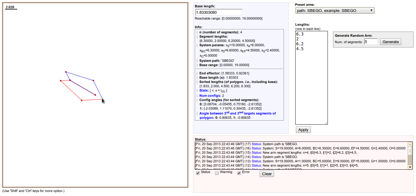
Refer to caption

Figure 19: The Javascript and HTML5 based graphical user interface available at http://hans.math.upenn.edu/~subhrabh/nowiki/robot_arm_JS-HTML5/arm.html .

A simple analysis reveals that the complexity of computing the inverse kinematics is O⁡(n2)O(n^{2}) (equation 15 being computed for q=0,1,⋯,n−1q=0,1,\cdots,n-1). Thus is it possible to implement the algorithm efficiently on a system-independent web-based platform with relatively low computational capabilities. In particular we chose to do a HTML5 + Javascript implementation and made it available on the web at one of the following links:

The interface is highly intuitive (Figure 19). The “preset arms” gives a list of preset arms that can be selected. Mouse position on the workspace on the left indicates the end effector position (holding the ’ctrl’ key lets one move mouse at sub-pixel accuracy), and the program will compute the inverse kinematics to show one or two arm configurations depending on if the state block is of the form [>;∗][>;*] or [<;∗][<;*]. The ‘info’ section displays information about the arm and the current state, and does validating checks on the number of configurations returned and whether or not the two configurations belong to different connected components. The code is optimized to run on a Google chrome browser.

6 Conclusion and Future Direction

Refer to caption
(a) In absence of obstacles there are two connected components of the constrained configuration space at z′z^{\prime}.
Refer to caption
(b) In presence of obstacles there are three connected components of the constrained configuration space at z′z^{\prime}.
Figure 20: An illustration (a low-dimensional analogy – top row does not show actual configuration space) of how having obstacles in the environment can create punctures in ℜ\mathfrak{R}, which in turn can create more connected components in DR−1​(z)D_{R}^{-1}(z), and hence new vital critical points.

The design problem problem addressed in this paper involved sampling exactly one unique configuration for each connected component of the constrained configuration spaces, DR−1​(z)D_{R}^{-1}(z), such that the sampled configurations vary continuously as zz is varied continuously. We motivated the need for solving such a problem from the more practical problem of planning optimal path for the end effector of a robot arm. The said sampling approach would drastically reduce the dimensionality of the search domain in automated manipulation planning using search algorithms like A*. The solution to this problem is made possible by a fundamental theoretical result involving classification of the configuration spaces of planar robot arms.

Moving forward, our next step will be to generalize this technique to the case when the environment contains obstacles. Identifying the vital critical points (Difinition 1) and designing inverse kinematics such that the system pass through the vital critical points will understandably be more difficult in that case, and will require numerical techniques. Figure 20 illustrates the challenges in achieving this.

References

  • [1] Subhrajit Bhattacharya. Topological and Geometric Techniques in Graph-Search Based Robot Planning. PhD thesis, University of Pennsylvania, January 2012.
  • [2] Subhrajit Bhattacharya, Maxim Likhachev, and Vijay Kumar. Topological constraints in search-based robot path planning. Autonomous Robots, pages 1–18, June 2012. DOI: 10.1007/s10514-012-9304-1.
  • [3] S.R. Buss. 3D Computer Graphics: A Mathematical Introduction with OpenGL. Cambridge University Press, 2003.
  • [4] David C Conner, Alfred Rizzi, and Howie Choset. Composition of local potential functions for global robot control and navigation. In Proc. Int’l Conf. on Intelligent Robots and Systems (IROS), pages 3546–3551, 2003.
  • [5] A.A. Goldenberg, B. Benhabib, and R.G. Fenton. A complete generalized solution to the inverse kinematics of robots. Robotics and Automation, IEEE Journal of, 1(1):14–20, 1985.
  • [6] K. Gupta and K. Kazerounian. Improved numerical solutions of inverse kinematics of robots. In Robotics and Automation. Proceedings. 1985 IEEE International Conference on, volume 2, pages 743–748, 1985.
  • [7] Allen Hatcher. Algebraic Topology. Cambridge University Press, 2001.
  • [8] P. E. Hart, N. J. Nilsson, and B. Raphael. A formal basis for the heuristic determination of minimum cost paths. IEEE Transactions on Systems, Science, and Cybernetics, SSC-4(2):100–107, 1968.
  • [9] Eric A. Hansen and Rong Zhou. Anytime heuristic search. Journal of Artificial Intelligence Research (JAIR), 28:267–297, 2007.
  • [10] Beat Jaggi. Configuration spaces of point sets with distance constrains. PhD thesis, Univ. of Bern, 1992. (See the summarized results that appear in the paper “Configuration Spaces of Planar Plygons” by the same author).
  • [11] J. O. Kim and P. K. Khosla. Real-time obstacle avoidance using harmonic potential functions. Robotics and Automation, IEEE Transactions on, 8(3):338–349, Jun 1992.
  • [12] Michael Kapovich and John Millson. On the moduli space of polygons in the euclidean plane. Journal of Differential Geometry, 42:133–164, 1994.
  • [13] A. Kumar, State University of New York at Buffalo. Mechanical, and Aerospace Engineering. Kinesthetic Mapping of RoSS: Robotic Surgical Simulator Using Inverse Kinematics. State University of New York at Buffalo, 2008.
  • [14] Pradeep Khosla and Richard Volpe. Superquadric artificial potentials for obstacle avoidance and approacb. Philadelphia, Apr 1988.
  • [15] G.F. Liu, J.C. Trinkle, and R. J. Milgram. Complete path planning for a planar 2-r manipulator with point obstacles. In Robotics and Automation, 2004. Proceedings. ICRA ’04. 2004 IEEE International Conference on, volume 4, pages 3263–3269 Vol.4, 2004.
  • [16] V. J. Lumelsky. Iterative coordinate transformation procedure for one class of robots. IEEE Transactions on Systems, Man, and Cybernetics.
  • [17] R. Muller-Cajar and R. Mukundan. Triangulation: A new algorithm for inverse kinematics. In Proceedings of Image and Vision Computing, pages 181–186, Hamilton, New Zealand, December 2007.
  • [18] J.W. Milnor. Morse Theory. Annals of mathematics studies. Princeton University Press, 1963.
  • [19] Richard M. Murray, Zexiang Li, and Shankar S. Sastry. A Mathematical Introduction to Robotic Manipulation. CRC Press, 1 edition, March 1994.
  • [20] R. James Milgram and Jeff Trinkle. The geometry of configuration spaces for closed chains in two and three dimensions, 2004.
  • [21] Liviu Nicolaescu. An Invitation to Morse Theory. Springer, 1st edition, 2007.
  • [22] Richard Paul. Robot manipulators: mathematics, programming, and control : the computer control of robot manipulators. MIT Press, Cambridge, MA, 1981.
  • [23] N.E. Steenrod. The Topology of Fibre Bundles. Princeton Mathematical Series. Princeton University Press, 1951.
  • [24] A. Stentz. The focussed D* algorithm for real-time replanning. In Proceedings of the International Joint Conference on Artificial Intelligence (IJCAI), pages 1652–1659, 1995.
  • [25] Payne T.N. and Dauterive F.R. A comparison of total laparoscopic hysterectomy to robotically assisted hysterectomy: surgical outcomes in a community practice. Journal of Minimally Invasive Gynecology, 15(3):286–91, 2008.
  • [26] L.-C.T. Wang and C.C. Chen. A combined optimization method for solving the inverse kinematics problems of mechanical manipulators. Robotics and Automation, IEEE Transactions on, 7(4):489–499, 1991.