AdS-Sliced Flavor Branes and Adding Flavor to the Janus Solution
Abstract
We implement D7 flavor branes in AdS-sliced coordinates on with the ansatz that the brane fluctuates only in the warped () direction in this slicing, which is particularly appropriate for studying the Janus solution. The natural field theory dual in this slicing is super Yang-Mills on two copies of . Branes extending from can end at different locations, giving rise to quarks with piecewise constant mass on each half-space, jumping discontinuously between them. A second class of flavor brane solutions exists in this coordinate system, dubbed “continuous” flavor branes, that extend across the entire range of . We propose that the correct dual interpretation of “disconnected” flavor brane in this ansatz is a quark hypermultiplet with constant mass on one of the AdS4 half-spaces with totally reflecting boundary conditions at the boundary of AdS4; whereas the dual interpretation of a continuous flavor brane has totally transparent boundary conditions. Numerical studies indicate that AdS-sliced D7 flavor branes of both classes exhibit spontaneous chiral symmetry breaking, as non-zero vev persists for solutions of the equation of motion down to zero mass. Continuous flavor branes in this ansatz exhibit many other surprising behaviors: their masses seem to be capped at a modest value near in units of the inverse AdS radius, and there may be a phase transition between continuous branes of different configurations. We also numerically study quark states in Janus. The behavior of mass and vev is similar in Janus, including the existence of chiral symmetry breaking at zero mass, though qualitative features of the phase diagram change (sometimes significantly) as the Janus parameter increases.
I Introduction
Holography and the AdS/CFT correspondence have been exciting fields of study since their discovery late nineties [1, 2, 3]. Matter fields can be added to the gravity side by the well-known prescription of adding a small number, , of “flavor” branes [4]. This breaks half the supersymmetries of the gauge theory. The Janus solution of type IIB supergravity is interesting because locally it is very similar to ordinary AdS space, but the dilaton and 5-form vary in the warped direction in a particular slicing. This situation breaks supersymmetry entirely yet remains stable. The dual gauge theory is most commonly viewed as an “interface” conformal field theory, or ICFT, that is super Yang-Mills theory with a gauge coupling that jumps suddenly at the interface of a domain wall. The jumping coupling is somewhat analogous to filling half the universe with a dielectric medium with a planar interface. This analogy is imprecise in one very important way: the speed of light does not change when crossing the domain wall, as it would if the interface were truly that between two dielectric media.
We expect systems that break supersymmetry to generically also break chiral symmetry as the formation of a condensate is no longer forbidden. Janus provides a novel mechanism for this to occur, since supersymmetry in the dual gauge theory is broken by the jumping of the coupling constant. Chiral symmetry will be broken by the same unusual mechanism. More surprisingly, regular AdS space with flavor branes set up according to a Janus-like ansatz also appears to break chiral symmetry.
II Review of Janus Solution
II.1 Coordinate Systems
We review a variety of coordinate systems for , defined as a hyperboloid in :
| (1) |
We will always work with unit radius. If necessary, the AdS curvature radius can be restored with dimensional analysis.
II.1.1 Global coords
Global coordinates cover the entirety of AdS space. They consist of the following parametrization:
| (2) |
where the are unit vectors on . The coordinate fills the time-like role, and is the warped direction and is bounded . The metric in these coordinates is
| (3) |
II.1.2 Poincaré patch coordinates
Often the most convenient coordinates despite an ugly parametrization:
| (4) | |||
This gives us the metric:
| (5) |
The timelike coordinate is of course , is the warped coordinate bounded , and denotes . Patch coordinates only cover half of the spacetime. If one defines , Poincaré patch coordinates can be recast so that the metric takes on the form:
| (6) |
When it is necessary to distinguish these two coordinate systems we will refer to the coordinates with as “braneworld patch coordinates,” as this is the metric that shows up most naturally when taking the near horizon limit of the spacetime created by a stack of concident D-branes. The coordinate plays the role of a radius or transverse distance from the branes.
A third variation of Poincaré patch coordinates is sometimes useful. Let . Then the metric becomes
| (7) |
II.1.3 AdS-sliced coordinates
First, parameterize , where is an angle in . For the remaining hyperboloid coordinates choose any coordinate system for an AdS space of one lower dimension with variable radius given by . The metric becomes:
| (8) |
We point out a useful identity from [5]. If we take Poincaré patch coordinates on the slices, the full metric is
| (9) |
where is the warped coordinate on the slices and refers to the two non-warped spatial directions on the slices. This can be related to conventional Poincaré patch coordinates by the following transformation:
| (10) | ||||
where is a non-warped direction in conventional Poincaré patch coordinates. For braneworld coordinates, this relation becomes
| (11) |
II.2 The Janus Ansatz
The original Janus solution was an ansatz for a dilaton and 5-form running in the warped direction of a deformed AdS, presented in AdS-sliced coordinates. The deformation alters the warp factor away from and introduces an “angular excess” [5].
When making the Janus ansatz, the warp factor of is promoted from the fixed function to a more general . The dilaton and 5-form are allowed to run in the direction as follows:
| (12) | ||||
| (13) |
where the ’s denote unit volume forms on their respective subspaces. With this ansatz, the supergravity equations of motion reduce to
| (14) |
for the dilaton, where is an integration constant, and
| (15) |
for the warp factor. For more detail see [5, 6]. Equation (15) can be integrated to find the maximum value of , dubbed [5], and the integral can in turn be evaluated in a series expansion for sufficiently small [6, 7]:
| (16) |
It is worth noting that (15) has 4 zeros in , but only two of them are real and only for the choice . So to find a physical solution, one must choose the integration constant within that range and choose initial conditions for so that it equals the largest root of the RHS of (15) at . The second face of Janus arises from analytically continuing the solution to negative values of . This can be implemented by brute force in numerics by taking the square root of equation (15) and multiplying the RHS by .
The main qualitative feature that distinguishes the Janus metric from undeformed AdS is that the boundary occurs at a value of the warped coordinate greater than the so-called “angular excess” [5, 6, 7]. The asymptotic behavior of the warp factor near the boundary is [6], identical at leading order to the behavior AdS. Non-perturbative stability of this solution was shown in [6]. The dual gauge theory was studied in [7]. Many subsequent papers have explored restoring supersymmetry in a Janus framework [8, 9, 10, 11, 12, 13, 14], adding a black hole [15, 16], nesting Janus spacetimes of different dimension [17], and many other variations [18, 19, 20, 21, 22, 23, 24, 25, 26, 27, 28, 29, 30, 31, 32].
III Adding Probe D7 Branes with Janus-slicing
Flavor is traditionally added to AdS/CFT via the prescription of adding probe D7 branes that are spacetime filling in the AdS dimensions, wrap a 3-cycle on the S5 and slip off the pole of the S5 at some finite value of the warped coordinate, thus “ending in thin air” at that location [4]. In the dual theory this corresponds to adding a number of massive hypermultiplets in the fundamental representation of the gauge group. The probe limit means that the number of colors, , is much greater than , so any gravitational backreaction of the D7 branes on the metric can be neglected. As noted in [33], coordinate systems other than Poincaré patch (or braneworld) do not readily admit an interpretation as the near horizon limit of a black D3 brane (or stack of coincident such branes). So we follow the example of [33] and employ the strongest form of the AdS/CFT correspondence. Even if the dual gauge theory cannot be interpreted as the worldvolume theory of a stack of coincident D3 branes, with D7 flavor branes in a coordinate system other than Poincaré patch is a perfectly valid supergravity system and should have a dual gauge theory description, regardless of coordinate system or ansatz for the brane. In [33] flavor branes of various dimension were considered in global coordinates with the ansatz that the branes could fluctuate only in the radial, or , direction. We sill do the same in Janus-sliced coordinates, with the ansatz that the branes can only fluctuate in the direction. Much heuristic intuition can be gained by considering results from flavor branes in Poincaré patch coordinates and replacing , effectively fixing the coordinate to unity. This can serve as a guidepost for certain features, but many details are quite different in the Janus-sliced ansatz. We proceed under the assumption that our description of the dual gauge theory above is correct, exactly parallelling the original D3-D7 system except the natural spacetime for constructing this dual gauge theory consists of two copies of with their boundaries identified. By identifying boundaries, we mean that the boundary conditions for fields in one are related to the boundary conditions in the other, similar to the construction of [34].
We apply the same procedure in Janus-sliced coordinates both with and without the flowing dilaton of Janus itself. The D7 brane extends in the AdS directions and wraps an . The D7 is only allowed to fluctuate in the direction in Janus-sliced coordinates, and it extends from the boundary to some non-zero value of . When the flowing dilaton of Janus is added, we can no longer neglect the factor of the dilaton in the DBI action, and the equation of motion picks up additional terms from the dilaton. Recall that denotes the dilaton field, not an angle. We use Poincaré patch coordinates on the slices with as the warped coordinate of the slices and take and to be the two angles on the S5 that are transverse to the D7 brane. In regular AdS, the DBI action for the Janus-sliced D7 brane has the same form as the usual case, but the warp factor is slightly different:
| (17) |
The DBI action for full Janus can be obtained from (17) by substituting and inserting the factor .
The resulting equation of motion is identical to the general equation of motion for D7 branes presented in [35], but we expand it here to highlight unique features in Janus-sliced coordinates:
| (18) |
Note that arcsine functions do not solve this equation of motion, unlike the original flavor brane ansatz, as can be easily checked by plugging in trial functions. We will turn to numerics to solve this equation of motion in section III.2.
III.1 Asymptotic Expansion in Janus slicing
To examine the near boundary behavior of , we expand our equations of motion about . As in [35], we will begin with the most general possible form for a power series expansion of . We will then substitute this into our EOM, expanded in terms of , and examine the restrictions the EOM place on the coefficients of the expansion. According to the standard AdS/CFT dictionary, in order for the field to properly describe a quark hypermultiplet mass operator in the boundary theory, its near boundary behavior should follow,
| (19) |
with . Thus, the leading behavior should be,
| (20) |
The general expansion for has the form [35]:
| (21) |
We note that this expansion hinges on writing the metric in Fefferman-Graham coordinates [35], and in principle the coefficients of both the expansion of the metric in Fefferman-Graham coordinates and the expansion of bulk fields can be functions of other coordinates than the warped coordinate. The full implementation of Fefferman-Graham coordinates in Janus-sliced coordinates was carried out in [36]; however, for our brane ansatz, the bulk fields cannot vary with any coordinate other than , so we may safely ignore dependence of the coefficients on AdS4 coordinates. The Janus warp factor, , has the same near boundary behavior as the of ordinary , and may be treated as [5, 6]
| (22) |
in the EOM. Furthermore, the dilaton field contributes to the EOM, only through it’s first derivative. Thus we can see from (14) that it may be expanded as
| (23) |
Below, we will keep the notation compact by denoting,
| (24) | |||||
and later expanding these trigonometric functions in their appropriate power series.
Our equation of motion for then takes on the near boundary form:
| (25) |
The explicit dilaton contribution is clearly identifiable, due to the factor of , and can be seen to contribute only at order and higher. Since the leading asymptotic behavior of the warp factor is the same for both the Janus and ordinary AdS solutions, and the explicit dilaton terms in the Janus solution appear beyond the relevant order of , we can conclude that this expansion will proceed identically for both cases. Thus, the asymptotic behavior found below, will apply to both the Janus solution, and the ”sliced branes” in ordinary .
In order to confirm the proper asymptotic behavior for , we must expand the EOM to order . When we explicitly expand (25) in powers of , including all terms relevant up to order , we find,
| (26) |
At first glance, it seems there may be many contributing terms. However, examining the EOM expansion (21) at lower orders in , and looking at both the lowest, and the highest powers of , will reveal some simplifying restrictions:
| (27) | |||||
Recall, that denotes an integer greater than . If we assume that vanishes for and higher, then the second to last term tells us that must also vanish, and so on down the line. If there had been a contribution proportional to , this would have allowed a linear combination of and to vanish as the coefficient of the term. However, this is not the case, as the terms from the portions of the EOM linear in and cancel with one another. As noted in [35], an infinite tower of terms higher order in could exist, but this would invalidate the assumption of the existence of the power series solution. The same argument can also be shown to apply to the various with . Thus, our power series solution for actually has the simpler form,
| (28) |
This mirrors the form found in [35], with the radial coordinate , which vanishes at the boundary, replaced by our which also vanishes at the boundary ( being equal to in the case of ordinary .) Also note that notation for the expansion coefficients varies in the literature. For example, [35] uses where [33] used We chose to minimize confusion between expansion coefficients and angles corresponding to supergravity fields.
Inserting this simpler expansion for into the EOM, we can examine the leading order terms for further restrictions on the remaining coefficients. The first and second order pieces give,
| (29) | |||||
| (30) |
From the lowest order term, it is clear that . The second order contribution reveals that . The vanishing of ensures that there will be no higher powers of contributed by the and terms in the EOM. Thus, the order contribution will be,
| (31) |
The coefficient will thus be undetermined. The coefficients , and will vanish. Then, , when fixed, will determine the value of though the algebraic equation,
| (32) |
This same essential behavior (with a different algebraic equation relating and ) was found in [35]. Insuring that it applies here as well, confirms that our branes – which are embedded differently due to the radial coordinate picked out by the Janus solution – will still properly describe fermion flavors in the boundary theory. This applies equally well in ordinary and Janus spaces.
III.2 Numerics
To solve (18) numerically, we denote by the ending location of the brane and use as initial conditions with to approximate the usual conditions that the brane slip off the north pole with infinite derivative. We present a few sample solutions to the equation of motion in figure 1, the numeric solution is shown in red,and the function is shown in blue for comparison. We plot solutions for 3 different values of on the same axes, for reference.

For large (and thus large mass) the Arcsine function is close to the actual solution, but it gets increasingly inaccurate as decreases. Per the asymptotic expansion, we fit the numeric solutions to , where we have reversed the sign of the difference, , introduced at the beginning of section III.1. The sign reversal is for convenience, so that we plot mostly positive masses, as an overall sign can be introduced in the dual gauge theory by a chiral rotation. For reference, we list the fit parameters for the example solutions shown in Figure 1. For we obtain . For we find fit parameters of 1.40824 and 3.31012 respectively. Finally for we find 3.53835 and 12.2155.
To obtain plots for studying the phase structure of this system, we numerical solve and fit (18) successively from down to in steps of 0.01, then adjust the step size successively to , , and for reasons that will become apparent. Recall that in [4] with arcsine solutions the mass was given by the inverse of the position where the brane ended. For Janus-sliced flavor branes, the relation between mass and is more complicated, given by Figure 2.

For values of near , this has approximately the same shape as , as one might expect from naively extending the relation from [4] with Poincaré patch slicing using , but the relationship is more subtle for lower mass configurations.
We plot vs. in Figure 3, zooming in to give detail in Figure 4. The colors used denote the step size taken in . The blue curve ends at ; the red curve at ; the yellow curve at ; and the green curve (which appears more as a dot) at . The step size for each color is equal to the ending value of . At first, near and again near , it appears that we are making bigger and bigger steps in the plane as we approach . But then the curve appears to stop abruptly at .
There appears to be a kind of limit point in the numerical solutions approaching as . Note, however, that it is impossible to impose “brane ending” boundary conditions at . The boundary condition that causes the term to diverge. For non-zero , the accompanying boundary condition that naturally cancels this divergence when both are implemented as . Unfortunately, when , the coefficients of all the terms in the equation of motion vanish, reducing the equation of motion to . Imposing both boundary conditions simultaneously requires infinite and cannot be solved numerically. If we try a series expansion near , similar to the expansion in [33], promoting the infinitesimal to a small fluctuation, , the action reduces to
| (33) |
The resulting equation of motion is
| (34) |
which does not have an analytic solution except for the trivial one, . The action and lack of a non-trivial solution are consistent with the series expansions in [33] for branes of general dimension that extend in of the AdS dimensions and of the dimensions. Our action for in Janus-sliced coordinates is similar to the action of [33] for , and the critical solution, equation (3.4) of [33], does not exist for the case. This analysis does not rule out the possibility of other solutions not detected by our numerics that would continue the spiral of figure 4 down to ; however, if a non-trivial such solution exists, it does not reach the origin of figure 4 at . This would be extremely puzzling, since this is ordinary AdS space where there is nothing to set a scale or otherwise mark any location other than as special.

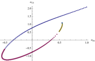
We find evidence of spontaneous chiral symmetry breaking in Figure 4. The mass () reaches zero between and 0.39. Since this occurs with between 0.75398 and 0.784872, we conclude that the dual theory will exhibit spontaneous chiral symmetry breaking as the mass of the quarks is taken zero. This would be expected for Janus proper, but it is surprising to find it in undeformed AdS simply with Janus-sliced flavor branes. Interestingly, this chiral symmetry breaking is not detected by the test proposed in [37, 38], but the geometry in our case is sufficiently different from the backgrounds considered there that this is not too surprising. In particular, there is no central singularity in our geometry so the criteria used in [37] do not apply.
III.3 Asymmetric and Continuous Flavor Branes
Janus-sliced coordinates do not exhibit a horizon, so the possibility exists for a D7 brane to extend across the full range of , from the “right-hand” boundary at , through the “center” at , and out to the “left-hand” boundary at . Indeed, the trivial solution, , obviously exists and gives zero mass, zero vev quarks in the dual theory11 1 We are indebted to A. Karch for these observations.. Furthermore, the flavor branes examined in section III.2 fill only half the spacetime, so quarks in the dual theory would exist in only one of the two spaces. Since the geometry is symmetric under , it is trivial to extend these results by adding a mirror image brane extending from to . This is borne out by numerics: numerically solving (18) from to yields results for and that differ from the values for the corresponding positive by at most . For a given this would give quarks in the dual theory with mass constant across both spaces. However, the two branes are disconnected in the bulk, so there is nothing beyond aesthetics imposing symmetry. The D7 brane in the negative half of space may end at a different distance than the D7 in the positive half of space. The dual theory in such a case would have quark masses that were constant on each but different between the two spaces.
Continuous branes can also exhibit this asymmetry. Generic solutions to (18) for continuous branes exhibit different asymptotic behavior at the two boundaries. If initial conditions are chosen for a continuous brane solution such that the center of AdS, , is a turning point for , then the symmetry of the geometry guarantees that the behavior of will be symmetric at the two boundaries as well. This, too, is borne out by numerics to . For continuous brane solutions, we solve (18) numerically imposing boundary conditions at . For symmetric mass cases, we impose where is a real parameter we step through from -1.57 to +1.57. For a sample solution in this class, see figure 5. For generic cases, we allow the first derivative to be non-zero, giving a two-parameter family of solutions. See figure 6 for a sample solution in this class.


The easiest to understand data on continuous brane solutions come from the symmetric case. We plot vs. for symmetric continuous branes as ranges from -1.57 to +1.57 in steps of 0.005 in figure 7. The plot begins at the origin for , corresponding to the trivial solution. The two spiral arms are symmetric and stem from the fact that changing the sign of in this case simply changes the sign of both fit parameters in the asymptotic solution. The blue curve represents solutions with . The red curve represents and extends out to , with the step size reducing to after we reach , then reducing again to when we reach . The fact that the red curve overlaps the blue so completely is surprising. It certainly indicates that continuous branes cannot produce quarks with arbitrarily large mass. The maximum value of mass in our runs is . The near perfect overlap of the two curves suggests that a phase transition may occur between different types of symmetric, continuous branes: one with positive value of very close to and one with a more modest, negative value of (and vice-versa). The doubling back of the curves also indicates that spontaneous chiral symmetry breaking occurs for continuous flavor branes with where it appears the curve crosses the axis with non-zero intercept, indicating a non-zero vev at zero mass. Note that while this seems a value extremely close to , it occurs well before the region of the possible phase transition.

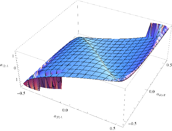
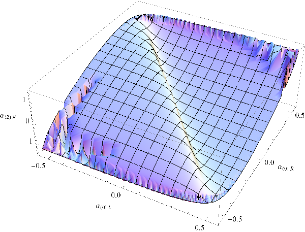
More generic continuous brane solutions require us to fit the asymptotic solution at and separately. We use subscripts “R” and “L,” respectively to denote these different sets of fit parameters. We present our results as a pair of contour plots, figures 8 and 9, treating and as dependent variables that depend on the pair of independent variables . Note the apparent mirror image relationship between the two contour plots.
IV On the Apparent Lack of Phase Transition between Disconnected and Continuous Flavor Branes
The natural expectation is that for low mass continuous branes might be favored while for larger mass disconnected branes might be favored. This does not prove to be the case, however. In figure 10 we overlay the plots from figures 4 and 7, but using blue and red to denote the symmetric brane configurations.
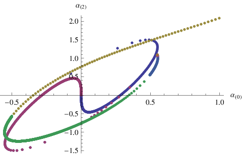
While the curves cross at various points, we do not see the tell-tale merging of the plots that would signal a phase transition. We tried looking for other classes of solutions to fill in the phase diagram, in particular we considered disconnected branes that crossed the center of AdS at and “bubble” branes that pinched off at both a positive and a negative value of and extend through the center. Both seemed to be ruled out by numerics. Attempting to impose boundary conditions (necessary for both classes) while solving for immediately encounters a singularity to the left of when a numeric solution is attempted.
While it remains possible that there exists some class of solutions which we have not discovered, we speculate that the lack of phase transition is because disconnected flavor branes and continuous flavor branes describe incommensurate dual gauge theories. For example, with disconnected branes, even if the masses are chosen to be equal, one need not even choose to use the same number of branes on the left and right sides of AdS. The fact that this option is simply unavailable in the case of continuous branes is the first piece of evidence to suggest the two types of solutions are described by qualitatively different dual gauge theories. A second piece of evidence is the lack of disconnected brane solutions pinching off at . Heuristically, we would have liked to think of the (non-existent) phase transition as occurring when flavor branes on the left and right sides of AdS approached the center and merged. However, in section III.2 we showed that disconnected branes simply cannot “pinch off” at . This was shown both at large scale from the failure of equation (18) to accommodate the “brane pinching off” boundary conditions at and at small scale (small values of ) by the failure of equation (34) to admit non-trivial solutions in the vicinity of . If disconnected branes can never reach or cross , then there is no hope of achieving a phase transition by melding disconnected branes from the left and right halves of AdS in Janus-sliced coordinates.
Since the disconnected branes are confined to one half of the bulk AdS5, we speculate that the dual gauge theories for disconnected and continuous brane solutions differ in the boundary conditions for the quark hypermultiplet fields at the boundary between the two AdS4 halves of the boundary theory. A disconnected brane on the right side of AdS5 seems to naturally correspond to a quark hypermultiplet restricted to the “right” AdS4 in the dual gauge theory with perfectly reflecting boundary conditions at the boundary between the two AdS4 half-spacees. Whereas a continuous flavor brane should correspond to quarks that can freely traverse from the “right” AdS4 to the “left,” corresponding to “transparent” boundary conditions where the leading and sub-leading terms on the two boundary AdS4 spaces match. If this is the correct interpretation of the dual gauge theory, then there clearly cannot be a phase transition as the two scenarios are completely different. However, this hypothesis poses additional puzzles. If continuous flavor branes indeed describe an hypermultiplet with “transparent” boundary conditions between the two AdS4 spaces, there should be no obstacle to large quark mass solutions. Yet the continuous brane solutions do not seem to admit solutions with quark mass larger than about . While it is difficult to see this in the contour plots of figures 8 and 9, it remains true for generic, asymmetric continuous branes as well. The most likely answer is that a second class of continuous flavor brane solutions exists that was not detected by our numerics that admits large mass solutions, although the space of possible alternative explanations is by definition infinite.
V Flavor Branes in Janus
The dynamical factor of the DBI action for such a D7 brane in Janus is
| (35) |
This gives rise to the following equation of motion for :
| (36) |
Qualitatively, turning on the dilaton of Janus does exactly as little as we expect it to thus far: the warp factor is changed slightly, the boundary is pushed out beyond , and the equation of motion for our Janus-sliced flavor branes picks up some extra terms proportional to the derivative of the dilaton field.
Numerically solving (36) with the same “brane pinches off” boundary conditions as in regular AdS for we obtain figure 11.

The left end of each curve corresponds to . Note that the same qualitative shape found for Janus-sliced flavor branes in undeformed AdS is present. As increases, the shape of the curve changes more and more radically, changing convexity and flipping over to the fourth quadrant for .
VI Implications in dual theory
Roughly speaking, the natural choice of conformal factor in AdS slicing gives a dual theory on two copies of joined at their common boundary. If we make this choice for Janus-sliced flavor branes in undeformed AdS, we would expect to find that the quark mass jumps as one crossed the boundary from one AdS4 to the other. After studying Janus-sliced flavor branes in detail, we realize that far more dramatic changes could take place, such as changing the number of flavors. Different choices of conformal factor and thus different coordinate systems in the dual gauge are of course allowed.
Following the general prescription of [2] for constructing the dual gauge theory and the refinements of [39, 40], we obtain the boundary metric by multiplying the AdS metric by , where is any function with a linear zero at the boundary, often dubbed the “conformal factor.” We are specializing to the case of Janus-sliced coordinates in the bulk. For a general bulk scalar field, , of dimension , where generically denotes the “non-warped” directions of AdSd+1 has near boundary behavior given by
| (37) |
It is well known that is the source of the dual operator and is the vev, although the vev is in general a more complicated function of the leading and sub-leading coefficients using the prescription of holographic RG[35]. In the dual theory changing metrics is accomplished with a conformal transformation. In the bulk theory the same is realized by choosing a different conformal factor to regulate the boundary metric. To see the relationships between coefficients with different choices of conformal factor, recall in the bulk the field is a scalar, so each term in the asymptotic expansion must be invariant. If we compare two conformal factors, and , this gives us the relationship between two boundary coefficients of
| (38) | ||||
| (39) |
A similar discussion centered on the operator dual to the dilaton field appears in [7]. Applying this to Janus-sliced flavor branes shows us that if we choose the conformal factor such that the dual theory lives on two copies of AdS4, then the mass of the quarks will be piecewise constant. If we conformally transform to Minkowski space, examining metric (9), we see that the mass becomes a function of in the dual theory:
| (40) |
since the scalar field describing our D7 brane is of dimension 3. Massive quarks in actual Janus will be further complicated by the presence of the operator dual to the dilaton [7], but at leading order this will not effect the position dependence of the mass operator in the dual theory. We postpone more detailed study of the dual theory for future work.
Since the phase diagrams of disconnected brane solutions and continuous brane solutions do not exhibit behavior characteristic of a phase transition, we hypothesize that the two types of brane solution are dual to qualitatively different gauge theories. We propose that continuous brane solutions are dual to an hypermultiplet mass operator that has “transparent” boundary conditions at the shared boundary in AdS4, that is the leading and sub-leading terms should be the same in both half-spaces. Our proposal for the system dual to disconnected flavor branes is that this dual mass operator exhibits totally reflecting boundary conditions: “disconnected” flavor branes on the right AdS4 don’t have any impact on fields in the left AdS4 and vice versa. We think this is the most likely case for several reasons. First, from the gravity side, we could choose to use a different number of flavor branes on each side of AdS5, giving a different number of flavors in the two half-spaces in the dual theory. Second, since the value of the dual operator is determined by the leading order behavior of the gravity state as it approaches the boundary, the coupling of the mass operator from a flavor brane in the right half of AdS5 is literally undefined in the left AdS4 of the dual theory. A brane on the right () does not exist on the left (), so the asymptotic behavior of that state as it approaches is undefined. In the bulk, causality demands that, quite literally, the left brane does not know what the right brane is doing. We see no way to implement this in the dual theory without totally reflecting boundary conditions for the dual quarks in each half-space AdS4. In the dual theory for both flavor brane scenarios, we must impose totally transparent boundary conditions on the gluons as those states are only sensitive to the existence or type of flavor branes through interactions with the quark states.
VII conclusion
We have proposed and analyzed Janus-sliced flavor branes as the appropriate system for studying the addition of flavor to the Janus solution. Janus-sliced coordinates on AdS5 produces a theory most naturally dual to SYM on two copies of AdS4 joined at a common boundary. The main motivation for studying such the system is to look at Janus itself, but our numeric studies have uncovered rich and surprising structure even in undeformed AdS5 without turning on the flowing dilaton of Janus. Janus-sliced coordinates admit possibilities that don’t exist in other coordinate systems: continuous flavor branes that extend from one boundary through the center of AdS out to the other boundary have been studied in global coordinates [33] but are not possible in Poincaré patch, and asymmetric flavor branes that end at different positions on the two “halves” of AdS do not seem to be possible in any other coordinate system.
We have demonstrated that both disconnected and continuous branes exhibit spontaneous chiral symmetry breaking, each possessing a state with non-zero vev at zero mass. Disconnected flavor branes can produce states of arbitrarily large mass, while continuous branes (whether symmetric or not) yield solutions with mass bounded by approximately in units of the inverse AdS radius. This is one of many puzzles associated with the continuous flavor brane solutions, as there seems to be no compelling reason to restrict the mass of quarks in the dual gauge theory, suggesting the existence of yet another class of flavor brane solutions. There may also be a phase transition between continuous flavor branes with values of near and those near , indicated by the overlap in the phase diagram of figure 7. Analysis of the free energies of the brane configurations will be necessary to confirm the existence of such a phase transition.
Since there does not appear to be a phase transition between disconnected flavor branes and connected, we propose that disconnected flavor branes are dual to quark hypermultiplets with piecewise constant mass on AdS4 with totally reflecting boundary conditions at the boundary of each AdS4 half-space, whereas continuous flavor branes are dual to quark hypermultiplets with piecewise constant mass and totally transparent boundary conditions. In both cases, the entire gluon multiplet must have totally transparent boundary conditions. This proposal for differing quark boundary conditions on AdS4 is further supported by gravity-side arguments such as causal disconnection of left and right branes as well as the fact that the number of flavor branes could be chosen to be different on each side.
We have also presented a phase diagram for quarks in Janus proper, using disconnected branes with and three different values of the Janus parameter, . The additional terms in the equation of motion arising from the flowing dilaton make the numerics intrinsically less stable in Janus proper than in undeformed AdS with Janus-sliced coordinates, so we cannot offer as much detail. Qualitatively, we see expected behavior, with large mass when is near , and solutions very similar to undeformed AdS when is small. Large begins to change qualitative features of the phase diagram, pushing the “turnaround point” for the spiral further to the left and reversing the convexity of the curve when is large enough. It will be important for future work to address the mysteries surrounding the continuous flavor brane solutions, determine whether a phase transition exists for “near polar” continuous flavor branes, and study the dual theories we propose in section VI. It is very surprising that simply changing the flavor brane ansatz in this manner results in such a radical change of behavior. It will also be very interesting to study the exact mechanism by which chiral symmetry breaking occurs, both in the dual gauge theory and in the supergravity.
Acknowledgements
ABC and NC would like to thank J. Shock and B. Fadem for helpful conversations. ABC would like to especially thank A. Karch for many patient and detailed conversations about the peculiarities of flavor branes with the Janus-sliced ansatz. The work of NC was partially supported by the Raub Fund. The work of ABC was partially supported by a Faculty Summer Research Grant from the Office of the Provost of Muhlenberg College.
References
- [1] J. M. Maldacena, Adv.Theor.Math.Phys. 2, 231 (1998), hep-th/9711200.
- [2] E. Witten, Adv.Theor.Math.Phys. 2, 253 (1998), hep-th/9802150.
- [3] S. Gubser, I. R. Klebanov, and A. M. Polyakov, Phys.Lett. B428, 105 (1998), hep-th/9802109.
- [4] A. Karch and E. Katz, JHEP 0206, 043 (2002), hep-th/0205236.
- [5] D. Bak, M. Gutperle, and S. Hirano, JHEP 0305, 072 (2003), hep-th/0304129.
- [6] D. Freedman, C. Nunez, M. Schnabl, and K. Skenderis, Phys.Rev. D69, 104027 (2004), hep-th/0312055.
- [7] A. Clark, D. Freedman, A. Karch, and M. Schnabl, Phys.Rev. D71, 066003 (2005), hep-th/0407073.
- [8] A. Clark and A. Karch, JHEP 0510, 094 (2005), hep-th/0506265.
- [9] E. D’Hoker, J. Estes, and M. Gutperle, Nucl.Phys. B757, 79 (2006), hep-th/0603012.
- [10] E. D’Hoker, J. Estes, and M. Gutperle, Nucl.Phys. B753, 16 (2006), hep-th/0603013.
- [11] E. D’Hoker, J. Estes, and M. Gutperle, JHEP 0706, 021 (2007), 0705.0022.
- [12] M.-W. Suh, JHEP 1109, 064 (2011), 1107.2796.
- [13] C. Kim, E. Koh, and K.-M. Lee, Phys.Rev. D79, 126013 (2009), 0901.0506.
- [14] E. D’Hoker, J. Estes, and M. Gutperle, JHEP 0706, 022 (2007), 0705.0024.
- [15] D. Bak, M. Gutperle, and S. Hirano, JHEP 0702, 068 (2007), hep-th/0701108.
- [16] D. Bak, M. Gutperle, and R. A. Janik, JHEP 1110, 056 (2011), 1109.2736.
- [17] S. Hirano, JHEP 0605, 031 (2006), hep-th/0603110.
- [18] C. Bachas and J. Estes, JHEP 1106, 005 (2011), 1103.2800.
- [19] T. Nishioka and H. Tanaka, JHEP 1102, 023 (2011), 1010.6075.
- [20] M. Chiodaroli, M. Gutperle, and L.-Y. Hung, JHEP 1009, 082 (2010), 1005.4433.
- [21] M. Chiodaroli, E. D’Hoker, and M. Gutperle, JHEP 1003, 060 (2010), 0912.4679.
- [22] M. Chiodaroli, M. Gutperle, and D. Krym, JHEP 1002, 066 (2010), 0910.0466.
- [23] E. D’Hoker, J. Estes, M. Gutperle, and D. Krym, JHEP 0909, 067 (2009), 0906.0596.
- [24] E. D’Hoker, J. Estes, M. Gutperle, and D. Krym, JHEP 0906, 018 (2009), 0904.3313.
- [25] S. Ryang, JHEP 0905, 009 (2009), 0903.4500.
- [26] B. Chen, Z.-b. Xu, and C.-y. Liu, JHEP 0902, 036 (2009), 0811.3482.
- [27] Y. Honma, S. Iso, Y. Sumitomo, and S. Zhang, Phys.Rev. D78, 025027 (2008), 0805.1895.
- [28] D. Gaiotto and E. Witten, JHEP 1006, 097 (2010), 0804.2907.
- [29] C. Kim, E. Koh, and K.-M. Lee, JHEP 0806, 040 (2008), 0802.2143.
- [30] T. Azeyanagi, A. Karch, T. Takayanagi, and E. G. Thompson, JHEP 0803, 054 (2008), 0712.1850.
- [31] D. Bak, Phys.Rev. D75, 026003 (2007), hep-th/0603080.
- [32] J. Sonner and P. K. Townsend, Class.Quant.Grav. 23, 441 (2006), hep-th/0510115.
- [33] A. Karch, A. O’Bannon, and L. G. Yaffe, JHEP 0909, 042 (2009), 0906.4959.
- [34] O. Aharony, A. B. Clark, and A. Karch, Phys.Rev. D74, 086006 (2006), hep-th/0608089.
- [35] A. Karch, A. O’Bannon, and K. Skenderis, JHEP 0604, 015 (2006), hep-th/0512125.
- [36] I. Papadimitriou and K. Skenderis, JHEP 0410, 075 (2004), hep-th/0407071.
- [37] N. Evans, J. P. Shock, and T. Waterson, JHEP 0503, 005 (2005), hep-th/0502091.
- [38] N. J. Evans and J. P. Shock, Phys.Rev. D70, 046002 (2004), hep-th/0403279.
- [39] V. Balasubramanian, P. Kraus, and A. E. Lawrence, Phys.Rev. D59, 046003 (1999), hep-th/9805171.
- [40] V. Balasubramanian, P. Kraus, A. E. Lawrence, and S. P. Trivedi, Phys.Rev. D59, 104021 (1999), hep-th/9808017.