On the frequencies of patterns of rises and falls

Consider a data series, such as e.g. the daily temperature at a given weather station over one year. The most obvious features of such a data series are its rises and falls. Physics and other branches of science provide plenty of examples of datasets where the statistics of geometrical features, such as maxima and minima, or rises and falls, is of central interest. One example from statistical physics is provided by energy landscapes, which are ubiquitously present in theoretical studies of systems ranging from glasses to proteins [1].

In this work we investigate the probability of observing a given pattern of $n$ rises and falls in a random stationary data series. This question has hardly been addressed so far in the physics literature, in strong contrast with the statistics of extreme values, which has recently attracted a lot of attention in many areas, including random walks, disordered systems, growth processes and random matrices [2, 3, 4, 5, 6, 7].

The setting of the present work is meant to provide a null model, to which real data could be compared. A first attempt has been made recently in this direction, with the analysis of microarray time series data in genetics [8]. We model the data series as a sequence of $n+1$ i.i.d. (independent and identically distributed) random numbers $x_{i}$ drawn from a continuous distribution. As these random numbers will only occur in inequalities, their distribution can be chosen to be uniform on the unit interval. This probabilistic approach is exposed in Section 3. An equivalent combinatorial approach (see Section 4) is obtained by coarse-graining the random numbers according to the permutation which brings them to an increasing order. We are thus led to model the data as a uniformly chosen random permutation on $n+1$ objects. This line of thought dates back to the pioneering study of alternating permutations by André [9, 10], and it has since then been addressed regularly in the mathematical literature [11, 12, 13, 14, 15, 16, 17, 18, 19, 20, 21, 22, 23, 24, 25, 26, 27, 28] (this list of references is not meant to be exhaustive). To close, let us mention that the combinatorial approach to our problem pertains to the more general topic of patterns in permutations, which has been for long an active area of discrete mathematics [29, 30, 31].

Our goal is to provide a comprehensive and self-contained exposition of the calculation of the frequencies of patterns of rises and falls in a random stationary data series. We aim at using a language accessible to a broad readership in statistical physics. Let us give the detailed setup of this paper and summarize our findings.

The probabilistic and combinatorial approaches, respectively exposed in Sections 3 and 4, provide two equivalent definitions of the probability $P_{n}({\varepsilon_{1}\dots\varepsilon_{n}})$ of observing a given pattern ${\varepsilon_{1}\dots\varepsilon_{n}}$ of $n$ rises and falls. The equivalence between both approaches has already been underlined in several works [8, 21, 23, 24, 25, 27, 28]. It will become clear in the following that each approach has its advantages: the probabilistic one is more suitable for analytical investigations, while the combinatorial one results in a simple recursive structure, lending itself to exact numerical calculations.

In Section 5 we show explicit results for small patterns (up to $n=4$). We then present a heuristic analysis demonstrating that the probability of observing a pattern is essentially determined by its excursion, as long as its length is modest.

In the remainder of the paper, the emphasis is on asymptotic properties in the regime of most interest, at least from the viewpoint of statistical physics, i.e., where the length $n$ of the pattern is large. In this regime the probability $P_{n}({\varepsilon_{1}\dots\varepsilon_{n}})$ typically falls off exponentially as

The decay rate $\alpha$ will be our central object of interest. This quantity can be viewed as the embedding entropy of the binary pattern ${\varepsilon_{1}\dots\varepsilon_{n}}$, i.e., the entropic cost per unit length for embedding this pattern into a sequence of i.i.d. random numbers. It is worth noticing that the above definition is entirely parameter-free. If all the $2^{n}$ patterns of length $n$ had equal probabilities $P_{n}=2^{-n}$, the rate would be constant and equal to $\alpha=\ln 2$. The observed wide range of possible values of the rate $\alpha$, from $\alpha_{\rm min}=\ln(\pi/2)=0.451582\dots$ to infinity, testifies the richness of the problem.

Periodic patterns are investigated in sections 6, 7, and 8. As already mentioned, the subject is an old classic of discrete mathematics. Our comprehensive approach allows us to recover many known results by more elementary means, and often to express them in simpler terms. Section 6 is a self-contained presentation of some of the beauties of the historical example of alternating patterns, for which the rate $\alpha$ assumes its minimal value $\alpha_{\rm min}$. Section 7 deals with the family of $p$-alternating periodic patterns, whose motif (unit cell) consists of $p-1$ rises followed by a fall. The rate reads $\alpha=\ln z_{0}$, where $z_{0}$ is the smallest real positive zero of a generalized trigonometric function. In Section 8 we show how the rate $\alpha$ can be evaluated exactly for an arbitrary periodic pattern, with any period $p\geq 2$: $z_{0}$ is now the smallest zero of a determinant of generalized hyperbolic or trigonometric functions, whose size is at most $p/2$. Many examples are treated explicitly.

The rest of the paper covers entirely novel areas. Sections 9 and 10 serve as an intermezzo. In Section 9 we deal with examples of aperiodic patterns which are built from three classical self-similar sequences: Fibonacci, Thue-Morse, and Rudin-Shapiro. The probabilities $P_{n}$ exhibit an exponential decay, characterized by a well-defined rate $\alpha$, modulated by a fractal amplitude which reflects the self-similarity of the underlying sequence. Section 10 is devoted to chirping patterns, consisting mostly of rises, whereas falls are more and more scarce (or vice versa). In this case the probabilities $P_{n}$ are found to decay super-exponentially. Their asymptotic form is predicted more precisely in the situation of most interest where the density of falls follows a power law.

Section 11 is devoted to the heart of the problem, namely the statistics of the probabilities $P_{n}$ if patterns are chosen in various ensembles of random patterns of fixed length $n$. The uniform ensemble, where all patterns are considered with equal weights, is studied thoroughly. The probabilities $P_{n}$ of generic patterns have the typical rate $\alpha_{0}=0.806361\dots$ The latter number can be interpreted as a Lyapunov exponent. The whole set of probabilities $P_{n}$ is shown to obey multifractal statistics, with a non-trivial spectrum of multifractal dimensions $f(\alpha)$, increasing from $f(\alpha_{\rm min})=0$ to $f(\alpha_{0})=1$. Other ensembles of random patterns of fixed length $n$, namely the ensemble at fixed concentration $c$ of rises and a symmetric Markovian ensemble defined by a persistence probability $r$, are also investigated. The probabilities $P_{n}$ now generically decay according to effective typical rates $\beta(c)$ and $\gamma(r)$, which depend continuously on the ensemble parameters.

Two appendices are respectively devoted to the explicit correspondence between the combinatorial and probabilistic approaches (A) and to generalized hyperbolic and trigonometric functions (B).

The probabilistic approach goes as follows. The data series is modeled by a sequence of $n+1$ i.i.d. random numbers $x_{i}$ ($i=0,\dots,n$), drawn from the uniform distribution on the unit interval $[0,\,1]$. This sequence of random numbers yields a pattern ${\varepsilon_{1}\dots\varepsilon_{n}}$ of $n$ rises and falls defined as follows. For $i=1,\dots,n$:

Let us start with the example shown in Figure 1. This configuration obeys the inequalities $x_{0}<x_{1}<x_{2}>x_{3}$, and therefore yields the pattern $++-$. The probability of observing this pattern reads

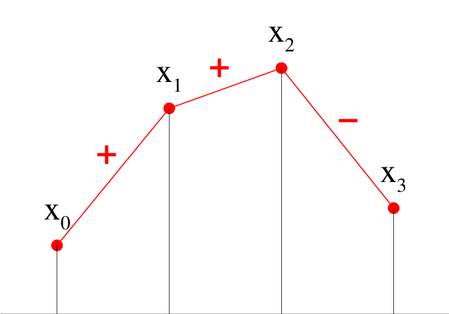
Let us now turn to the general case. The probability of an arbitrary pattern ${\varepsilon_{1}\dots\varepsilon_{n}}$ can be calculated recursively by conditioning on $x_{n}$. Let $f_{n}(x)\,{\rm d}x$ be the probability that the sequence $x_{0},\dots,x_{n}$ yields the pattern ${\varepsilon_{1}\dots\varepsilon_{n}}$ and that $x<x_{n}<x+{\rm d}x$. The conditional densities $f_{n}(x)$ obey the recursion relations:

with the initial condition $f_{0}(x)=1$. It follows that $f_{n}(x)$ is a polynomial in $x$ with degree $n$. We have

This recursive scheme has already been described in [23, 24, 28]. For the example of Figure 1, we get

The second of the nested integral expressions (3) is thus recovered.

In the combinatorial approach the data series is modeled by a permutation ${\sigma}$, chosen uniformly among the $(n+1)!$ permutations on $n+1$ objects labelled $i=0,\dots,n$. Such a permutation yields a pattern ${\varepsilon_{1}\dots\varepsilon_{n}}$, defined as follows. For $i=1,\dots,n$:

The pattern ${\varepsilon_{1}\dots\varepsilon_{n}}$ is said to be the up-down signature of the permutation ${\sigma}$.

Let us again consider the example shown in Figure 1. We have

Let us coarse-grain this configuration of random numbers by representing it as a permutation ${\sigma}$. The rule is that the inverse permutation ${\sigma}^{-1}$ gives the order of indices in the inequalities (8). We thus have ${\sigma}^{-1}=(0312)$,¹¹ 1 We use the one-line notation ${\sigma}=({\sigma}_{0}{\sigma}_{1}\dots{\sigma}_{n})$. and so ${\sigma}=(0231)$, which indeed yields the pattern $++-$.

How many permutations on 4 objects yield the pattern $++-$ ? This simple question can be solved by inspection. There are 3 such permutations: (0132), (0231) and (1230). We thus recover the result (see (3))

It is indeed clear that all the $4!$ permutations on 4 objects are equally probable. This observation demonstrates (on an example) the equivalence between the probabilistic approach of Section 3 and the present combinatorial one (see [8, 21, 23, 24, 25, 27, 28]).

Let us now turn to the general case. The number $A_{n}({\varepsilon_{1}\dots\varepsilon_{n}})$ of permutations on $n+1$ objects yielding a given pattern ${\varepsilon_{1}\dots\varepsilon_{n}}$ of $n$ rises and falls can be calculated by an efficient recursive scheme, which seems to have been discovered several times independently [14, 19, 20]. The gist of the method is similar to that of the probabilistic approach. It consists in conditioning the permutation ${\sigma}$ on its last entry ${\sigma}_{n}$, and to relate the patterns formed by $n+1$ and $n$ objects. Let $a_{n,j}$ be the number of permutations which yield the pattern ${\varepsilon_{1}\dots\varepsilon_{n}}$ and have ${\sigma}_{n}=j$. These numbers can be shown to obey the recursion relations

with the initial condition $a_{0,0}=1$. Arrows indicate the order in which the recursion relations have to be used. We thus build a triangular array of integers:

At the $n$th row, all arrows go from left to right if $\varepsilon_{n}=+$, and from right to left if $\varepsilon_{n}=-$ (see (26) for an example).

The requested numbers of permutations

can also be read off from the array $a_{n,j}$. We have indeed

Finally, the probability that a random permutation on $n+1$ objects yields the pattern ${\varepsilon_{1}\dots\varepsilon_{n}}$ reads

To close, let us write down explicitly the correspondence between the probabilistic and combinatorial approaches. For a given pattern ${\varepsilon_{1}\dots\varepsilon_{n}}$, the probabilistic approach involves the $n$th degree polynomial $f_{n}(x)$, which has $n+1$ coefficients, while the combinatorial one involves the $n+1$ integers $a_{n,j}$. These two sets of numbers carry the same information. The precise correspondence, to be established in A, is summarized by the formula

Table 1 presents explicit results for patterns of length up to $n=4$. For each length $n$, the $2^{n}$ patterns are listed in lexicographical order. For each pattern ${\varepsilon_{1}\dots\varepsilon_{n}}$, the Table gives the number $A_{n}({\varepsilon_{1}\dots\varepsilon_{n}})$ of permutations yielding that pattern and the corresponding probability $P_{n}({\varepsilon_{1}\dots\varepsilon_{n}})$, obtained by means of (10), (12), and (14). These numbers exhibit the expected up-down and left-right symmetries. They also manifest a scatter which increases rapidly with $n$.

The data shown in Table 1 can be analyzed in the following heuristic way. The probability $P_{n}({\varepsilon_{1}\dots\varepsilon_{n}})$ can be expected to be strongly penalized for patterns which make large excursions in the vertical direction. This notion can be formalized as follows. To the pattern ${\varepsilon_{1}\dots\varepsilon_{n}}$ we associate a random walk with steps $\varepsilon_{i}$, i.e.,

with $h_{0}=0$, and we define the excursion of the pattern as the variance of the position of that walk:

For a fixed length $n$, the patterns with the largest excursion are the two straight ones, consisting only of rises, or of falls, for which we have

These patterns also have the smallest probabilities. Consider for definiteness the rising pattern (${\varepsilon_{1}\dots\varepsilon_{n}}=+\cdots+$). The probabilistic approach yields

while the combinatorial approach yields

where the Kronecker symbol $\delta_{n,j}$ equals 1 if $j=n$ and 0 else. There is indeed one single permutation yielding the rising pattern, namely the identity (${\sigma}_{j}=j$ for all $j$). Both approaches consistently give

This factorial decay corresponds to a logarithmically divergent rate

and so $\alpha_{\rm max}=\infty$.

The patterns with the smallest excursion are the two alternating ones, $+-+-\cdots$ and $-+-+\cdots$, for which we have

These patterns, which will be investigated thoroughly in Section 6, are also known to have the largest probabilities [13, 19]. The corresponding rate $\alpha$ takes its minimum value $\alpha_{\rm min}=\ln(\pi/2)$ (see (41)).

More generally, we observe (see Figure 2) that the probability $P_{n}$ and the excursion $\Delta_{n}^{2}$ are strongly anti-correlated.

The observed negative correlation however progressively fades away as the length of patterns is increased. Figure 3 shows a plot of exact numerical data²² 2 Throughout the following, the expression exact numerical data refers to results obtained by iterating numerically the combinatorial recursion (10). for the absolute correlation coefficient $|c_{n}|$ between $\Delta_{n}^{2}$ and $\ln P_{n}$ for lengths up to $n=30$. The fit to the data suggests that this coefficient falls off asymptotically as $n^{-1/2}$.

A statistical analysis of the probabilities $P_{n}$ adapted to their behavior for large lengths $n$, based on the multifractal formalism, will be presented in Section 11.1.

This Section is devoted to the historical example of alternating patterns $+-+-+-\cdots$, studied long ago by André in the framework of alternating permutations [9, 10].

We pursue our investigation with the periodic patterns with any period $p\geq 2$ whose motif (unit cell) consists of $p-1$ rises followed by one single fall. In other words, we have $\varepsilon_{kp+q}=+$ for $q=1,\dots,p-1$ and $\varepsilon_{kp}=-$. These $p$-alternating patterns have been investigated in [15, 16, 24, 26, 28].

We now turn to the analysis of an arbitrary periodic pattern with period $p\geq 2$, whose motif consists of $p-\nu$ rises and $\nu$ falls. If $\nu=0$ or $\nu=p$, the pattern is one of the straight ones discussed in Section 5. Without loss of generality, we can assume $1\leq\nu\leq p/2$ (otherwise exchange the roles of rises and falls). Finally, as we are chiefly interested in the rate $\alpha$, we can use cyclic invariance (see point (ii) below (48)) to ensure that the motif ends with a fall.

References

- [1] D. J. Wales, Energy Landscapes, Cambridge University Press, Cambridge, 2003.
- [2] C. A. Tracy, H. Widom, Level-spacing distributions and the Airy kernel, Commun. Math. Phys. 159 (1994) 151–174.
- [3] C. A. Tracy, H. Widom, On orthogonal and symplectic matrix ensembles, Commun. Math. Phys. 177 (1996) 727–754.
- [4] P. Le Doussal, C. Monthus, Exact solutions for the statistics of extrema of some random 1D landscapes, application to the equilibrium and the dynamics of the toy model, Physica A 317 (2003) 140–198.
- [5] S. N. Majumdar, A. Comtet, Exact maximal height distribution of fluctuating interfaces, Phys. Rev. Lett. 92 (2004) 225501.
- [6] G. Biroli, J. P. Bouchaud, M. Potters, On the top eigenvalue of heavy-tailed random matrices, Europhys. Lett. 78 (2007) 10001.
- [7] D. S. Dean, S. N. Majumdar, Extreme value statistics of eigenvalues of Gaussian random matrices, Phys. Rev. E 77 (2008) 041108.
- [8] T. M. A. Fink, K. Willbrand, F. C. S. Brown, 1-D random landscapes and non-random data series, Europhys. Lett. 79 (2007) 38006.
- [9] D. André, Développements de et , C. R. Acad. Sci. (Paris) 88 (1879) 965–967.
- [10] D. André, Sur les permutations alternées, J. Math. Pures Appl. (Série 3) 7 (1881) 167–184.
- [11] P. A. MacMahon, Combinatory Analysis, Cambridge University Press, Cambridge, 1915-16.
- [12] R. C. Entringer, A combinatorial interpretation of the Euler and Bernoulli numbers, Nieuw. Arch. Wisk. 14 (1966) 241–246.
- [13] I. Niven, A combinatorial problem on finite sequences, Nieuw. Arch. Wisk. 16 (1968) 116–123.
- [14] N. G. de Bruijn, Permutations with given ups and downs, Nieuw. Arch. Wisk. 18 (1970) 61–65.
- [15] L. Carlitz, Permutations with prescribed pattern, Math. Nachr. 58 (1973) 31–53.
- [16] L. Carlitz, R. Scoville, Enumeration of rises and falls by position, Discrete Math. 5 (1973) 45–59.
- [17] M. Abramson, A note on permutations with fixed pattern, J. Combin. Theory (Series A) 19 (1975) 237–239.
- [18] H. O. Foulkes, Enumeration of permutations with prescribed up-down and inversion sequences, Discrete Math. 15 (1976) 235–252.
- [19] G. Viennot, Permutations ayant une forme donnée, Discrete Math. 26 (1979) 279–284.
- [20] M. D. Atkinson, On zigzag permutations and comparisons of adjacent elements, Information Processing Lett. 21 (1985) 187–189.
- [21] C. L. Mallows, L. A. Shepp, Enumerating pairs of permutations with the same up-down form, Discrete Math. 54 (1985) 301–311.
- [22] D. R. van Baronaigien, F. Ruskey, Generating permutations with given ups and downs, Discrete Applied Math. 36 (1992) 57–65.
- [23] G. G. Szpiro, The number of permutations with a given signature, and the expectations of their elements, Discrete Math. 226 (2001) 423–430.
- [24] E. A. Bender, W. J. Helton, L. B. Richmond, Asymptotics of permutations with nearly periodic patterns of rises and falls, Electron. J. Combin. 10 (2003) R40.
- [25] F. C. S. Brown, T. M. A. Fink, K. Willbrand, On arithmetic and asymptotic properties of up-down numbers, Discrete Math. 307 (2007) 1722–1736.
- [26]
A. Mendes, J. B. Remmel,
Generating
functions from symmetric functions.
URL http://www.math.ucsd.edu/$\sim$remmel/files/Monograph.p%s - [27] N. Basset, Counting and generating permutations using timed languages, preprint hal-00820373 (October 2013).
- [28] P. Marchal, Permutations with a prescribed descent set, preprint hal-00944244 (February 2014).
- [29] M. Bóna, Combinatorics of Permutations (Discrete Mathematics and Its Applications), CRC Press, Boca Raton, Fla., 2004.
- [30] S. Linton, N. Ruskuc, V. Vatter, Permutation Patterns, London Mathematical Society Lecture Note Series, Vol. 376, Cambridge University Press, Cambridge, 2010.
- [31] S. Kitaev, Patterns in Permutations and Words, Springer, Berlin, 2011.
- [32] J. Millar, N. J. A. Sloane, N. E. Young, A new operation on sequences: The boustrophedon transform, J. Combin. Theory (Series A) 76 (1996) 44–54.
- [33] L. Seidel, Über eine einfache Entstehungsweise der Bernoulli’schen Zahlen und einiger verwandten Reihen, Sitzungsber. Münch. Akad. 4 (1877) 157–187.
- [34]
OEIS, The On-Line Encyclopedia of Integer
Sequences.
URL http://oeis.org - [35] B. Derrida, E. Gardner, Metastable states of a spin glass chain at 0 temperature, J. Phys. (Paris) 47 (1986) 959–965.
- [36] D. J. Leeming, R. A. MacLeod, Some properties of generalized Euler numbers, Canad. J. Math. 33 (1981) 606–617.
- [37] D. J. Leeming, R. A. MacLeod, Generalized Euler number sequences: asymptotic estimates and congruences, Canad. J. Math. 35 (1983) 526–546.
- [38] M. Queffélec, Substitution Dynamical Systems. Spectral Analysis, Springer, Berlin, 1987.
- [39] E. L. Albuquerque, M. G. Cottam, Theory of elementary excitations in quasiperiodic structures, Phys. Rep. 376 (2003) 225–337.
- [40] D. Shechtman, I. Blech, D. Gratias, J. W. Cahn, Metallic phase with long-range orientational order and no translational symmetry, Phys. Rev. Lett. 53 (1984) 1951–1953.
- [41] G. Paladin, A. Vulpiani, Anomalous scaling laws in multifractal objects, Phys. Rep. 156 (1987) 147–225.
- [42] J. Feder, Fractals, Plenum, New York, 1988.
- [43] D. Harte, Multifractals: Theory and Applications, CRC Press, Boca Raton, Fla., 2001.
- [44] L. Carlitz, Some arithmetic properties of the Olivier functions, Math. Ann. 128 (1954) 412–419.
- [45] L. Olivier, Bemerkungen über eine Art von Funktionen, welche ähnliche Eigenschaften haben, wie die Cosinus und Sinus, J. Reine Angew. Math. 2 (1827) 243–251.
- [46]
E. W. Weisstein, Generalized hyperbolic functions,
from MathWorld–A Wolfram Web Resource.
URL http://mathworld.wolfram.com/\GeneralizedHyperbolicFunctions.html