跳到论文正文
W Papers独立论文阅读器 arXiv:1309.7664 论文正文 计算阅读时间 · 0%
引用这篇论文根据当前论文元数据生成,正式投稿前建议核对。


License: arXiv.org perpetual non-exclusive license
arXiv:1309.7664v1 [math-ph] 29 Sep 2013

Imaging strong localized scatterers with sparsity promoting optimization

This version: August 1, 2013. M. M. and G. P. were supported by AFOSR grant FA9550-11-1-0266.
Anwei Chai ††thanks: anwei@math.stanford.edu Affiliation: Department of Mathematics, Stanford University, California 94305, USA    Miguel Moscoso ††thanks: moscoso@math.uc3m.es Affiliation: Gregorio Millán Institute, Universidad Carlos III de Madrid, Madrid 28911, Spain    George Papanicolaou ††thanks: papanico@math.stanford.edu Affiliation: Department of Mathematics, Stanford University, California 94305, USA
Abstract

We study active array imaging of small but strong scatterers in homogeneous media when multiple scattering between them is important. We use the Foldy-Lax equations to model wave propagation with multiple scattering when the scatterers are small relative to the wavelength. In active array imaging we seek to locate the positions and reflectivities of the scatterers, that is, to determine the support of the reflectivity vector and the values of its nonzero elements from echoes recorded on the array. This is a nonlinear inverse problem because of the multiple scattering. We show in this paper how to avoid the nonlinearity and form images non-iteratively through a two-step process which involves ℓ1\ell_{1} norm minimization. However, under certain illuminations imaging may be affected by screening, where some scatterers are obscured by multiple scattering. This problem can be mitigated by using multiple and diverse illuminations. In this case, we determine solution vectors that have a common support. The uniqueness and stability of the support of the reflectivity vector obtained with single or multiple illuminations are analyzed, showing that the errors are proportional to the amount of noise in the data with a proportionality factor dependent on the sparsity of the solution and the mutual coherence of the sensing matrix, which is determined by the geometry of the imaging array. Finally, to filter out noise and improve the resolution of the images, we propose an approach that combines optimal illuminations using the singular value decomposition of the response matrix together with sparsity promoting optimization jointly for all illuminations. This work is an extension of our previous paper [5] on imaging using optimization techniques where we now account for multiple scattering effects.

Keywords. array imaging, joint sparsity, multiple scattering, Foldy-Lax equations

1 Introduction

Active array imaging when multiple scattering between the scatterers is important is challenging because it is a nonlinear inverse problem. In most applications, for example, in seismic imaging, ultrasonic non-destructive testing, synthetic aperture radar, etc., the imaging methods that are used ignore multiple scattering and deal with a linear inverse problem. This may result in some loss of resolution, especially if the imaging setup provides only partial information with, for example, a limited frequency range, limited illuminations or small arrays relative to the distance from the scatterers. In this paper, we study active array imaging at only one frequency and with single and multiple illuminations. The arrays considered are not small and could surround the scatterers. We consider the full nonlinear inverse problem when multiple scattering is included but limit the analysis to the case of imaging when the scatterers are small compared to the wavelength so that the Foldy-Lax approximation [12, 15, 16, 1, 19] can be used. Given the array data, we formulate imaging as an underdetermined optimization problem with nonlinear constraints. It is underdetermined because the set of possible locations of the scatterers in the image regions we consider here is much larger than the array data set, as is often the case.

In this paper, we formulate the nonlinear optimization problem for imaging in two steps. In the first step, we treat the scatterers as equivalent sources of unknown locations whose strengths are also unknown but are related in a known way to the illumination, to the multiple scattering and to the underlying unknown reflectivities of the scatterers. Under specific, if somewhat conservative, hypotheses about the array imaging setup and the measurement noise level, we show that the location of the sources, that is, the scatterers, can be recovered exactly in the first step. This is because we employ an ℓ1\ell_{1} minimization method that recovers the support of sparse solutions exactly. In the second step, once the location of the scatterers is fixed, their true reflectivities can be recovered using the known relationship to the source strengths obtained in step one. This is an explicit relation that comes from the Foldy-Lax equations, given the scatterer locations. The key to this two-step approach is the possibility of recovering exactly the locations of the scatterers in the first step. This effectively linearizes what is a nonlinear inverse problem. Our theoretical analysis is mainly based on the work by Tropp [24]. We give sufficient conditions on the imaging setup under which we can expect perfect reconstructions without noise, and conditions under which these reconstructions are stable when the data is contaminated with additive noise.

We note that the two-step imaging method we have described is applied at first to array data from a single illumination, in §3. However, because of the screening effects, not all scatterers can be recovered from data generated by a single illumination, in general. Moreover, using a single illumination with array imaging configurations often used in practice is not robust when data is contaminated with noise. These issues can be handled by applying the same two-step imaging method to data from multiple illuminations. For this case, a matrix version of the ℓ1\ell_{1} minimization method is described and analyzed in §4.

When we have access to the full array response matrix, that is, when we have data for a full set of linearly independent illumination vectors, it is possible to image using its singular value decomposition (SVD). This is done in [14, 8, 18] where the authors show that, despite of the nonlinearity of the mapping from the reflectivities of the scatterers to the data received on the array, one can form an image and find the locations of the individual point scatterers by beamforming with the significant singular vectors. This is the MUSIC (MUltiple SIgnal Classification) method, which is essentially the same as beamforming or migration using the significant singular vectors as illuminations. These illumination vectors are optimal in the sense that they result in array data with maximal power, which is proportional to the associated singular values.

We also use optimal illuminations in the ℓ1\ell_{1} based minimization approach we introduce here. This increases the efficiency of the data collection process and lowers the impact of the noise in the data, as we show with numerical simulations in §6. This is so even when only a few optimal illuminations are used. We used optimal illuminations in [5] for a proposed hybrid ℓ1\ell_{1} method in the context of array imaging when multiple scattering is negligible. The hybrid ℓ1\ell_{1} method not only uses the optimal illumination but also projects the data into appropriate subspaces. This last step cannot be carried out when multiple scattering is important because after projection the sensing matrix contains unknown factors related to the multiple scattering.

Finally, the performance of the imaging method we propose depend on the mutual coherence of the sensing matrix, defined in §3. We, therefore, carry out an analysis of the mutual coherence of the sensing matrix upon different imaging configurations, with planar and spherical arrays, in §5. We show that spherical arrays give images with better resolutions and smaller upper bound of the corresponding sensing matrix than planar arrays.

We note that the formulation for imaging with non-negligible multiple scattering can also be combined with the optimization approach for imaging problems with intensity only measurements, which is studied by the authors in [4].

The organization of the paper is as follows. In the rest of this section we introduce some basic notations used throughout the paper. In §2, we formulate the array imaging problem with multiple scattering between the scatterers using the Foldy-Lax equations. In §3, we analyze the imaging problem with a single illumination, and with and without additive noise. In §4, we discuss active array imaging with multiple illuminations, where we also discuss the use of optimal illuminations and give an efficient algorithm for solving multiple measurement vector (MMV) problems. In §5, we discuss the impact of the array configuration on the performance of the methods proposed in the paper. In §6, we illustrate our results with various numerical examples under conditions much less conservative than the ones required by the theory. The proofs of all the theoretical results are given in the appendices at the end of the paper.

Notation

Throughout the paper, vectors are denoted by lower case letters in boldface, and matrices by capital letters in boldface. Given a vector 𝒗v of length NN, the ithi^{\mathrm{th}} entry is denoted by viv_{i}. For a matrix 𝐘\mathbf{Y} of size M×NM\times N, the ithi^{\mathrm{th}} row is denoted by Yi⋅Y_{i\cdot}, the jthj^{\mathrm{th}} column by Y⋅jY_{\cdot j}, and the (i,j)(i,j) entry by Yi​jY_{ij}.

We will use several different norms. For p≥1p\geq 1, q≥1q\geq 1, the ℓp\ell_{p} norm of vector 𝒗v is defined by

‖𝒗‖ℓp=(∑i=1n|vi|p)1/p,\|\mbox{\boldmath{$v$}}\|_{\ell_{p}}=\left(\sum_{i=1}^{n}|v_{i}|^{p}\right)^{1/p},

while the Frobenius norm of a matrix 𝐘\mathbf{Y} is given by

‖𝐘‖F=(∑i=1m∑j=1n|Yi​j|2)1/2=trace⁡(𝐘𝐘∗).\|\mathbf{Y}\|_{F}=\left(\sum_{i=1}^{m}\sum_{j=1}^{n}|Y_{ij}|^{2}\right)^{1/2}=\sqrt{\operatorname{trace}(\mathbf{Y}\mathbf{Y}^{\ast})}.

Here, ∗\ast is the conjugate transpose operator of vectors and matrices. We will use the superscript TT for the transpose only operator. We will also need to use the operator norm of a matrix, defined as

‖𝐘‖p→q=max𝒗≠0⁡‖𝐘​𝒗‖ℓq‖𝒗‖ℓp,\|\mathbf{Y}\|_{p\rightarrow q}=\max_{\mbox{\boldmath{$v$}}\neq 0}\frac{\|\mathbf{Y}\mbox{\boldmath{$v$}}\|_{\ell_{q}}}{\|\mbox{\boldmath{$v$}}\|_{\ell_{p}}},

and the (p,q)(p,q)-norm function Jp,q​(⋅)J_{p,q}(\cdot) defined as

Jp,q(𝐘)=(∑i=1m∥Yi⋅∥ℓpq)1/q,J_{p,q}(\mathbf{Y})=\left(\sum_{i=1}^{m}\|Y_{i\cdot}\|_{\ell_{p}}^{q}\right)^{1/q}, (1)

which is simply the ℓq\ell_{q} norm of the vector formed by ℓp\ell_{p} norm of all rows of a matrix.

2 Formulation of active array imaging

In active array imaging we seek to locate the positions and reflectivities of a set of scatterers using the data recorded on an array 𝒜{\cal A}. By an active array, we mean a collection of NN transducers that emit spherical wave signals from positions 𝒙s∈𝒜\mbox{\boldmath{$x$}}_{s}\in{\cal A} and record the echoes with receivers at positions 𝒙r∈𝒜\mbox{\boldmath{$x$}}_{r}\in{\cal A}. The transducers are placed at distance hh between them, which is of the order of the wavelength λ=2​π​c0/ω\lambda=2\pi c_{0}/\omega, where c0c_{0} is the wave speed in the medium and ω\omega is the frequency of the probing signal.

We now introduce the direct and inverse scattering problems for imaging point-like scatterers with an active array in a homogeneous medium. We consider the case in which multiple scattering among MM scatterers is not negligible. The scatterers, with unknown reflectivities αj∈ℂ\alpha_{j}\in\mathbb{C} and positions 𝒚nj\mbox{\boldmath{$y$}}_{n_{j}}, j=1,…,Mj=1,\ldots,M, are assumed to be located within a region of interest called the image window (IW), which is centered at a distance LL from the array. We discretize the IW using a uniform grid of KK points 𝒚j\mbox{\boldmath{$y$}}_{j}, j=1,…,Kj=1,\ldots,K, and assume that each scatterer is located at one of these KK grid points so that

{𝒚n1,…,𝒚nM}⊂{𝒚1,…,𝒚K}.\{\mbox{\boldmath{$y$}}_{n_{1}},\ldots,\mbox{\boldmath{$y$}}_{n_{M}}\}\subset\{\mbox{\boldmath{$y$}}_{1},\ldots,\mbox{\boldmath{$y$}}_{K}\}.

Furthermore, we assume that near-field multiple scattering effects are negligible because the scatterers are sufficiently far apart. Thus, we can use the far-field approximation

G^0​(𝒚,𝒙,ω)=exp⁡(i​κ​|𝒙−𝒚|)4​π​|𝒙−𝒚|,\widehat{G}_{0}(\mbox{\boldmath{$y$}},\mbox{\boldmath{$x$}},\omega)=\frac{\exp(i\kappa|\mbox{\boldmath{$x$}}-\mbox{\boldmath{$y$}}|)}{4\pi|\mbox{\boldmath{$x$}}-\mbox{\boldmath{$y$}}|}\,, (2)

with κ=ω/c0\kappa=\omega/c_{0}, for the free-space Green’s function G^0​(𝒚,𝒙,ω)\widehat{G}_{0}(\mbox{\boldmath{$y$}},\mbox{\boldmath{$x$}},\omega) to characterize wave propagation from point 𝒙x to point 𝒚y in the homogeneous medium.

We formulate the scattered wave field in a homogeneous medium in terms of the Foldy-Lax equations [12, 15, 16]. In this model framework, the scattered wave received at transducer 𝒙r\mbox{\boldmath{$x$}}_{r} due to a narrow band signal of angular frequency ω\omega sent from 𝒙s\mbox{\boldmath{$x$}}_{s} can be written as the sum of all scattered waves from the MM scatterers

P^​(𝒙r,𝒙s)=∑j=1Mψ^js​(𝒙r,𝒚n1,…,𝒚nM).\widehat{P}(\mbox{\boldmath{$x$}}_{r},\mbox{\boldmath{$x$}}_{s})=\sum_{j=1}^{M}\hat{\psi}_{j}^{s}(\mbox{\boldmath{$x$}}_{r};\mbox{\boldmath{$y$}}_{n_{1}},\ldots,\mbox{\boldmath{$y$}}_{n_{M}}). (3)

Here, and in all that follows, we will drop the dependence of waves and measurements on the frequency ω\omega. In (3), ψ^js​(𝒙r,𝒚n1,…,𝒚nM)\hat{\psi}_{j}^{s}(\mbox{\boldmath{$x$}}_{r};\mbox{\boldmath{$y$}}_{n_{1}},\ldots,\mbox{\boldmath{$y$}}_{n_{M}}) represents the scattered wave observed at 𝒙r\mbox{\boldmath{$x$}}_{r} due to the scatterer at position 𝒚nj\mbox{\boldmath{$y$}}_{n_{j}}. It actually depends on the positions of all the scatterers 𝒚nj\mbox{\boldmath{$y$}}_{n_{j}}, j=1,…,Mj=1,\ldots,M, and it is given by

ψ^js​(𝒙r,𝒚n1,…,𝒚nM)=αj​G^0​(𝒙r,𝒚nj)​ψ^je​(𝒚n1,…,𝒚nM),\hat{\psi}_{j}^{s}(\mbox{\boldmath{$x$}}_{r};\mbox{\boldmath{$y$}}_{n_{1}},\ldots,\mbox{\boldmath{$y$}}_{n_{M}})=\alpha_{j}\widehat{G}_{0}(\mbox{\boldmath{$x$}}_{r},\mbox{\boldmath{$y$}}_{n_{j}})\hat{\psi}_{j}^{e}(\mbox{\boldmath{$y$}}_{n_{1}},\ldots,\mbox{\boldmath{$y$}}_{n_{M}}), (4)

where ψ^je​(𝒚n1,…,𝒚nM)\hat{\psi}_{j}^{e}(\mbox{\boldmath{$y$}}_{n_{1}},\ldots,\mbox{\boldmath{$y$}}_{n_{M}}) represents the exciting field at the scatterer located at 𝒚nj\mbox{\boldmath{$y$}}_{n_{j}}. Because we ignore self-interacting fields, the exciting field at 𝒚nj\mbox{\boldmath{$y$}}_{n_{j}} is equal to the sum of the incident field ψ^ji​n​c:=ψ^i​n​c​(𝒚nj,𝒙s)\hat{\psi}^{inc}_{j}:=\hat{\psi}^{inc}(\mbox{\boldmath{$y$}}_{n_{j}},\mbox{\boldmath{$x$}}_{s}) at 𝒚nj\mbox{\boldmath{$y$}}_{n_{j}} and the scattered fields at 𝒚nj\mbox{\boldmath{$y$}}_{n_{j}} due to all scatterers except for the one at 𝒚nj\mbox{\boldmath{$y$}}_{n_{j}}. Hence, it is given by

ψ^je(𝒚n1,…,𝒚nM)=ψ^i​n​c(𝒚nj,𝒙s)+∑k≠jαkG^0(𝒚nj,𝒚nk)ψ^ke(𝒚n1,…,𝒚nM),j=1,2,…,M.\hat{\psi}_{j}^{e}(\mbox{\boldmath{$y$}}_{n_{1}},\ldots,\mbox{\boldmath{$y$}}_{n_{M}})=\hat{\psi}^{inc}(\mbox{\boldmath{$y$}}_{n_{j}},\mbox{\boldmath{$x$}}_{s})+\sum_{k\neq j}\alpha_{k}\widehat{G}_{0}(\mbox{\boldmath{$y$}}_{n_{j}},\mbox{\boldmath{$y$}}_{n_{k}})\hat{\psi}_{k}^{e}(\mbox{\boldmath{$y$}}_{n_{1}},\ldots,\mbox{\boldmath{$y$}}_{n_{M}}),\quad j=1,2,\ldots,M\,. (5)

This is a self-consistent system of MM equations for the MM unknown exciting fields

ψ^1e:=ψ^1e​(𝒚n1,…,𝒚nM),…,ψ^Me:=ψ^Me​(𝒚n1,…,𝒚nM),\hat{\psi}_{1}^{e}:=\hat{\psi}_{1}^{e}(\mbox{\boldmath{$y$}}_{n_{1}},\ldots,\mbox{\boldmath{$y$}}_{n_{M}}),\ldots,\hat{\psi}_{M}^{e}:=\hat{\psi}_{M}^{e}(\mbox{\boldmath{$y$}}_{n_{1}},\ldots,\mbox{\boldmath{$y$}}_{n_{M}}),

which can be written in matrix form as

𝐙M​(𝜶)​𝚽e=𝚽i​n​c.\mathbf{Z}_{M}(\mbox{\boldmath{$\alpha$}})\,\mathbf{\Phi}^{e}=\mathbf{\Phi}^{inc}\,\,. (6)

In (6), 𝚽e=[ψ^1e,…,ψ^Me]T\mathbf{\Phi}^{e}=[\hat{\psi}^{e}_{1},\ldots,\hat{\psi}^{e}_{M}]^{T} and 𝚽i​n​c=[ψ^1i​n​c,…,ψ^Mi​n​c]T\mathbf{\Phi}^{inc}=[\hat{\psi}^{inc}_{1},\ldots,\hat{\psi}^{inc}_{M}]^{T} are vectors whose components are the exciting and incident fields on the MM scatterers, respectively, and

(ZM​(𝜶))i​j={1,i=j−αj​G^0​(𝒚ni,𝒚nj),i≠j,\big(Z_{M}(\mbox{\boldmath{$\alpha$}})\big)_{ij}=\begin{cases}1,&i=j\\ -\alpha_{j}\widehat{G}_{0}(\mbox{\boldmath{$y$}}_{n_{i}},\mbox{\boldmath{$y$}}_{n_{j}}),&i\neq j\,,\end{cases} (7)

is the M×MM\times M Foldy-Lax matrix which depends on the reflectivities 𝜶=(α1,…,αM)\mbox{\boldmath{$\alpha$}}=(\alpha_{1},\ldots,\alpha_{M}). With the solution of (6), we use (4) and (3) to compute the scattered data received at the array.

Note that the exciting fields 𝚽e\mathbf{\Phi}^{e} depend on the incident fields 𝚽i​n​c\mathbf{\Phi}^{inc} and, hence, they depend on the illumination sent from the array. To characterize it, we define the illumination vector 𝒇^=[f^1,…,f^N]T\mbox{\boldmath{$\widehat{f}$}}=[\widehat{f}_{1},\ldots,\widehat{f}_{N}]^{T} whose entries denote the strength of the signals sent from each of the NN transducers in the array. We will assume that the illumination vectors are normalized, so ‖𝒇^‖ℓ2=1\|\mbox{\boldmath{$\widehat{f}$}}\|_{\ell_{2}}=1.

To write the data received on the array in a more compact form, we define the Green’s function or steering vector 𝒈^0​(𝒚)\mbox{\boldmath{$\widehat{g}$}}_{0}(\mbox{\boldmath{$y$}}) at location 𝒚y in the IW as

𝒈^0​(𝒚)=[G^0​(𝒙1,𝒚),G^0​(𝒙2,𝒚),…,G^0​(𝒙N,𝒚)]T.\mbox{\boldmath{$\widehat{g}$}}_{0}(\mbox{\boldmath{$y$}})=[\widehat{G}_{0}(\mbox{\boldmath{$x$}}_{1},\mbox{\boldmath{$y$}}),\widehat{G}_{0}(\mbox{\boldmath{$x$}}_{2},\mbox{\boldmath{$y$}}),\ldots,\widehat{G}_{0}(\mbox{\boldmath{$x$}}_{N},\mbox{\boldmath{$y$}})]^{T}. (8)

Then, given any illumination vector 𝒇^\widehat{f}, the incident field on the scatterer at position 𝒚nj\mbox{\boldmath{$y$}}_{n_{j}} is equal to 𝒈^0T​(𝒚nj)​𝒇^\mbox{\boldmath{$\widehat{g}$}}_{0}^{T}(\mbox{\boldmath{$y$}}_{n_{j}})\mbox{\boldmath{$\widehat{f}$}}. If the illumination vector 𝒇^\widehat{f} is such that f^s=1\widehat{f}_{s}=1 and f^j=0\widehat{f}_{j}=0 for j=1,…,Nj=1,\ldots,N with j≠sj\neq s, then the incident field at 𝒚nj\mbox{\boldmath{$y$}}_{n_{j}} is simply G^0​(𝒚nj,𝒙s)\widehat{G}_{0}(\mbox{\boldmath{$y$}}_{n_{j}},\mbox{\boldmath{$x$}}_{s}).

Using (8), we also define the N×KN\times K sensing matrix 𝒢{\cal G} as

𝒢=[𝒈^0(𝒚1)⋯𝒈^0(𝒚K)],\mbox{\boldmath{${\cal G}$}}=[\mbox{\boldmath{$\widehat{g}$}}_{0}(\mbox{\boldmath{$y$}}_{1})\,\cdots\,\mbox{\boldmath{$\widehat{g}$}}_{0}(\mbox{\boldmath{$y$}}_{K})]\,, (9)

and the N×MN\times M submatrix corresponding to the locations of scatterers as

𝒢M=[𝒈^0(𝒚n1)⋯𝒈^0(𝒚nM)].\mbox{\boldmath{${\cal G}$}}_{M}=[\mbox{\boldmath{$\widehat{g}$}}_{0}(\mbox{\boldmath{$y$}}_{n_{1}})\,\cdots\,\mbox{\boldmath{$\widehat{g}$}}_{0}(\mbox{\boldmath{$y$}}_{n_{M}})].

With this notation, the array response matrix can be written as

𝑷^≡[P^​(𝒙r,𝒙s)]r,s=1N=𝒢M​diag⁡(𝜶)​𝒁M−1​(𝜶)​𝒢MT,\mbox{\boldmath{$\widehat{P}$}}\equiv[\widehat{P}(\mbox{\boldmath{$x$}}_{r},\mbox{\boldmath{$x$}}_{s})]_{r,s=1}^{N}=\mbox{\boldmath{${\cal G}$}}_{M}\operatorname{diag}(\mbox{\boldmath{$\alpha$}})\mbox{\boldmath{$Z$}}_{M}^{-1}(\mbox{\boldmath{$\alpha$}})\mbox{\boldmath{${\cal G}$}}^{T}_{M}, (10)

and the data received on the array due to the illumination 𝒇^\widehat{f} is

𝒃=𝑷^𝒇^.\mbox{\boldmath{$b$}}=\mbox{\boldmath{$\widehat{P}$}}\mbox{\boldmath{$\widehat{f}$}}. (11)

Note that the response matrix in (10) that takes into account multiple scattering, includes the inverse of the Foldy-Lax matrix 𝐙M−1​(𝜶)\mathbf{Z}_{M}^{-1}(\mbox{\boldmath{$\alpha$}}). When multiple scattering is negligible, 𝐙M​(𝜶)=𝐈\mathbf{Z}_{M}(\mbox{\boldmath{$\alpha$}})=\mathbf{I} and we get the response matrix under the Born approximation, as shown for example in [5]. We further note that the response matrix 𝑷^\widehat{P} given by (10) is symmetric.

Next, we introduce the true reflectivity vector 𝝆0=[ρ01,…,ρ0​K]T∈ℂK\mbox{\boldmath{$\rho$}}_{0}=[\rho_{01},\ldots,\rho_{0K}]^{T}\in\mathbb{C}^{K} such that

ρ0​k=∑j=1Mαjδ𝒚nj​𝒚k,k=1,…,K,\rho_{0k}=\sum_{j=1}^{M}\alpha_{j}\delta_{\mbox{\boldmath{$y$}}_{n_{j}}\mbox{\boldmath{$y$}}_{k}},\,\,k=1,\ldots,K,

where δ⋅⁣⋅\delta_{\cdot\cdot} is the classical Kronecker delta. Note that the Foldy-Lax matrix 𝐙M​(𝜶)\mathbf{Z}_{M}(\mbox{\boldmath{$\alpha$}}) is defined only for pairwise combinations of scatterers at 𝒚nj\mbox{\boldmath{$y$}}_{n_{j}}, j=1,…,Mj=1,\ldots,M. To formulate the inverse scattering problem, we need to extend the M×MM\times M matrix 𝐙M​(𝜶)\mathbf{Z}_{M}(\mbox{\boldmath{$\alpha$}}) to a larger K×KK\times K matrix

(Z⁡(𝝆0))i​j={1,i=j−ρ0​j​G^0​(𝒚i,𝒚j),i≠j,\big(Z(\mbox{\boldmath{$\rho$}}_{0})\big)_{ij}=\begin{cases}1,&i=j\\ -\rho_{0j}\widehat{G}_{0}(\mbox{\boldmath{$y$}}_{i},\mbox{\boldmath{$y$}}_{j}),&i\neq j\,,\end{cases} (12)

which includes all pairwise combinations of the KK grid points 𝒚j\mbox{\boldmath{$y$}}_{j} in the IW. With this notation, the array response matrix (10) can be written as

𝑷^=𝒢​diag⁡(𝝆0)​𝐙−1​(𝝆0)​𝒢T.\mbox{\boldmath{$\widehat{P}$}}=\mbox{\boldmath{${\cal G}$}}\operatorname{diag}(\mbox{\boldmath$\rho$}_{0})\mathbf{Z}^{-1}(\mbox{\boldmath$\rho$}_{0})\mbox{\boldmath{${\cal G}$}}^{T}. (13)

Furthermore, if we define the Foldy-Lax Green’s function vector 𝒈^F​L​(𝒚j)\mbox{\boldmath{$\widehat{g}$}}_{FL}(\mbox{\boldmath{$y$}}_{j}), j=1,…,Kj=1,\ldots,K, as the jthj^{\mathrm{th}} column of the matrix 𝒢F​L​(𝝆)=𝒢​𝐙−T​(𝝆)\mbox{\boldmath{${\cal G}$}}_{FL}(\mbox{\boldmath{$\rho$}})=\mbox{\boldmath{${\cal G}$}}\mathbf{Z}^{-T}(\mbox{\boldmath{$\rho$}}), i.e.,

[𝒈^F​L​(𝒚1)⋯𝒈^F​L​(𝒚K)]=𝒢​𝐙−T​(𝝆),\begin{bmatrix}\mbox{\boldmath{$\widehat{g}$}}_{FL}(\mbox{\boldmath{$y$}}_{1})&\cdots&\mbox{\boldmath{$\widehat{g}$}}_{FL}(\mbox{\boldmath{$y$}}_{K})\end{bmatrix}=\mbox{\boldmath{${\cal G}$}}\mathbf{Z}^{-T}(\mbox{\boldmath{$\rho$}}), (14)

then (13) can be simplified to

𝑷^=𝒢​diag⁡(𝝆0)​𝒢F​LT​(𝝆0).\mbox{\boldmath{$\widehat{P}$}}=\mbox{\boldmath{${\cal G}$}}\operatorname{diag}(\mbox{\boldmath$\rho$}_{0})\mbox{\boldmath{${\cal G}$}}_{FL}^{T}(\mbox{\boldmath{$\rho$}}_{0}). (15)

Given an illumination vector 𝒇^\widehat{f} and the configuration of scatterers in the IW characterized by 𝝆0\mbox{\boldmath{$\rho$}}_{0}, the data received on the array is given by (11). The array imaging problem when a single illumination is used to probe the medium is to find the true reflectivity vector 𝝆0\mbox{\boldmath{$\rho$}}_{0} from the received data 𝒃b. The detailed formulation of this problem will be discussed in depth in §3. The array imaging problem that uses a collection of array data generated by different illumination vectors will be discussed in §4. In either situation, our method for active array imaging with multiple scattering is noniterative. It uses two steps to get the images: first locating the scatterers and second computing their reflectivities.

3 Active array imaging with single illumination

In this section, we show the formulation of active array imaging including multiple scattering when only one illumination is sent from the array to probe the medium. In this case, a single measurement vector is used to infer the location and reflectivities of the scatterers. In signal processing literature, this problem belongs to the so called Single Measurement Vector (SMV) problem.

For a given illumination vector 𝒇^\widehat{f}, we define the operator 𝒜f^\mbox{\boldmath{${\cal A}$}}_{\widehat{f}} through the identity

𝒜f^​𝝆0=𝑷^𝒇^,\mbox{\boldmath{${\cal A}$}}_{\widehat{f}}\mbox{\boldmath$\rho$}_{0}=\mbox{\boldmath{$\widehat{P}$}}\mbox{\boldmath{$\widehat{f}$}},

which connects the reflectivity vector 𝝆0\mbox{\boldmath$\rho$}_{0} and the data (11). It is easy to see from (13) that 𝒜f^\mbox{\boldmath{${\cal A}$}}_{\widehat{f}} has the form

𝒜f^=[g^f^(𝒚1)𝒈^0(𝒚1)⋯g^f^(𝒚K)𝒈^0(𝒚K)],\mbox{\boldmath{${\cal A}$}}_{\widehat{f}}=[\widehat{g}_{\widehat{f}}(\mbox{\boldmath{$y$}}_{1})\mbox{\boldmath{$\widehat{g}$}}_{0}(\mbox{\boldmath{$y$}}_{1})\,\cdots\,\widehat{g}_{\widehat{f}}(\mbox{\boldmath{$y$}}_{K})\mbox{\boldmath{$\widehat{g}$}}_{0}(\mbox{\boldmath{$y$}}_{K})],

where g^f^​(𝒚j)=𝒈^F​LT​(𝒚j)​𝒇^\widehat{g}_{\widehat{f}}(\mbox{\boldmath{$y$}}_{j})=\mbox{\boldmath{$\widehat{g}$}}^{T}_{FL}(\mbox{\boldmath{$y$}}_{j})\mbox{\boldmath{$\widehat{f}$}}, j=1,…,Kj=1,\dots,K, are scalars. With this notation, active array imaging with a single illumination amounts to solving 𝝆0\mbox{\boldmath$\rho$}_{0} from the system of equations

𝒜f^​𝝆=𝒃.\mbox{\boldmath{${\cal A}$}}_{\widehat{f}}\mbox{\boldmath$\rho$}=\mbox{\boldmath{$b$}}. (16)

The number of transducers NN is usually much smaller than the number of the grid points KK in the IW and, hence, (16) is an underdetermined system of equations.

Although equations (16) are exactly of the same form as the problem studied in [5], there is a substantial difference. Due to the multiple scattering among the scatterers, the terms g^f^​(𝒚j)\widehat{g}_{\widehat{f}}(\mbox{\boldmath{$y$}}_{j}), j=1,…,Kj=1,\ldots,K, contained in 𝒜f^\mbox{\boldmath{${\cal A}$}}_{\widehat{f}} depend now on the unknown reflectivity vector 𝝆\rho. This makes equations (16) nonlinear with respect to 𝝆\rho and, hence, one would think that non-iterative inversion is impossible when multiple scattering is non-negligible. In fact, several nonlinear iterative methods have been proposed in the literature to solve this problem: see, for example, [8, 21]. However, as demostrated below, by rearranging the terms in the equations, we can reformulate the problem to solve for the locations of the scatterers directly (without any iteration), and then to recover their reflectivities in a second single step.

To solve for the locations of the scatterers in one step, we introduce the effective source vector

𝜸f^=diag⁡(𝝆)​𝐙−1​(𝝆)​𝒢T​𝒇^.\mbox{\boldmath$\gamma$}_{\widehat{f}}=\operatorname{diag}(\mbox{\boldmath$\rho$})\mathbf{Z}^{-1}(\mbox{\boldmath$\rho$})\mbox{\boldmath{${\cal G}$}}^{T}\mbox{\boldmath{$\widehat{f}$}}\,. (17)

Then, using (13), (16) can be rewritten as 𝒜f^​𝝆=𝒢𝜸f^=𝒃\mbox{\boldmath{${\cal A}$}}_{\widehat{f}}\mbox{\boldmath$\rho$}=\mbox{\boldmath{${\cal G}$}}\mbox{\boldmath$\gamma$}_{\widehat{f}}=\mbox{\boldmath{$b$}}, and the system of equations

𝒢𝜸f^=𝒃\mbox{\boldmath{${\cal G}$}}\mbox{\boldmath$\gamma$}_{\widehat{f}}=\mbox{\boldmath{$b$}} (18)

becomes linear for the new unknowns 𝜸f^\mbox{\boldmath$\gamma$}_{\widehat{f}}. We point out that, unlike the problem considered in [5], when multiple scattering is not negligible, solving (18) may not be able to recover all the support of 𝝆0\mbox{\boldmath$\rho$}_{0}. This is not a flaw of the formulation but an implicit problem of array imaging when multiple scattering is important. Indeed, due to multiple scattering effects it is possible that one or several scalars g^f^​(𝒚j)\widehat{g}_{\widehat{f}}(\mbox{\boldmath{$y$}}_{j}), j=1,…,Kj=1,\ldots,K, are very small or even zero and, hence, the corresponding scatterers become hidden. This is the well-known screening effect which makes scatterers undetectable, and that it is manifested in our formulation making some of the components of the effective source vector 𝜸f^\mbox{\boldmath$\gamma$}_{\widehat{f}} arbitrary small.

Note that, for a fixed imaging configuration, the screening effect depends only on the illumination vector 𝒇^\widehat{f} and the amount of noise in the data. Indeed, when the effective source at 𝒚j\mbox{\boldmath{$y$}}_{j} is below the noise level because g^f^​(𝒚j)\widehat{g}_{\widehat{f}}(\mbox{\boldmath{$y$}}_{j}) is small, then the correponding scatterer cannot be detected. This motivates us, in the next section, to consider active array imaging with multiple illuminations. In this case, active array imaging is formulated as a joint sparsity recovery problem where we seek for an unknown matrix whose columns share the same support. By increasing the diversity of illuminations, we minimize the screening and we have more chances of locating all the scatterers.

Since (18) is underdetermined and the effective source vector 𝜸f^\mbox{\boldmath$\gamma$}_{\widehat{f}} is sparse (M≪KM\ll K), we use ℓ1\ell_{1} minimization

min⁡‖𝜸f^‖ℓ1s.t.𝒢𝜸f^=𝒃\min\|\mbox{\boldmath$\gamma$}_{\widehat{f}}\|_{\ell_{1}}\quad\quad\text{s.t.}\quad\mbox{\boldmath{${\cal G}$}}\mbox{\boldmath$\gamma$}_{\widehat{f}}=\mbox{\boldmath{$b$}} (19)

to obtain 𝜸0​f^\mbox{\boldmath$\gamma$}_{0\widehat{f}} from noiseless data. When the data 𝒃b is contaminated by a noise vector 𝒆e with finite energy, we then seek the solution to the relaxed problem

min⁡‖𝜸f^‖ℓ1s.t.‖𝒢𝜸f^−𝒃‖ℓ2<δ,\min\|\mbox{\boldmath$\gamma$}_{\widehat{f}}\|_{\ell_{1}}\quad\quad\text{s.t.}\quad\|\mbox{\boldmath{${\cal G}$}}\mbox{\boldmath$\gamma$}_{\widehat{f}}-\mbox{\boldmath{$b$}}\|_{\ell_{2}}<\delta\,, (20)

for some given positive constant δ\delta. Using Theorem 3.13.1 in [5] and Theorem 1414 in [25], we have the following uniqueness and stability results.

Theorem 3.1.

For a given array configuration, assume that the resolution of the IW is such that

maxi≠j⁡|𝒈^0∗​(𝒚i)​𝒈^0​(𝒚j)‖𝒈^0​(𝒚i)‖ℓ2​‖𝒈^0​(𝒚j)‖ℓ2|<ϵ,\max_{i\neq j}\left|\frac{\mbox{\boldmath{$\widehat{g}$}}_{0}^{\ast}(\mbox{\boldmath{$y$}}_{i})\mbox{\boldmath{$\widehat{g}$}}_{0}(\mbox{\boldmath{$y$}}_{j})}{\|\mbox{\boldmath{$\widehat{g}$}}_{0}(\mbox{\boldmath{$y$}}_{i})\|_{\ell_{2}}\|\mbox{\boldmath{$\widehat{g}$}}_{0}(\mbox{\boldmath{$y$}}_{j})\|_{\ell_{2}}}\right|<\epsilon, (21)

and there is no noise in the data. If the number of scatterers MM satisfies that M​ϵ<1/2M\epsilon<1/2, then 𝛄0​f^\mbox{\boldmath$\gamma$}_{0\widehat{f}} is the unique solution to (19).

Theorem 3.2.

Under the same condition (21) as in Theorem 3.1, if the data contain additive noise of finite energy ‖𝐞‖ℓ2\|\mbox{\boldmath{$e$}}\|_{\ell_{2}}, then the solution 𝛄⋆f^\mbox{\boldmath$\gamma$}_{\star\widehat{f}} to (20) satisfies

‖𝜸⋆f^−𝜸0​f^‖ℓ2≤δ1−(M−1)​ϵ,\|\mbox{\boldmath$\gamma$}_{\star\widehat{f}}-\mbox{\boldmath$\gamma$}_{0\widehat{f}}\|_{\ell_{2}}\leq\frac{\delta}{\sqrt{1-(M-1)\epsilon}}, (22)

provided δ≥‖𝐞‖ℓ2​1+M⁡(1−(M−1)​ϵ)(1−2​M​ϵ+ϵ)2\delta\geq\|\mbox{\boldmath{$e$}}\|_{\ell_{2}}\sqrt{1+\frac{M(1-(M-1)\epsilon)}{(1-2M\epsilon+\epsilon)^{2}}}. Moreover, the support of 𝛄⋆f^\mbox{\boldmath$\gamma$}_{\star\widehat{f}} is fully contained in that of 𝛄0​f^\mbox{\boldmath$\gamma$}_{0\widehat{f}}, and all the components such that

|(𝜸0​f^)j|>δ/1−(M−1)​ϵ|(\mbox{\boldmath$\gamma$}_{0\widehat{f}})_{j}|>\delta/\sqrt{1-(M-1)\epsilon} (23)

are within the support of 𝛄⋆f^\mbox{\boldmath$\gamma$}_{\star\widehat{f}}.

Remark 3.3.

Theorem 3.1 gives the required condition to recover the effective source vector exactly from noiseless data. The resolution condition is based on the so called mutual coherence

μ⁡(𝒢)=maxi≠j⁡|𝒈^0∗​(𝒚i)​𝒈^0​(𝒚j)‖𝒈^0​(𝒚i)‖ℓ2​‖𝒈^0​(𝒚j)‖ℓ2|\mu(\mbox{\boldmath{${\cal G}$}})=\max_{i\neq j}\left|\frac{\mbox{\boldmath{$\widehat{g}$}}_{0}^{\ast}(\mbox{\boldmath{$y$}}_{i})\mbox{\boldmath{$\widehat{g}$}}_{0}(\mbox{\boldmath{$y$}}_{j})}{\|\mbox{\boldmath{$\widehat{g}$}}_{0}(\mbox{\boldmath{$y$}}_{i})\|_{\ell_{2}}\|\mbox{\boldmath{$\widehat{g}$}}_{0}(\mbox{\boldmath{$y$}}_{j})\|_{\ell_{2}}}\right| (24)

of the sensing matrix 𝒢{\cal G}, which is determined by the array imaging configuration (array size and resolution of the IW). The mutual coherence is a measure of how linearly independent the columns of the sensing matrix are. We give analytical results regarding the impact of the array geometry on (24) in §5. Specifically, we show that a sensing matrix 𝒢{\cal G} with small mutual coherence requires large arrays.

Problems (19) and (20) give the effective source vector 𝜸f^\mbox{\boldmath$\gamma$}_{\widehat{f}}. In a second step, we compute the true reflectivities from the solutions of these problems. According to (17), we need to solve a nonlinear equation and, therefore, iteration seems to be inevitable. However, it is not necessary. Let Λ⋆\Lambda_{\star} be the support of the recovered solution such that |Λ⋆|=M′≤M|\Lambda_{\star}|=M^{\prime}\leq M, and 𝜸f^,M′\mbox{\boldmath$\gamma$}_{\widehat{f},M^{\prime}} the solution vector on that support. From (14) and (17), we obtain

𝜸f^,M′=diag⁡(𝐙−1​(𝝆M′)​𝒢T​𝒇^)​𝝆M′=diag⁡(g^f^​(𝒚n1),…,g^f^​(𝒚nM′))​𝝆M′,\mbox{\boldmath$\gamma$}_{\widehat{f},M^{\prime}}=\operatorname{diag}(\mathbf{Z}^{-1}(\mbox{\boldmath$\rho$}_{M^{\prime}})\mbox{\boldmath{${\cal G}$}}^{T}\mbox{\boldmath{$\widehat{f}$}})\mbox{\boldmath$\rho$}_{M^{\prime}}=\operatorname{diag}(\widehat{g}_{\widehat{f}}(\mbox{\boldmath{$y$}}_{n_{1}}),\ldots,\widehat{g}_{\widehat{f}}(\mbox{\boldmath{$y$}}_{n_{M^{\prime}}}))\mbox{\boldmath$\rho$}_{M^{\prime}}\,,

where the scalars g^f^​(𝒚nj)=𝒈^F​LT​(𝒚nj)​𝒇^\widehat{g}_{\widehat{f}}(\mbox{\boldmath{$y$}}_{n_{j}})=\mbox{\boldmath{$\widehat{g}$}}^{T}_{FL}(\mbox{\boldmath{$y$}}_{n_{j}})\mbox{\boldmath{$\widehat{f}$}}. Note that the scalars g^f^​(𝒚nj)\widehat{g}_{\widehat{f}}(\mbox{\boldmath{$y$}}_{n_{j}}) are the exciting fields at the scatterer’s positions, that is, g^f^​(𝒚nj):=ψ^je​(𝒚n1,…,𝒚nM′)\widehat{g}_{\widehat{f}}(\mbox{\boldmath{$y$}}_{n_{j}}):=\widehat{\psi}_{j}^{e}(\mbox{\boldmath{$y$}}_{n_{1}},\ldots,\mbox{\boldmath{$y$}}_{n_{M^{\prime}}}), and that the effective sources γnj\gamma_{n_{j}} are the true reflectivities ρnj\rho_{n_{j}} of the scatterers multiplied by the exciting fields. Hence, using (5), we can compute g^f^​(𝒚nj)\widehat{g}_{\widehat{f}}(\mbox{\boldmath{$y$}}_{n_{j}}) explicitly as follows

g^f^(𝒚nj)=𝒈^0T(𝒚nj)𝒇^+∑k=1,k≠jM′γkG^0(𝒚nj,𝒚nk),j=1,…,M′.\widehat{g}_{\widehat{f}}(\mbox{\boldmath{$y$}}_{n_{j}})=\mbox{\boldmath{$\widehat{g}$}}_{0}^{T}(\mbox{\boldmath{$y$}}_{n_{j}})\mbox{\boldmath{$\widehat{f}$}}+\sum_{k=1,k\neq j}^{M^{\prime}}\gamma_{k}\widehat{G}_{0}(\mbox{\boldmath{$y$}}_{n_{j}},\mbox{\boldmath{$y$}}_{n_{k}}),\quad j=1,\ldots,{M^{\prime}}. (25)

Then, the true reflectivities of the scatterers are given by

ρnj=γnj/g^f^(𝒚nj),j=1,…,M′.\rho_{n_{j}}=\gamma_{n_{j}}/\widehat{g}_{\widehat{f}}(\mbox{\boldmath{$y$}}_{n_{j}}),\quad j=1,\ldots,{M^{\prime}}. (26)

For the noiseless case, Λ⋆=Λ0\Lambda_{\star}=\Lambda_{0} based on Theorem 3.1. When the data contains additive noise, we choose the support Λ⋆\Lambda_{\star} of the solution recovered by (20) such that all the components of 𝜸f^,M′\mbox{\boldmath$\gamma$}_{\widehat{f},M^{\prime}} satisfy (23).

To summarize, when a single illumination is used to probe the medium, we take two steps to locate the scatterers and to obtain their reflectivities, as follows.

  • •

    Solve the ℓ1\ell_{1} minimization problem (19) or (20) for the effective source vector.

  • •

    Compute the true reflectivities using (25) and (26) on the support Λ⋆\Lambda_{\star}.

There are many fast and efficient numerical algorithms for solving (19) or (20). In the simulation study below, we use the iterative shrinkage-thresholding algorithm GelMa, described in [20], due to its flexibility with respect to the choice of the regularization parameter used in the algorithm.

4 Imaging using multiple illumination vectors

In the previous section we discuss a non-iterative approach for array imaging with multiple scattering when a single illumination is used. Although the proposed approach can recover the locations and reflectivities of the scatterers exactly when the data is noiseless, it can be very sensitive to additive noise, especially when the noise level is high, leading to unreliable images. Moreover, the screening effect associated with multiple scattering can cause the failure of recovering some scatterers in the IW. This means that for a given illumination 𝒇^\widehat{f} the number of effective sources M′M^{\prime} is strictly less than the number of scatterers MM. These two problems can be mitigated by using multiple illuminations which can often be controlled to increase the power of the signals received at the array. We will show that by carefully choosing the illumination vectors, the use of multiple inputs makes array imaging more stable in the presence of relatively high noise and, at the same time, the screening effect is minimized.

4.1 Imaging with multiple arbitrary illuminations

To work with data generated by multiple (random) illumination vectors, a natural extension is to stack the data vectors 𝒃j\mbox{\boldmath{$b$}}^{j} from illuminations 𝒇^j\mbox{\boldmath{$\widehat{f}$}}^{j}, j=1,…,νj=1,\ldots,\nu, into a single ν​N\nu N vector, and to apply the approach in §3 to the augmented linear system. However, by simply stacking the data forming a larger linear system not only increases the dimensionality of the problem but also fails to exploit the intrinsic relation among the multiple data vectors. To make use of the data structure, we formulate the problem of array imaging with multiple illuminations as a joint sparsity recovery problem, also known as the Multiple Measurement Vector (MMV) approach. Instead of solving a matrix-vector equation for the unknown reflectivity vector, we now solve a matrix-matrix equation for an unknown matrix variable whose columns share the same sparse support but possibly different nonzero values. The MMV approach has been widely studied in passive source localization problems and other applications with success, see for example [17]. With the introduction of the effective source vector, MMV can also be used effectively for active array imaging when multiple scattering between scatterers is important.

Let 𝐁=[𝒃1​…​𝒃ν]\mathbf{B}=[\mbox{\boldmath{$b$}}^{1}\,\ldots\,\mbox{\boldmath{$b$}}^{\nu}] be the matrix whose columns are the data vectors generated by all the illuminations, and 𝑿=[𝜸1​…​𝜸ν]\mbox{\boldmath{${X}$}}=[{\mbox{\boldmath$\gamma$}}^{1}\,\ldots\,{\mbox{\boldmath$\gamma$}}^{\nu}] be the unknown matrix whose jthj^{\mathrm{th}} column corresponds to the effective source vector 𝜸j\mbox{\boldmath$\gamma$}^{j} under illumination 𝒇^j\mbox{\boldmath{$\widehat{f}$}}^{j}, j=1,…,νj=1,\ldots,\nu. Then, the MMV formulation for active array imaging is to solve for 𝑿{X} from the matrix-matrix equation

𝒢𝑿=𝐁.\mbox{\boldmath{${\cal G}$}}\mbox{\boldmath{${X}$}}=\mathbf{B}. (27)

In this framework, the sparsity of the matrix variable 𝑿{X} is characterized by the number of nonzero rows of the matrix. More precisely, we define the row-support of a given matrix 𝑿{X} by

rowsupp⁡(𝑿)={i:∃j​s.t.​Xi​j≠0},\operatorname{rowsupp}(\mbox{\boldmath{${X}$}})=\{i:\,\,\exists\,j\,\,\text{s.t.}\,\,{X}_{ij}\neq 0\}\,,

which is equivalent to

rowsupp(𝑿)={i:∥Xi⋅∥ℓp≠0},\operatorname{rowsupp}(\mbox{\boldmath{${X}$}})=\{i:\,\,\|X_{i\cdot}\|_{\ell_{p}}\neq 0\},

where p≥1p\geq 1. From this definition, we see that when the matrix 𝑿{X} degenerates to a column vector, the row-support reduces to the support of the vector. The joint sparsity of 𝑿{X} is then measured by the row-wise ℓ0\ell_{0} norm of 𝑿{X} defined by

Ξ0​(𝑿)=|rowsupp⁡(𝑿)|.\Xi_{0}(\mbox{\boldmath{${X}$}})=|\operatorname{rowsupp}(\mbox{\boldmath{${X}$}})|.

With these definitions, the sparsest solution of array imaging using multiple illuminations is given by the solution to the problem

min⁡Ξ0​(𝑿)s.t.𝒢𝑿=𝐁.\min\Xi_{0}(\mbox{\boldmath{${X}$}})\quad\text{s.t.}\quad\mbox{\boldmath{${\cal G}$}}\mbox{\boldmath{${X}$}}=\mathbf{B}. (28)

Similarly to the ℓ0\ell_{0} norm minimization problem in SMV, (28) is an NP hard problem. An alternative is to solve the convex relaxed problem

min⁡Ξ1​(𝑿)s.t.𝒢𝑿=𝐁,\min\Xi_{1}(\mbox{\boldmath{${X}$}})\quad\text{s.t.}\quad\mbox{\boldmath{${\cal G}$}}\mbox{\boldmath{${X}$}}=\mathbf{B}, (29)

where the substitution of Ξ0\Xi_{0} by a certain function Ξ1\Xi_{1} turns (28) into a tractable problem. There are many choices of Ξ1\Xi_{1} as discussed, for example, in [7, 6, 27]. We note here that Ξ1=Jp,1\Xi_{1}=J_{p,1} for any p≥1p\geq 1, as defined in (1), can be used to replace the nonconvex objective function Ξ0\Xi_{0}. We will use p=2p=2 in the following discussion which has been studied in, for example, [7, 17, 6, 11]. Therefore, we consider the following convex relaxed problem to image the scatterers with multiple illumination vectors

min⁡J2,1​(𝑿)s.t.𝒢𝑿=𝐁.\min J_{2,1}(\mbox{\boldmath{${X}$}})\quad\text{s.t.}\quad\mbox{\boldmath{${\cal G}$}}\mbox{\boldmath{${X}$}}=\mathbf{B}. (30)

Similar to Theorem 3.1, we have the following condition for recovery using (30).

Theorem 4.1.

For a given array configuration, assume that the resolution of the IW satisfies (21). If the number of scatterers MM is such that M​ϵ<1/2M\epsilon<1/2, then 𝐗0=[𝛒~01​…​𝛒~0ν]\mbox{\boldmath{${X}$}}_{0}=[\tilde{\mbox{\boldmath$\rho$}}^{1}_{0}\,\ldots\,\tilde{\mbox{\boldmath$\rho$}}^{\nu}_{0}] is the unique solution to (30).

Remark 4.2.

The condition given in Theorem 4.1 is also the sufficient condition for the complete family of MMV problems that use the Jp,1J_{p,1} type of objective function to convert the original non-convex problem (28) into a convex, solvable one. In fact, we prove Theorem 4.1 by showing 𝐗0\mbox{\boldmath{${X}$}}_{0} is the unique solution to

min⁡Jp,1​(𝑿)s.t.𝒢𝐗=𝐁\min J_{p,1}(\mbox{\boldmath{${X}$}})\quad\text{s.t.}\quad\mbox{\boldmath{${\cal G}$}}\mbox{\boldmath{${X}$}}=\mathbf{B}

for any 1<p<∞1<p<\infty in Appendix A. The case of p=∞p=\infty is studied in [27]. We also note that for the case p=1p=1, the resulting formulation becomes fully decoupled. Indeed, solving

min⁡J1,1​(𝑿)s.t.𝒢𝐗=𝐁\min J_{1,1}(\mbox{\boldmath{${X}$}})\quad\text{s.t.}\quad\mbox{\boldmath{${\cal G}$}}\mbox{\boldmath{${X}$}}=\mathbf{B}

can be viewed as solving ν\nu simple ℓ1\ell_{1}-norm minimization problems with single illumination, and hence, this approach does not fully utilize the joint sparsity of the problem. Therefore, the support is not simutaneously recovered with J1,1J_{1,1}. This observation has also been discussed in [27] and [6].

When the collected data is contaminated by additive noise vectors 𝒆j\mbox{\boldmath{$e$}}^{j}, j=1,…,νj=1,\ldots,\nu, equations (27) become

𝒢𝑿=𝐁+ℰ.\mbox{\boldmath{${\cal G}$}}\mbox{\boldmath{${X}$}}=\mathbf{B}+\mbox{\boldmath{${\cal E}$}}\,. (31)

Here, ℰ=[𝒆1⋯𝒆ν]\mbox{\boldmath{${\cal E}$}}=[\mbox{\boldmath{$e$}}^{1}\cdots\mbox{\boldmath{$e$}}^{\nu}] is the matrix whose columns are independent noise vectors 𝒆j\mbox{\boldmath{$e$}}^{j} corresponding to each illumination vector 𝒇^j\mbox{\boldmath{$\widehat{f}$}}^{j}, j=1,…,νj=1,\ldots,\nu. Then, similar to the the single illumination case, we seek a solution to

min⁡J2,1​(𝑿)s.t.‖𝒢𝑿−𝐁‖F<δ,\min J_{2,1}(\mbox{\boldmath{${X}$}})\quad\text{s.t.}\quad\|\mbox{\boldmath{${\cal G}$}}\mbox{\boldmath{${X}$}}-\mathbf{B}\|_{F}<\delta\,, (32)

for some pre-specified constant δ\delta. As stated in the following result, the solution to (32) recovers the sparsest solution 𝑿0\mbox{\boldmath{${X}$}}_{0} upon certain error bound. The result is proved using a similar approach as the one used in [27] for J∞,1J_{\infty,1}. Details are given in Appendix B.

Theorem 4.3.

For a given array configuration, assume that the resolution of the IW satisfies (21). If the number of scatterers MM is such that M​ϵ<1/2M\epsilon<1/2, and

δ≥‖ℰ‖F​1+M⁡(1−(M−1)​ϵ)(1−2​M​ϵ+ϵ)2,\delta\geq\|\mbox{\boldmath{${\cal E}$}}\|_{F}\sqrt{1+\frac{M(1-(M-1)\epsilon)}{(1-2M\epsilon+\epsilon)^{2}}}, (33)

then (32) has a unique solution 𝐗⋆\mbox{\boldmath{${X}$}}_{\star} which has row support included in that of 𝐗0\mbox{\boldmath{${X}$}}_{0} and satisfies

‖𝑿⋆−𝑿0‖F≤δ1−(M−1)​ϵ.\|\mbox{\boldmath{${X}$}}_{\star}-\mbox{\boldmath{${X}$}}_{0}\|_{F}\leq\frac{\delta}{\sqrt{1-(M-1)\epsilon}}. (34)

Moreover, the row support of 𝐗⋆\mbox{\boldmath{${X}$}}_{\star} contains all the rows ii satisfying

∥(𝑿0)i⋅∥ℓ2>δ1−(M−1)​ϵ.\|(\mbox{\boldmath{${X}$}}_{0})_{i\cdot}\|_{\ell_{2}}>\frac{\delta}{\sqrt{1-(M-1)\epsilon}}. (35)

According to Theorems 4.1 and 4.3 the performance of (30) and (32) does not depend on the number of measurements ν\nu. Therefore, judging from these theoretical results, there is no quantitative improvement in the conditions imposed on the imaging setup when using multiple illuminations compared to those for a single illumination. Intuitively, this is so because it is possible that measurements from different (random) illuminations may all be rather ineffective and, therefore, there would not be an advantage in using multiple measurements in such a case. However, in practice, we observe that there is in general improvement in the image, which is much better when (random) multiple illuminations are used, especially in the presence of additive noise. To explain the improved performance seen in practice, the authors in [11] carried out an average-case analysis of the underlying joint sparsity recovery problem by introducing a probability model for 𝑿{X}. They showed in that context that the probability of failing to recover the true solution vector decays exponentially with the number of measurements.

We note that the recovery condition of (30) and (32) still depends on the mutual coherence of the sensing matrix 𝒢{\cal G}, i.e., on (21). As we have already remarked, this condition depends only on the configuration of the imaging problem, the array geometry and the chosen discretization of the image window IW. In §5, we discuss array configurations that lead to different conditions (21).

Once we obtain from (30) or (32) the matrix 𝑿⋆\mbox{\boldmath{${X}$}}_{\star}, whose columns are the effective sources corresponding to the different illuminations, we then compute in a second step the true reflectivities as follows. For each component ii in the support such that (35) is satisfied, we compute the reflectivities ρij\rho^{j}_{i} corresponding to each illumination jj by applying (25) and (26). We then take the average 1ν​∑j=1νρij\frac{1}{\nu}\sum_{j=1}^{\nu}\rho_{i}^{j} as the estimated reflectivity.

4.2 Imaging with optimal illuminations

In order to increase the robustness of the methods (19) and (20), and to mitigate screening effects, MMV uses data obtained from multiple illuminations. One approach in MMV is to use multiple illuminations selected randomly. However, such illuminations may not avoid screening above certain noise level, as we see in numerical simulations in §6. Furthermore, using random illuminations may not be very efficient because a large number of them are needed to get a significant improvement in the image.

We now introduce an approach that uses optimal illuminations within the MMV framework. The use of optimal illuminations for array imaging in homogeneous and random media has been studied in [2, 3, 5]. The optimal illuminations can be computed systematically from the singular value decomposition (SVD) of the array response matrix 𝑷^\widehat{P}, or with an iterative time reversal process as discussed in [23, 22] when the full array response matrix is not available. Let the SVD of 𝑷^\widehat{P} given in (10) be

𝑷^=𝑼^𝚺𝑽^∗=∑j=1M~σj​U^⋅j​V^⋅j∗,\mbox{\boldmath{$\widehat{P}$}}=\mbox{\boldmath{$\widehat{U}$}}\mbox{\boldmath{$\Sigma$}}\mbox{\boldmath{$\widehat{V}$}}^{\ast}=\sum_{j=1}^{\tilde{M}}\sigma_{j}\widehat{U}_{\cdot j}\widehat{V}_{\cdot j}^{\ast},

where U^⋅j\widehat{U}_{\cdot j} and V^⋅j\widehat{V}_{\cdot j} are the left and right singular vectors, respectively, and the nonzero singular values σj\sigma_{j} are given in descending order as σ1≥σ2≥⋯≥σM~>0\sigma_{1}\geq\sigma_{2}\geq\cdots\geq\sigma_{\tilde{M}}>0, with M~≥M\tilde{M}\geq M. When there is no additive noise in the data, we have M~=M\tilde{M}=M. Let the illumination vectors be the right singular vectors V^⋅j\widehat{V}_{\cdot j}, that is, 𝒇^j=V^⋅j\mbox{\boldmath{$\widehat{f}$}}^{j}=\widehat{V}_{\cdot j}, j=1,…,ν≤M~j=1,\ldots,\nu\leq\tilde{M}. Then,

𝐁o​p​t=𝒢𝑿=𝑷^𝑽^⋅,1:ν=[σ1U^⋅1⋯σνU^⋅ν]+ℰ~.\mathbf{B}_{opt}=\mbox{\boldmath{${\cal G}$}}\mbox{\boldmath{${X}$}}=\mbox{\boldmath{$\widehat{P}$}}\mbox{\boldmath{$\widehat{V}$}}_{\cdot,1:\nu}=[\sigma_{1}\widehat{U}_{\cdot 1}\cdots\sigma_{\nu}\widehat{U}_{\cdot\nu}]+\mbox{\boldmath{$\widetilde{{\cal E}}$}}. (36)

All the information for imaging is contained in the matrix 𝐁o​p​t\mathbf{B}_{opt} given in (36). It is also clear that the use of optimal illuminations filters out noise in the data because it reduces the dimensionality of the resulting optimization problem without loss of essential information about the scatterers.

Recall that the singular vectors V^⋅j\widehat{V}_{\cdot j}, with j=1,…,Mj=1,\ldots,M, are the illuminations that focus at each scatterer when multiple scattering is negligible and the scatterers are well resolved by the array. The key point here is that when multiple scattering is important, these optimal illuminations still deliver most of the energy around the scatterers, but each V^⋅j\widehat{V}_{\cdot j} is no longer associated with a single scatterer only. All the scatterers are illuminated in general where multiple scattering is important. As a consequence, taking a few top singular vectors, less than M~\tilde{M}, is enough to locate all the scatterers and image them. Moreover, taking fewer illuminations can be beneficial since less noise is introduced into (36). We illustrate this observation with numerical examples in §6.

We note that, by using optimal illuminations from the SVD of the array response matrix 𝑷^\widehat{P}, we are able to make the performance of the MMV formulation deviate significantly from the average case when using random illuminations.

4.3 A sparsity promoting algorithm

The MMV problem (28) can be solved by greedy algorithms that are straightforward generalizations of orthogonal matching pursuit for the single measurement case [7, 10, 26, 13]. At each iteration, these algorithms increase the joint support set of the estimated solution by one index, until a given number of columns vectors of the sensing matrix are selected or the approximation error is below a preset threshold. Sparse Bayesian learning approaches developed for the single measurement case have also been extended to solve (28) [28, 29]. Both types of methods, however, become slow when the size of the problem is large. Alternatively, (28) can be relaxed to the convex formulation (30) (or (32)) and then consider algorithms that are extensions of those used to solve (19) (or (20)).

For our numerical simulations we will employ an extension of an iterative algorithm proposed in [20], called GeLMA. This is a shrinkage-thresholding algorithm for solving ℓ1\ell_{1}-minimization problems which has proven to be very efficient and whose solution does not depend on the regularization parameter that promotes sparse solutions. In our case, the algorithm deals with the penalized problem

L⁡(𝑿)=12​‖𝒢𝑿−𝐁‖F2+τ​J2,1​(𝑿),L(\mbox{\boldmath{${X}$}})=\frac{1}{2}\|\mbox{\boldmath{${\cal G}$}}\mbox{\boldmath{${X}$}}-\mathbf{B}\|_{F}^{2}+\tau J_{2,1}(\mbox{\boldmath{${X}$}})\,, (37)

and is derived based on the augmented Lagrangian form

F⁡(𝑿,𝒵)=L⁡(𝑿)+⟨𝒵,𝐁−𝒢𝑿⟩.F(\mbox{\boldmath{${X}$}},\mbox{\boldmath{${\cal Z}$}})=L(\mbox{\boldmath{${X}$}})+\left\langle\mbox{\boldmath{${\cal Z}$}},\mathbf{B}-\mbox{\boldmath{${\cal G}$}}\mbox{\boldmath{${X}$}}\right\rangle. (38)

For any fixed matrix multiplier 𝒵{\cal Z}, the function F⁡(𝑿,𝒵)F(\mbox{\boldmath{${X}$}},\mbox{\boldmath{${\cal Z}$}}) is convex in 𝑿{X} and thus, we can compute its minimum iteratively. At iteration (k+1)(k+1), we first fixed 𝒵=𝒵(k)\mbox{\boldmath{${\cal Z}$}}=\mbox{\boldmath{${\cal Z}$}}^{(k)} and we seek the minimum of the differentiable part of F⁡(𝑿,𝒵(k))F(\mbox{\boldmath{${X}$}},\mbox{\boldmath{${\cal Z}$}}^{(k)}) as

𝐘(k+1)=argmin𝑿⁡{12​‖𝒢𝑿−𝐁‖F2+⟨𝒵(k),𝐁−𝒢𝑿⟩}.\mathbf{Y}^{(k+1)}=\mathop{\mbox{argmin}}_{\mbox{\boldmath{${X}$}}}\left\{\ \frac{1}{2}\|\mbox{\boldmath{${\cal G}$}}\mbox{\boldmath{${X}$}}-\mathbf{B}\|_{F}^{2}+\left\langle\mbox{\boldmath{${\cal Z}$}}^{(k)},\mathbf{B}-\mbox{\boldmath{${\cal G}$}}\mbox{\boldmath{${X}$}}\right\rangle\right\}.

Together with 𝑿(k)\mbox{\boldmath{${X}$}}^{(k)} from the previous iteration, we compute

𝐘(k+1)=𝑿(k)+β​𝒢∗​(𝒵(k)+𝐁−𝒢𝑿(k))\mathbf{Y}^{(k+1)}=\mbox{\boldmath{${X}$}}^{(k)}+\beta\mbox{\boldmath{${\cal G}$}}^{\ast}(\mbox{\boldmath{${\cal Z}$}}^{(k)}+\mathbf{B}-\mbox{\boldmath{${\cal G}$}}\mbox{\boldmath{${X}$}}^{(k)})\,

using a first order iterative gradient descent method, where β\beta is the step size. Next, we consider the (non-differentiable) regularization part through minimizing

min𝑿⁡{12​‖𝑿−𝐘(k+1)‖F2+β​τ​J2,1​(𝑿)}.\min_{\mbox{\boldmath{${X}$}}}\left\{\frac{1}{2}\|\mbox{\boldmath{${X}$}}-\mathbf{Y}^{(k+1)}\|_{F}^{2}+\beta\tau J_{2,1}(\mbox{\boldmath{${X}$}})\right\}.

Due to the row separability of both, the Frobenius matrix norm and the function J2,1J_{2,1}, this problem can be decomposed into the following NN sub-problems

minXi⋅{12∥Xi⋅−Yi⋅(k+1)∥ℓ22+βτ∥Xi⋅∥ℓ2},i=1,…,N.\min_{{X}_{i\cdot}}\left\{\frac{1}{2}\|{X}_{i\cdot}-Y_{i\cdot}^{(k+1)}\|_{\ell_{2}}^{2}+\beta\tau\|{X}_{i\cdot}\|_{\ell_{2}}\right\},\quad i=1,\ldots,N.

Each sub-problem is quadratic in Xi⋅{X}_{i\cdot}, and there exists a closed-form solution given by

Xi⋅(k+1)=sign(∥Yi⋅(k+1)∥ℓ2−βτ)∥Yi⋅(k+1)∥ℓ2−βτ∥Yi⋅(k+1)∥ℓ2Yi⋅(k+1),i=1,…,N,{X}_{i\cdot}^{(k+1)}=\operatorname{sign}(\|Y_{i\cdot}^{(k+1)}\|_{\ell_{2}}-\beta\tau)\frac{\|Y_{i\cdot}^{(k+1)}\|_{\ell_{2}}-\beta\tau}{\|Y_{i\cdot}^{(k+1)}\|_{\ell_{2}}}Y_{i\cdot}^{(k+1)},\quad i=1,\ldots,N\,,

which involves only a simple shrinkage-thresholding step. Finally, 𝒵(k+1)\mbox{\boldmath{${\cal Z}$}}^{(k+1)} is found by applying a gradient ascent method as

𝒵(k+1)=𝒵(k)+β⁡(𝐁−𝒢𝑿(k)).\mbox{\boldmath{${\cal Z}$}}^{(k+1)}=\mbox{\boldmath{${\cal Z}$}}^{(k)}+\beta\,(\mathbf{B}-\mbox{\boldmath{${\cal G}$}}\mbox{\boldmath{${X}$}}^{(k)}).

For more details regarding the properties of this algorithm for the single measurement case, we refer to [20] and references therein. We summarize it for MMV problems in Algorithm 1.

0:  Set 𝑿=𝟎\mbox{\boldmath{${X}$}}=\mbox{\boldmath{$0$}}, 𝒵=𝟎\mbox{\boldmath{${\cal Z}$}}=\mbox{\boldmath{$0$}} and pick the step size β\beta, and the regularization parameter τ\tau
 repeat
  Compute the residual ℛ=𝐁−𝒢𝑿\mbox{\boldmath{${\cal R}$}}=\mathbf{B}-\mbox{\boldmath{${\cal G}$}}\mbox{\boldmath{${X}$}}
  𝑿⇐𝑿+β​𝒢∗​(𝒵+ℛ)\mbox{\boldmath{${X}$}}\Leftarrow\mbox{\boldmath{${X}$}}+\beta\mbox{\boldmath{${\cal G}$}}^{\ast}(\mbox{\boldmath{${\cal Z}$}}+\mbox{\boldmath{${\cal R}$}})
  Xi⋅⇐sign(∥Xi⋅∥ℓ2−βτ)∥Xi⋅∥ℓ2−βτ∥Xi⋅∥ℓ2Xi⋅{X}_{i\cdot}\Leftarrow\operatorname{sign}(\|{X}_{i\cdot}\|_{\ell_{2}}-\beta\tau)\frac{\|{X}_{i\cdot}\|_{\ell_{2}}-\beta\tau}{\|{X}_{i\cdot}\|_{\ell_{2}}}{X}_{i\cdot}, i=1,…,Ki=1,\ldots,K
  𝒵=𝒵+β​ℛ\mbox{\boldmath{${\cal Z}$}}=\mbox{\boldmath{${\cal Z}$}}+\beta\mbox{\boldmath{${\cal R}$}}
 until Convergence
Algorithm 1 GelMa-MMV for solving (38)

5 Array configuration and mutual coherence

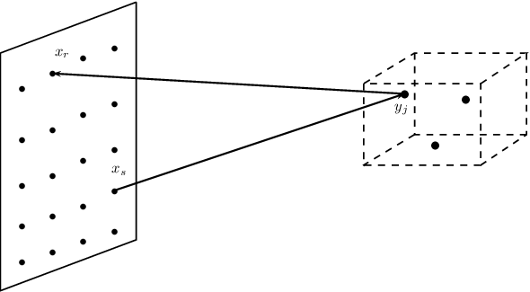
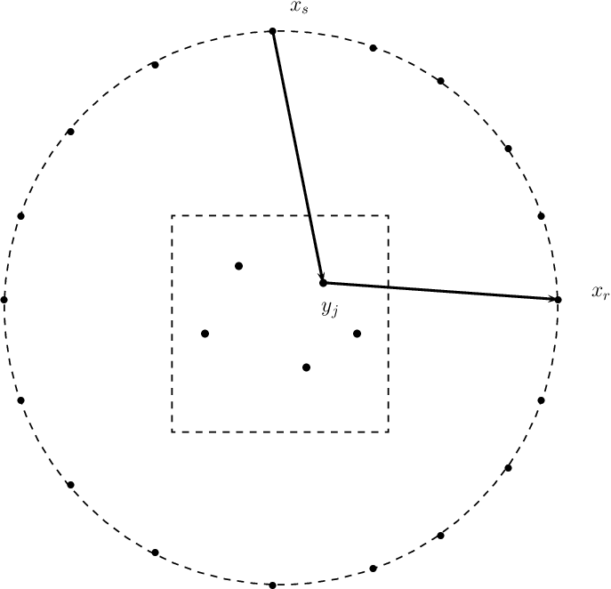
We have already discussed that the performance of sparsity promoting algorithms strongly depends on the mutual coherence of the sensing matrix, which is related to the array imaging configuration. In this section, we give some analytical results for the mutual coherence of two types of arrays that are often used in array imaging: planar arrays and spherical arrays. The schemata of these two types are illustrated in Figure 1. We show that under similar configurations of the IW (distance to the array and the resolution), spherical arrays give smaller upper bounds of the inner products of the normalized Green’s function vectors than planar arrays in condition (21). We give the proofs in Appendix C.
Refer to caption Refer to caption
Figure 1: Schemata of spherical (left) and planar (right) arrays

The first result is on the estimate of the inner product when a spherical array surrounding the IW is used. It is a well-known classical result. We state it here to be self-contained.

Proposition 5.1.

Assume that the IW is fully surrounded by a spherical array of radius LL. Given any two points 𝐲k\mbox{\boldmath{$y$}}_{k} and 𝐲k′\mbox{\boldmath{$y$}}_{k^{\prime}} in the IW such that λ≪|𝐲k−𝐲k′|≪L\lambda\ll|\mbox{\boldmath{$y$}}_{k}-\mbox{\boldmath{$y$}}_{k^{\prime}}|\ll L, we have

𝒈^0∗​(𝒚k)​𝒈^0​(𝒚k′)‖𝒈^0​(𝒚k)‖ℓ2​‖𝒈^0​(𝒚k′)‖ℓ2≈sinc⁡(κ​|𝒚k−𝒚k′|)∼1κ​|𝒚k−𝒚k′|.\frac{\mbox{\boldmath{$\widehat{g}$}}_{0}^{\ast}(\mbox{\boldmath{$y$}}_{k})\mbox{\boldmath{$\widehat{g}$}}_{0}(\mbox{\boldmath{$y$}}_{k^{\prime}})}{\|\mbox{\boldmath{$\widehat{g}$}}_{0}(\mbox{\boldmath{$y$}}_{k})\|_{\ell_{2}}\|\mbox{\boldmath{$\widehat{g}$}}_{0}(\mbox{\boldmath{$y$}}_{k^{\prime}})\|_{\ell_{2}}}\approx\operatorname{sinc}(\kappa|\mbox{\boldmath{$y$}}_{k}-\mbox{\boldmath{$y$}}_{k^{\prime}}|)\sim\frac{1}{\kappa|\mbox{\boldmath{$y$}}_{k}-\mbox{\boldmath{$y$}}_{k^{\prime}}|}\,. (39)

Hence, the mutual coherence condition of the sensing matrix for spherical arrays is improved at the rate of the pixel size relative to the wavelength.

The second result is on the estimate when a planar array is used.

Proposition 5.2.

Assume a planar array of finite size and let 𝐲k\mbox{\boldmath{$y$}}_{k} and 𝐲k′\mbox{\boldmath{$y$}}_{k^{\prime}} be two points within the IW such that λ≪|𝐲k−𝐲k′|≪L\lambda\ll|\mbox{\boldmath{$y$}}_{k}-\mbox{\boldmath{$y$}}_{k^{\prime}}|\ll L. Then, we have

𝒈^0∗​(𝒚k)​𝒈^0​(𝒚k′)‖𝒈^0​(𝒚k)‖ℓ2​‖𝒈^0​(𝒚k′)‖ℓ2∼1κ​|𝒚k−𝒚k′|.\frac{\mbox{\boldmath{$\widehat{g}$}}_{0}^{\ast}(\mbox{\boldmath{$y$}}_{k})\mbox{\boldmath{$\widehat{g}$}}_{0}(\mbox{\boldmath{$y$}}_{k^{\prime}})}{\|\mbox{\boldmath{$\widehat{g}$}}_{0}(\mbox{\boldmath{$y$}}_{k})\|_{\ell_{2}}\|\mbox{\boldmath{$\widehat{g}$}}_{0}(\mbox{\boldmath{$y$}}_{k^{\prime}})\|_{\ell_{2}}}\sim\frac{1}{\sqrt{\kappa|\mbox{\boldmath{$y$}}_{k}-\mbox{\boldmath{$y$}}_{k^{\prime}}|}}. (40)

Hence, the mutual coherence condition of the sensing matrix for planar arrays is improved at the rate of square root of the pixel size relative to the wavelength.

Based on these results, the upper bound of (24) is smaller for spherical arrays than for planar arrays. The pixel size of the IW with which good images are obtained is smaller for spherical arrays than for planar arrays. According to the analyses in §3 and §4, array imaging with spherical arrays can then locate more scatterers with higher resolution and is more robust with respect to the additive noise than array imaging with planar arrays, provided all other conditions are identical. This observation is supported by the numerical experiments.

6 Numerical simulation

In this section we present numerical simulations in two dimensions. The linear array consists of 100100 transducers that are one wavelength λ\lambda apart. Five scatterers are placed within an IW of size 41​λ×41​λ41\lambda\times 41\lambda which is at a distance L=100​λL=100\lambda from the linear array. The amplitudes of the reflectivities of the scatterers, |αj||\alpha_{j}|, are 2.962.96, 2.762.76, 2.052.05, 1.541.54 and 1.351.35 (see Fig. 2). Their phases are set randomly in each realization. We note that, given an illumination vector 𝒇^\widehat{f} and a scatterer configuration 𝝆0\mbox{\boldmath{$\rho$}}_{0} with fixed amplitudes, the exact amount of multiple scattering depends on the realization of the phases in 𝝆0\mbox{\boldmath{$\rho$}}_{0}. For the amplitudes of the reflectivities chosen here, the amount of multiple scattering, defined by

‖𝑷^−𝑷^s​s‖F‖𝑷^s​s‖F×100,\frac{\|\mbox{\boldmath{$\widehat{P}$}}-\mbox{\boldmath{$\widehat{P}$}}_{ss}\|_{F}}{\|\mbox{\boldmath{$\widehat{P}$}}_{ss}\|_{F}}\times 100\,, (41)

typically ranges between 50%50\% and 100%100\% in the simulations shown below. In (41), 𝑷^s​s\mbox{\boldmath{$\widehat{P}$}}_{ss} is the response matrix without multiple scatterering, computed by replacing 𝒢F​LT​(𝝆0)\mbox{\boldmath{${\cal G}$}}_{FL}^{T}(\mbox{\boldmath$\rho$}_{0}) by 𝒢T\mbox{\boldmath{${\cal G}$}}^{T} in (15), i.e., 𝑷^s​s=𝒢​diag⁡(𝝆)​𝒢T\mbox{\boldmath{$\widehat{P}$}}_{ss}=\mbox{\boldmath{${\cal G}$}}\operatorname{diag}(\mbox{\boldmath$\rho$})\mbox{\boldmath{${\cal G}$}}^{T}.

The five scatterers are within an IW that is discretized using a uniform lattice with points separated by one wavelength λ\lambda. This results in a 41×4141\times 41 uniform mesh. Hence, we have 16811681 unknowns and 100100 measurements. In all the images shown below, we normalize the spatial units by the wavelength λ\lambda. For this configuration of the IW, the mutual coherence (24) of the sensing matrix 𝒢{\cal G} has a numerical value equal to 0.980.98. This, together with M=5M=5 scatterers, clearly violates the sufficient condition for stable reconstruction required by formulations using either single illumination or multiple illuminations. However, this condition is quite conservative and we will show that the images are still good when the noise level is low in the data. Finally, we note that the obtained images depend on the realization of the random phases of the scatterers. In all the images shown below, we do not display the ones with the best quality we have seen in our numerical study.

Refer to caption
Figure 2: Original configuration of the scatterers in a 41×4141\times 41 image window with grid points separated by 11. The amplitudes of the reflectivities of the scatterers, |αj||\alpha_{j}|, are 2.962.96, 2.762.76, 2.052.05, 1.541.54 and 1.351.35.

Figure 3 shows the results of ℓ1\ell_{1} norm minimization with 0%0\% (left), 10%10\% (middle) and 20%20\% noise (right) when a single illumination coming from the center of the array is used. The exact locations of the scatterers in these images are indicated with small white dots. When there is no noise in the data, ℓ1\ell_{1} norm minimization recovers the positions and reflectivities of the scatterers accurately. However, when 10%10\% and 20%20\% of noise is added to the data, the method fails to recover some of the scatterers and the images show some ghosts. Note that some scatterers are missing in the middle and right images of Figure 3.

Refer to caption Refer to caption Refer to caption
Figure 3: Images reconstructed by solving (19) and (20) when single illumination is used. From left to right, there is 0%0\%, 10%10\%, and 20%20\% noise in the data.

In order to stabilize the images, we study the improvement of the results when data collected with multiple illuminations are used. We consider first the case where the illuminations are randomly selected. By random illuminations we mean several illuminations coming, each one, from only one of the transducers on the array at a time, i.e., f^p=1\widehat{f}_{p}=1 and f^q=0\widehat{f}_{q}=0 for q≠pq\neq p, with pp chosen randomly at a time. Figure 4 shows the results of the MMV algorithm when 55 (top row) and 1515 (bottom row) random illuminations are used. Additive noise at level 10%10\% (left column), 20%20\% (middle column) and 50%50\% (right column) is added to the data in these numerical experiments. As expected, the images obtained with multiple illuminations are more stable with respect to additive noise. In fact, only a small number of illuminations are needed to improve the imaging performance significantly. However, it is not always true in general that more random illuminations always lead to better images. For instance, the image obtained with 20%20\% noise and 1515 random illuminations (middle image of the bottom row) is worse than that obtained with 20%20\% noise and 55 random illuminations (middle image of the top row). This is so because the illuminations are chosen randomly and “good” illuminations that lead to enough data diversity cannot be guaranteed.

Refer to caption Refer to caption Refer to caption
Figure 4: Images reconstructed by solving (32) when 55 (top row) and 1515 (bottom row) random illuminations are used. From left to right, there is 10%10\%, 20%20\%, and 50%50\% noise in the data.

Figure 4 indicates the importance of selecting “good” illuminations in the MMV formulation and suggests the use of optimal illuminations, especially when the signal-to-noise ratio (SNR) is low. Using optimal illuminations means taking 𝒇^j=𝑽^⋅j\mbox{\boldmath{$\widehat{f}$}}^{j}=\mbox{\boldmath{$\widehat{V}$}}_{\cdot j}, j=1,…,Mj=1,\ldots,M, as illuminations. These vectors can be obtained through the SVD of the array response matrix 𝑷^\widehat{P} or by iterative time reversal. Note that, by choosing the illuminations optimally, we (i) maximize the data diversity, which also means low unnecessary redundancy of the multiple illuminations; and (ii) we reduce the noisy terms contained in the data matrix 𝐁\mathbf{B}. On the other hand, we point out that, in principle, this approach would require the prior knowledge of the number of scatterers MM if the noise level is high and is difficult to determine the singular values that correspond to the signal space. Hence, it is important to investigate the robustness of this approach with respect to the number of optimal illuminations used in the scheme. In Figure 5 we display the results when an increasing number of optimal illuminations are used. From left to right, and from top to bottom, we use 11, 22, 33, 44, 55, and 1212 illuminations associated to the corresponding singular vectors 𝑽^⋅j\mbox{\boldmath{$\widehat{V}$}}_{\cdot j}, with j=1,2,3,4,5,12j=1,2,3,4,5,12. We observe that this approach is very robust with respect to the number of optimal illuminations used. It is remarkable that only a few of them (22 or 33) are enough to achieve a significant improvement. Furthermore, using many more singular vectors as illuminations does not deteriorate too much the images (see the right image in the bottom row, where 1212 illuminations are use). Finally, we point out that when multiple scattering is negligible all the significant singular vectors are necessary as shown in [5]. In that case, each optimal illumination aims at one scatterer at a time, provided that the array is large enough.

Refer to caption Refer to caption Refer to caption
Figure 5: Images reconstructed by solving (32) when optimal illuminations are used. There is 50%50\% noise in the data. From left to right and top to bottom, images are reconstructed by using 11, 22, 33, 44, 55, and 1212 top singular vectors.
Refer to caption Refer to caption Refer to caption
Figure 6: Images reconstructed by MUSIC. There is 50%50\% noise in the data. From left to right and top to bottom, images are reconstructed by using 11, 22, 33, 44, 55, and 1212 top singular vectors.

We compare the images obtained with the MMV formulation and optimal illuminations, with those obtained with MUSIC. These two methods assume knowledge of the significant singular vectors of the response matrix 𝑷^\widehat{P} to form the images. Thus, the comparison between these two method is carried out with about the same amount of data. In Figure 6 we show the images obtained with MUSIC when an increasing number of significant singular vectors of the response matrix 𝑷^\widehat{P} are used. As expected, we observe that MUSIC needs to use a number of singular vectors equal or greater to the number of scatterers. This is so, because MUSIC is a subspace based imaging technique that needs all the significant singular vectors to span the signal spaced. In other words, the complementary space representing the noise has to be correctly constructed such that no true signals should fall into. We also observe that the images formed with MUSIC do not change much when the number of singular vectors used exceeds the number of scatterers. These differences between MMV and MUSIC when both use the essential data of the response matrix 𝑷^\widehat{P} is also observed in [17] in the context of DOA for the localization of sources with sensor arrays.

7 Conclusion

We give a novel approach to imaging localized scatterers with non-negligible multiple scattering between them. Our approach is non-iterative and solves the problem in two steps using sparsity promoting optimization. The uniqueness and stability of the formulations using both single and multiple illuminations are analyzed. We also propose to apply optimal illuminations to improve the robustness of the imaging methods and the resolution of the images. We show that the conditions under which the proposed methods work well are related to the configuration of the imaging problems: spherical arrays are in general more favorable than planar arrays. We illustrated the theoretical results with various numerical examples.

Appendix

Appendix A Proof of Theorem 4.1

We prove Theorem 4.1 by proving a more general result given below.

Theorem A.1.

For a given array configuration, assume that the resolution of the IW satisfies (21). If the number of scatterers MM is such that M​ϵ<1/2M\epsilon<1/2, then 𝐗0=[𝛄01​…​𝛄0ν]\mbox{\boldmath{${X}$}}_{0}=[\mbox{\boldmath$\gamma$}_{0}^{1}\,\ldots\,\mbox{\boldmath$\gamma$}_{0}^{\nu}] is the unique solution to

min⁡Jp,1​(𝑿)s.t.𝒢𝐗=𝐁\min J_{p,1}(\mbox{\boldmath{${X}$}})\quad\text{s.t.}\quad\mbox{\boldmath{${\cal G}$}}\mbox{\boldmath{${X}$}}=\mathbf{B}

for any 1<p<∞1<p<\infty.

Clearly, Theorem 4.1 is a special case of Theorem A.1. The proof of Theorem A.1 is an application of the following result which is a generalization of Theorem 3.13.1 in [11].

Proposition A.2.

Let Λ\Lambda be the set of row support of 𝐗0\mbox{\boldmath{${X}$}}_{0}, i.e. Λ=rowsupp⁡(𝐗0)\Lambda=\operatorname{rowsupp}(\mbox{\boldmath{${X}$}}_{0}). For any 1<p<∞1<p<\infty and a matrix 𝐐\mathbf{Q}, define

sign⁡(Qi​j)={|Qi​j|p−1​sign⁡(Qi​j)∥|Qi⋅|p−1∥ℓq,‖Qi,⋅‖ℓq≠00,‖Qi,⋅‖ℓq=0,\operatorname{sign}(Q_{ij})=\begin{cases}\frac{|Q_{ij}|^{p-1}\operatorname{sign}(Q_{ij})}{\||Q_{i\cdot}|^{p-1}\|_{\ell_{q}}},&\|Q_{i,\cdot}\|_{\ell_{q}}\neq 0\\ 0,&\|Q_{i,\cdot}\|_{\ell_{q}}=0,\end{cases}

where sign⁡(x)=0,±1\operatorname{sign}(x)=0,\pm 1 when x∈ℝx\in\mathbb{R} and sign⁡(x)=exp⁡(i​angle⁡(x))\operatorname{sign}(x)=\exp(\mathrm{i}\operatorname{angle}(x)) when x∈ℂx\in\mathbb{C}. Also assume 𝒢Λ\mbox{\boldmath{${\cal G}$}}_{\Lambda}, submatrix of 𝒢{\cal G} consisting of columns with indices in Λ\Lambda, is non-singular. Then a sufficient condition under which 𝐗0\mbox{\boldmath{${X}$}}_{0} is the unique solution to

min𝑿⁡Jp,1​(𝑿)s.t.𝒢𝐗=𝐁\min_{\mbox{\boldmath{${X}$}}}J_{p,1}(\mbox{\boldmath{${X}$}})\quad\text{s.t.}\quad\mbox{\boldmath{${\cal G}$}}\mbox{\boldmath{${X}$}}=\mathbf{B}

is that there exists a matrix 𝐇∈ℂN×ν\mathbf{H}\in\mathbb{C}^{N\times\nu} satisfying

𝒢Λ∗​𝐇=sign⁡(𝑿0​Λ)\mbox{\boldmath{${\cal G}$}}_{\Lambda}^{\ast}\mathbf{H}=\operatorname{sign}(\mbox{\boldmath{${X}$}}_{0\Lambda}) (42)

and

‖𝐇∗​𝒈^0​(𝒚j)‖ℓq<1,\|\mathbf{H}^{\ast}\mbox{\boldmath{$\widehat{g}$}}_{0}(\mbox{\boldmath{$y$}}_{j})\|_{\ell_{q}}<1, (43)

where 1/p+1/q=11/p+1/q=1 and 𝐗0​Λ\mbox{\boldmath{${X}$}}_{0\Lambda} is the submatrix consisting of the rows of 𝐗0\mbox{\boldmath{${X}$}}_{0} in Λ\Lambda.

To prove Proposition A.2, we need the following lemma.

Lemma A.3.

For any two matrices A∈ℂm×lA\in\mathbb{C}^{m\times l} and B∈ℂl×nB\in\mathbb{C}^{l\times n}, we have

|trace⁡(A​B)|≤maxk=1,…,l⁡‖B⋅k‖ℓq​Jp,1​(A).\big|\operatorname{trace}(AB)\big|\leq\max_{k=1,\ldots,l}\|B_{\cdot k}\|_{\ell_{q}}\,J_{p,1}(A).

The strict inequality holds when there exists kk such that ‖B⋅k‖ℓq<maxk=1,…,l⁡‖B⋅k‖ℓq\|B_{\cdot k}\|_{\ell_{q}}<\max_{k=1,\ldots,l}\|B_{\cdot k}\|_{\ell_{q}} and ∥Ak⋅∥ℓp≠0\|A_{k\cdot}\|_{\ell_{p}}\neq 0.

Proof.

By definition of trace, we have

|trace(AB)|≤∑k=1l|Ak⋅B⋅k|≤∑k=1l∥Ak⋅∥ℓp∥B⋅k∥ℓq≤maxk=1,…,l∥B⋅k∥ℓqJp,1(A)|\operatorname{trace}(AB)|\leq\sum_{k=1}^{l}|A_{k\cdot}B_{\cdot k}|\leq\sum_{k=1}^{l}\|A_{k\cdot}\|_{\ell_{p}}\|B_{\cdot k}\|_{\ell_{q}}\leq\max_{k=1,\ldots,l}\|B_{\cdot k}\|_{\ell_{q}}\,J_{p,1}(A)

where we use the Hölder’s inequality in the second to last inequality. The strict inequality apparently holds when the condition is satisfied. ∎

Proof of Proposition A.2.

We will show the uniqueness by contradiction. Assume there exists another solution 𝑿^\widehat{\mbox{\boldmath{${X}$}}} the support of which is Λ^\widehat{\Lambda} such that Λ^\Λ≠∅\widehat{\Lambda}\backslash\Lambda\neq\emptyset. First of all, notice that (42), (43) imply that for any column of 𝒢{\cal G}, ‖𝐇∗​𝒈^0​(𝒚j)‖ℓq≤1\|\mathbf{H}^{\ast}\mbox{\boldmath{$\widehat{g}$}}_{0}(\mbox{\boldmath{$y$}}_{j})\|_{\ell_{q}}\leq 1. We have

Jp,1​(𝑿0)=Jp,1​(𝑿0​Λ)=trace⁡(sign⁡(𝑿0​Λ)​𝑿0​Λ∗)=trace⁡(𝒢Λ∗​𝐇​𝑿0​Λ∗).J_{p,1}(\mbox{\boldmath{${X}$}}_{0})=J_{p,1}(\mbox{\boldmath{${X}$}}_{0\Lambda})=\operatorname{trace}(\operatorname{sign}(\mbox{\boldmath{${X}$}}_{0\Lambda})\mbox{\boldmath{${X}$}}_{0\Lambda}^{\ast})=\operatorname{trace}(\mbox{\boldmath{${\cal G}$}}_{\Lambda}^{\ast}\mathbf{H}\mbox{\boldmath{${X}$}}_{0\Lambda}^{\ast}).

Since the trace\operatorname{trace} function is invariant with respect to matrix rotation and transpose operation,

Jp,1​(𝑿0)=trace⁡(𝑿0​Λ​𝐇∗​𝒢Λ)=trace⁡(𝐇∗​𝒢Λ​𝑿0​Λ)=trace⁡(𝐇∗​𝒢​𝑿^).J_{p,1}(\mbox{\boldmath{${X}$}}_{0})=\operatorname{trace}(\mbox{\boldmath{${X}$}}_{0\Lambda}\mathbf{H}^{\ast}\mbox{\boldmath{${\cal G}$}}_{\Lambda})=\operatorname{trace}(\mathbf{H}^{\ast}\mbox{\boldmath{${\cal G}$}}_{\Lambda}\mbox{\boldmath{${X}$}}_{0\Lambda})=\operatorname{trace}(\mathbf{H}^{\ast}\mbox{\boldmath{${\cal G}$}}\widehat{\mbox{\boldmath{${X}$}}}).

Applying Lemma A.3, we have

Jp,1​(𝑿0)≤maxj∈Λ^⁡‖𝐇∗​𝒈^0​(𝒚j)‖ℓq​Jp,1​(𝑿^)≤Jp,1​(𝑿^).J_{p,1}(\mbox{\boldmath{${X}$}}_{0})\leq\max_{j\in\widehat{\Lambda}}\|\mathbf{H}^{\ast}\mbox{\boldmath{$\widehat{g}$}}_{0}(\mbox{\boldmath{$y$}}_{j})\|_{\ell_{q}}\,J_{p,1}(\widehat{\mbox{\boldmath{${X}$}}})\leq J_{p,1}(\widehat{\mbox{\boldmath{${X}$}}}).

Because Λ^\Λ≠∅\widehat{\Lambda}\backslash\Lambda\neq\emptyset, there must exist j0∈Λ^j_{0}\in\widehat{\Lambda} such that ‖𝐇∗​𝒈^0​(𝒚j0)‖ℓq≠maxj∈Λ^⁡‖𝐇∗​𝒈^0​(𝒚j)‖ℓq\|\mathbf{H}^{\ast}\mbox{\boldmath{$\widehat{g}$}}_{0}(\mbox{\boldmath{$y$}}_{j_{0}})\|_{\ell_{q}}\neq\max_{j\in\widehat{\Lambda}}\|\mathbf{H}^{\ast}\mbox{\boldmath{$\widehat{g}$}}_{0}(\mbox{\boldmath{$y$}}_{j})\|_{\ell_{q}}. On the other hand, since the support of 𝑿^\widehat{\mbox{\boldmath{${X}$}}} is Λ^\widehat{\Lambda}, we have ∥X^j⋅∥ℓq≠0\|\widehat{X}_{j\cdot}\|_{\ell_{q}}\neq 0 for any j∈Λ^j\in\widehat{\Lambda}. According to Lemma A.3, Jp,1​(𝑿0)<Jp,1​(𝑿^)J_{p,1}(\mbox{\boldmath{${X}$}}_{0})<J_{p,1}(\widehat{\mbox{\boldmath{${X}$}}}) which contradicts that 𝑿^\widehat{\mbox{\boldmath{${X}$}}} is also a solution. Therefore, the solution must be unique. ∎

Now we will show that the multiplier 𝐇\mathbf{H} satisfying (42) and (43) exists under the condition of Theorem A.1.

Proof of Theorem A.1.

Let Λ={nj,1≤j≤M}\Lambda=\{n_{j},1\leq j\leq M\} be the set of indices corresponding to the scatterers. Based on the resolution condition, we have that the inner product of the column vectors of the matrix 𝒢{\cal G} satisfies 𝒈^0∗​(𝒚i)​𝒈^0​(𝒚j)=δi​j+(1−δi​j)​ϵi​j\mbox{\boldmath{$\widehat{g}$}}_{0}^{\ast}(\mbox{\boldmath{$y$}}_{i})\mbox{\boldmath{$\widehat{g}$}}_{0}(\mbox{\boldmath{$y$}}_{j})=\delta_{ij}+(1-\delta_{ij})\epsilon_{ij} with |ϵi​j|<ϵ|\epsilon_{ij}|<\epsilon, for any 1≤i,j≤M1\leq i,j\leq M. Therefore, the submatrix 𝒢Λ\mbox{\boldmath{${\cal G}$}}_{\Lambda}, composed of the columns n1,…,nMn_{1},\ldots,n_{M} of matrix 𝒢{\cal G}, is full column rank and satisfies that 𝒢Λ∗​𝒢Λ\mbox{\boldmath{${\cal G}$}}_{\Lambda}^{\ast}\mbox{\boldmath{${\cal G}$}}_{\Lambda} is full rank and diagonally dominant.

According to Proposition A.2, we need to find a matrix 𝐇\mathbf{H} satisfying (42) and (43). Let 𝐇=𝒢Λ​(𝒢Λ∗​𝒢Λ)−1​sign⁡(𝑿0​Λ)\mathbf{H}=\mbox{\boldmath{${\cal G}$}}_{\Lambda}(\mbox{\boldmath{${\cal G}$}}_{\Lambda}^{\ast}\mbox{\boldmath{${\cal G}$}}_{\Lambda})^{-1}\operatorname{sign}(\mbox{\boldmath{${X}$}}_{0\Lambda}). Then, the first condition is automatically satisfied because 𝒢Λ∗​𝐇=sign⁡(𝑿0​Λ)\mbox{\boldmath{${\cal G}$}}_{\Lambda}^{\ast}\mathbf{H}=\operatorname{sign}(\mbox{\boldmath{${X}$}}_{0\Lambda}). For the second condition, choosing any column jj of 𝒢{\cal G} not in the submatrix 𝒢Λ\mbox{\boldmath{${\cal G}$}}_{\Lambda}, we have

‖𝒈^0∗​(𝒚j)​𝒢Λ​(𝒢Λ∗​𝒢Λ)−1​sign⁡(𝑿0​Λ)‖ℓq\displaystyle\|\mbox{\boldmath{$\widehat{g}$}}_{0}^{\ast}(\mbox{\boldmath{$y$}}_{j})\mbox{\boldmath{${\cal G}$}}_{\Lambda}(\mbox{\boldmath{${\cal G}$}}_{\Lambda}^{\ast}\mbox{\boldmath{${\cal G}$}}_{\Lambda})^{-1}\operatorname{sign}(\mbox{\boldmath{${X}$}}_{0\Lambda})\|_{\ell_{q}} ≤\displaystyle\leq ‖sign⁡(𝑿0​Λ)‖p→∞​‖(𝒢Λ∗​𝒢Λ)−1‖ℓ1​‖𝒢Λ∗​𝒈^0​(𝒚j)‖ℓ1\displaystyle\|\operatorname{sign}(\mbox{\boldmath{${X}$}}_{0\Lambda})\|_{p\rightarrow\infty}\|(\mbox{\boldmath{${\cal G}$}}_{\Lambda}^{\ast}\mbox{\boldmath{${\cal G}$}}_{\Lambda})^{-1}\|_{\ell_{1}}\|\mbox{\boldmath{${\cal G}$}}_{\Lambda}^{\ast}\mbox{\boldmath{$\widehat{g}$}}_{0}(\mbox{\boldmath{$y$}}_{j})\|_{\ell_{1}}
≤\displaystyle\leq M​ϵ1−M​ϵ<1,\displaystyle\frac{M\epsilon}{1-M\epsilon}<1,

where by definition, we have ‖sign⁡(𝑿0​Λ)‖p→∞≤1\|\operatorname{sign}(\mbox{\boldmath{${X}$}}_{0\Lambda})\|_{p\rightarrow\infty}\leq 1 and the last inequality is due to the resolution condition M​ϵ<1/2M\epsilon<1/2. ∎

Appendix B Proof of Theorem 4.3

In [27], the author gives conditions for the MMV problem under which the convex relaxation formulation with functional J∞,1J_{\infty,1} is robust with respect to the additive noise. In the following, we derive similar conditions for convex relaxation using J2,1J_{2,1} instead of J∞,1J_{\infty,1}. This is done using the techniques developed in [24]. We first introduce some supporting results.

Let ff be a function from the complex matrix space ℳ{\cal M} to ℂ\mathbb{C}. The subdifferential of a function ff at 𝑿∈ℳ\mbox{\boldmath{${X}$}}\in{\cal M} is defined as

∂f(𝐗)={𝐆∈ℳ:f(𝐘)≥f(𝐗)+Re⟨𝐘−𝐗,𝐆⟩,∀𝐘∈ℳ}.\partial f(\mathbf{X})=\{\mathbf{G}\in{\cal M}:f(\mathbf{Y})\geq f(\mathbf{X})+\mbox{Re}\left\langle\mathbf{Y}-\mathbf{X},\mathbf{G}\right\rangle,\,\,\forall\,\,\mathbf{Y}\in{\cal M}\}\,.
Lemma B.1.

A matrix 𝐆\mathbf{G} lies in the subdifferential of J2,1​(𝐗)J_{2,1}(\mathbf{X}) at 𝐗∈ℂK×ν\mathbf{X}\in\mathbb{C}^{K\times\nu} if and only if its rows Gi⋅∈ℂνG_{i\cdot}\in\mathbb{C}^{\nu} satisfy

  • •

    Gi⋅=Xi⋅∥Xi⋅∥ℓ2G_{i\cdot}=\frac{X_{i\cdot}}{\|X_{i\cdot}\|_{\ell_{2}}} when Xi⋅≠0X_{i\cdot}\neq 0, and

  • •

    ∥Gi⋅∥ℓ2≤1\|G_{i\cdot}\|_{\ell_{2}}\leq 1 when Xi⋅=0X_{i\cdot}=0.

Moreover, 𝐆\mathbf{G} is called a subgradient of J2,1​(𝐗)J_{2,1}(\mathbf{X}) at 𝐗\mathbf{X}.

Then according to the definition of matrix norms, it is easy to see the subgradient of J2,1J_{2,1} satisfies the following.

Corollary B.2.

Any subgradient 𝐆\mathbf{G} of J2,1J_{2,1} satisfies ‖𝐆‖2→∞=‖𝐆∗‖1,2≤1\|\mathbf{G}\|_{2\rightarrow\infty}=\|\mathbf{G}^{\ast}\|_{1,2}\leq 1.

We now give a result related to operator norms of matrices which will be used later.

Lemma B.3.

For any given matrix 𝐀\mathbf{A}, we have ‖𝐀‖(2,∞)→F≤‖𝐀‖∞→2\|\mathbf{A}\|_{(2,\infty)\rightarrow F}\leq\|\mathbf{A}\|_{\infty\rightarrow 2}.

Proof.

Let 𝐀\mathbf{A} be an m×nm\times n matrix. By definition, we have

‖𝐀‖(2,∞)→F=max𝐂∈ℝn×d⁡‖𝐀𝐂‖F‖𝐂‖2→∞.\|\mathbf{A}\|_{(2,\infty)\rightarrow F}=\max_{\mathbf{C}\in\mathbb{R}^{n\times d}}\frac{\|\mathbf{AC}\|_{F}}{\|\mathbf{C}\|_{2\rightarrow\infty}}.

Since we have

(‖𝐀𝐂‖F‖𝐂‖2→∞)2\displaystyle\left(\frac{\|\mathbf{AC}\|_{F}}{\|\mathbf{C}\|_{2\rightarrow\infty}}\right)^{2} =\displaystyle= ∑i=1m∑j=1d|∑k=1nAi​k​Ck​j|2max1≤i≤n∥Ci⋅∥ℓ22\displaystyle\frac{\sum_{i=1}^{m}\sum_{j=1}^{d}\bigg|\sum_{k=1}^{n}A_{ik}C_{kj}\bigg|^{2}}{\max_{1\leq i\leq n}\|C_{i\cdot}\|_{\ell_{2}}^{2}}
≤\displaystyle\leq ∑i=1m|∑k=1nAi​k∥Ck⋅∥ℓ2|2max1≤i≤n∥Ci⋅∥ℓ22\displaystyle\frac{\sum_{i=1}^{m}\bigg|\sum_{k=1}^{n}A_{ik}\|C_{k\cdot}\|_{\ell_{2}}\bigg|^{2}}{\max_{1\leq i\leq n}\|C_{i\cdot}\|_{\ell_{2}}^{2}}
≤\displaystyle\leq max𝒄∈ℝn⁡(‖𝐀​𝒄‖ℓ2‖𝒄‖∞)2\displaystyle\max_{\mbox{\boldmath{$c$}}\in\mathbb{R}^{n}}\left(\frac{\|\mathbf{A}\mbox{\boldmath{$c$}}\|_{\ell_{2}}}{\|\mbox{\boldmath{$c$}}\|_{\infty}}\right)^{2}
≤\displaystyle\leq ‖𝐀‖∞→22,\displaystyle\|\mathbf{A}\|^{2}_{\infty\rightarrow 2},

it is clearly that ‖𝐀‖(2→∞)→F≤‖𝐀‖∞→2\|\mathbf{A}\|_{(2\rightarrow\infty)\rightarrow F}\leq\|\mathbf{A}\|_{\infty\rightarrow 2}. In the derivation above, the first inequality is true because for each row index ii, we have

∑j=1d|∑k=1nAi​k​Ck​j|2\displaystyle\sum_{j=1}^{d}\bigg|\sum_{k=1}^{n}A_{ik}C_{kj}\bigg|^{2} =\displaystyle= ∑j=1d∑k,k′=1nAi​k​Ck​j​A¯i​k′​C¯k′​j\displaystyle\sum_{j=1}^{d}\sum_{k,k^{\prime}=1}^{n}A_{ik}C_{kj}\bar{A}_{ik^{\prime}}\bar{C}_{k^{\prime}j}
=\displaystyle= ∑k,k′=1nAi​k​A¯i​k′​∑j=1dCk​j​C¯k′​j\displaystyle\sum_{k,k^{\prime}=1}^{n}A_{ik}\bar{A}_{ik^{\prime}}\sum_{j=1}^{d}C_{kj}\bar{C}_{k^{\prime}j}
=\displaystyle= ∑k,k′=1nAi​kA¯i​k′⟨Ck⋅,Ck′⋅⟩\displaystyle\sum_{k,k^{\prime}=1}^{n}A_{ik}\bar{A}_{ik^{\prime}}\langle C_{k\cdot},C_{k^{\prime}\cdot}\rangle
≤\displaystyle\leq ∑k,k′=1nAi​kA¯i​k′∥Ck⋅∥ℓ2∥Ck′⋅∥ℓ2\displaystyle\sum_{k,k^{\prime}=1}^{n}A_{ik}\bar{A}_{ik^{\prime}}\|C_{k\cdot}\|_{\ell_{2}}\|C_{k^{\prime}\cdot}\|_{\ell_{2}}
=\displaystyle= |∑k=1nAi​k∥Ck⋅∥ℓ2|2.\displaystyle\left|\sum_{k=1}^{n}A_{ik}\|C_{k\cdot}\|_{\ell_{2}}\right|^{2}.

∎

To make the following discussion easier, we assume that the sensing matrix 𝒢{\cal G} has normalized columns and we introduce some additional notations used in this appendix only. Let Λ\Lambda be indexes of a subset of linearly independent columns of 𝒢{\cal G}, i.e. Λ⊂{1,2,…,K}\Lambda\subset\{1,2,\ldots,K\} such that the Green’s function vectors 𝒈^0​(𝒚j)\mbox{\boldmath{$\widehat{g}$}}_{0}(\mbox{\boldmath{$y$}}_{j}), with j∈Λj\in\Lambda, are linearly independent. We denote by 𝒢Λ∈ℂN×|Λ|\mbox{\boldmath{${\cal G}$}}_{\Lambda}\in\mathbb{C}^{N\times|\Lambda|} the submatrix of 𝒢{\cal G} composed of columns with indices in Λ\Lambda, by 𝐁Λ∈ℂN×ν\mathbf{B}_{\Lambda}\in\mathbb{C}^{N\times\nu} the best Frobenius norm approximation of the data matrix 𝐁\mathbf{B} over Λ\Lambda, and by 𝐗0​Λ∈ℂ|Λ|×ν\mathbf{X}_{0\Lambda}\in\mathbb{C}^{|\Lambda|\times\nu} the corresponding coefficent matrix synthesizing 𝐁Λ\mathbf{B}_{\Lambda}, i.e. such that 𝐁Λ=𝒢Λ​𝐗0​Λ\mathbf{B}_{\Lambda}=\mbox{\boldmath{${\cal G}$}}_{\Lambda}\mathbf{X}_{0\Lambda}. Note that 𝐗0​Λ=𝒢Λ†​𝐁Λ\mathbf{X}_{0\Lambda}=\mbox{\boldmath{${\cal G}$}}_{\Lambda}^{\dagger}\mathbf{B}_{\Lambda}, with 𝒢Λ†=(𝒢Λ∗​𝒢Λ)−1​𝒢Λ∗\mbox{\boldmath{${\cal G}$}}_{\Lambda}^{\dagger}=(\mbox{\boldmath{${\cal G}$}}_{\Lambda}^{\ast}\mbox{\boldmath{${\cal G}$}}_{\Lambda})^{-1}\mbox{\boldmath{${\cal G}$}}_{\Lambda}^{\ast}.

Next, we give several results related to the minimizers of the Lagrange function (37). The proofs are analogue to those in [27] and will be skipped. Interested readers can refer to [27] or [24] for single measurement case. The first lemma is on the condition of the minimizer of (37).

Lemma B.4.

Suppose that the matrix 𝐗⋆\mathbf{X}_{\star} is the minimizer of (37) over all matrices with row-support Λ\Lambda. A necessary and sufficient condition for 𝐗⋆\mathbf{X}_{\star} to be such minimizer is that

𝐗0​Λ−𝐗⋆=λ​(𝒢Λ∗​𝒢Λ)−1​𝐆,\mathbf{X}_{0\Lambda}-\mathbf{X}_{\star}=\lambda(\mbox{\boldmath{${\cal G}$}}_{\Lambda}^{\ast}\mbox{\boldmath{${\cal G}$}}_{\Lambda})^{-1}\mathbf{G}, (44)

where 𝐆∈∂J2,1​(𝐗⋆)\mathbf{G}\in\partial J_{2,1}(\mathbf{X}_{\star}). Moreover, the minimizer is unique.

Using Lemmas B.3 and  B.4, we have the following estimates on the bound of the minimizer of (37) over a specific support.

Lemma B.5.

Suppose that the matrix 𝐗⋆\mathbf{X}_{\star} is the unique minimizer of (37) over all matrices with support inside Λ\Lambda. Then, the following estimates hold:

‖𝐗0​Λ−𝐗⋆‖2→∞≤λ​‖(𝒢Λ∗​𝒢Λ)−1‖2→∞,\displaystyle\quad\|\mathbf{X}_{0\Lambda}-\mathbf{X}_{\star}\|_{2\rightarrow\infty}\leq\lambda\|(\mbox{\boldmath{${\cal G}$}}_{\Lambda}^{\ast}\mbox{\boldmath{${\cal G}$}}_{\Lambda})^{-1}\|_{2\rightarrow\infty}, (45)
‖𝒢Λ​(𝐗0​Λ−𝐗⋆)‖F≤λ​‖𝒢Λ†‖2→1.\displaystyle\quad\|\mbox{\boldmath{${\cal G}$}}_{\Lambda}(\mathbf{X}_{0\Lambda}-\mathbf{X}_{\star})\|_{F}\leq\lambda\|\mbox{\boldmath{${\cal G}$}}_{\Lambda}^{\dagger}\|_{2\rightarrow 1}\,. (46)

The above results are on the bounds of the error between 𝐗⋆\mathbf{X}_{\star} and the “true” solution 𝐗0​Λ\mathbf{X}_{0\Lambda} when the search is restricted to a given support Λ\Lambda. We now give a condition under which the solution 𝐗⋆\mathbf{X}_{\star} to (37) will be supported on Λ\Lambda. For this condition, we need to use the Exact Recovery Coefficient

E​R​C​(Λ)=1−maxj∉Λ⁡‖𝒢Λ†​𝒈^​(𝒚j)‖ℓ1,ERC(\Lambda)=1-\max_{j\not\in\Lambda}\|\mbox{\boldmath{${\cal G}$}}_{\Lambda}^{\dagger}\mbox{\boldmath{$\widehat{g}$}}(\mbox{\boldmath{$y$}}_{j})\|_{\ell_{1}}, (47)

introduced in [24], which measures the orthogonality between the column vectors used in 𝒢Λ\mbox{\boldmath{${\cal G}$}}_{\Lambda} and the remaining column vectors.

Lemma B.6.

Under the same condition as in Lemma B.5, if the following condition holds

‖𝒢∗​(𝐁−𝐁Λ)‖2→∞≤λ​E​R​C​(Λ),\|\mbox{\boldmath{${\cal G}$}}^{\ast}(\mathbf{B}-\mathbf{B}_{\Lambda})\|_{2\rightarrow\infty}\leq\lambda ERC(\Lambda), (48)

then the unique minimizer 𝐗⋆\mathbf{X}_{\star} of (37) is supported on Λ\Lambda.

Proof.

By definition, 𝐁Λ=𝒢Λ​𝐗0​Λ\mathbf{B}_{\Lambda}=\mbox{\boldmath{${\cal G}$}}_{\Lambda}\mathbf{X}_{0\Lambda}. Given any vector 𝒖∈ℂν\mbox{\boldmath{$u$}}\in\mathbb{C}^{\nu}, we have for any j∉Λj\not\in\Lambda,

|⟨𝒈^∗​(𝒚j)​(𝐁−𝒢Λ​𝐗0​Λ),𝒖⟩|=|⟨𝒈^∗​(𝒚j)​(𝐁−𝐁Λ),𝒖⟩|≤‖(𝐁−𝐁Λ)∗​𝒈^​(𝒚j)‖ℓ2​‖𝒖‖ℓ2|\langle\mbox{\boldmath{$\widehat{g}$}}^{\ast}(\mbox{\boldmath{$y$}}_{j})(\mathbf{B}-\mbox{\boldmath{${\cal G}$}}_{\Lambda}\mathbf{X}_{0\Lambda}),\mbox{\boldmath{$u$}}\rangle|=|\langle\mbox{\boldmath{$\widehat{g}$}}^{\ast}(\mbox{\boldmath{$y$}}_{j})(\mathbf{B}-\mathbf{B}_{\Lambda}),\mbox{\boldmath{$u$}}\rangle|\leq\|(\mathbf{B}-\mathbf{B}_{\Lambda})^{\ast}\mbox{\boldmath{$\widehat{g}$}}(\mbox{\boldmath{$y$}}_{j})\|_{\ell_{2}}\|\mbox{\boldmath{$u$}}\|_{\ell_{2}} (49)

and

|⟨𝒈^∗​(𝒚j)​𝒢Λ​(𝐗0​Λ−𝐗⋆),𝒖⟩|=|⟨𝒈^∗​(𝒚j)​𝒢Λ​(𝒢Λ∗​𝒢Λ)−1​𝐆,𝒖⟩|≤‖𝐆∗​𝒢Λ†​𝒈^​(𝒚j)‖ℓ2​‖𝒖‖ℓ2.|\langle\mbox{\boldmath{$\widehat{g}$}}^{\ast}(\mbox{\boldmath{$y$}}_{j})\mbox{\boldmath{${\cal G}$}}_{\Lambda}(\mathbf{X}_{0\Lambda}-\mathbf{X}_{\star}),\mbox{\boldmath{$u$}}\rangle|=|\langle\mbox{\boldmath{$\widehat{g}$}}^{\ast}(\mbox{\boldmath{$y$}}_{j})\mbox{\boldmath{${\cal G}$}}_{\Lambda}(\mbox{\boldmath{${\cal G}$}}_{\Lambda}^{\ast}\mbox{\boldmath{${\cal G}$}}_{\Lambda})^{-1}\mathbf{G},\mbox{\boldmath{$u$}}\rangle|\leq\|\mathbf{G}^{\ast}\mbox{\boldmath{${\cal G}$}}_{\Lambda}^{\dagger}\mbox{\boldmath{$\widehat{g}$}}(\mbox{\boldmath{$y$}}_{j})\|_{\ell_{2}}\|\mbox{\boldmath{$u$}}\|_{\ell_{2}}. (50)

Since 𝐗⋆\mathbf{X}_{\star} is the unique minimizer among all set of matrices with support included in Λ\Lambda, we only need to show that it is also the optimal solution among matrices with support larger than Λ\Lambda. Let 𝜻∈ℂK\mbox{\boldmath{$\zeta$}}\in\mathbb{C}^{K} be a standard unit vector with support on {1,…,K}\Λ\{1,\ldots,K\}\backslash\Lambda. Then, 𝐗⋆+𝜻𝒖∗\mathbf{X}_{\star}+\mbox{\boldmath{$\zeta$}}\mbox{\boldmath{$u$}}^{\ast} is a perturbation by adding a matrix with row support disjoint from that of 𝐗⋆\mathbf{X}_{\star}. If we compute the variation of (37) with respect to this perturbation, we obtain

L⁡(𝐗⋆+𝜻𝒖∗,λ)−L⁡(𝐗⋆,λ)\displaystyle L(\mathbf{X}_{\star}+\mbox{\boldmath{$\zeta$}}\mbox{\boldmath{$u$}}^{\ast},\lambda)-L(\mathbf{X}_{\star},\lambda) =\displaystyle= 12​(‖𝐁−𝒢​𝐗⋆−𝒈^​(𝒚j)​𝒖∗‖F2−‖𝐁−𝒢​𝐗⋆‖F2)+\displaystyle\frac{1}{2}(\|\mathbf{B}-\mbox{\boldmath{${\cal G}$}}\mathbf{X}_{\star}-\mbox{\boldmath{$\widehat{g}$}}(\mbox{\boldmath{$y$}}_{j})\mbox{\boldmath{$u$}}^{\ast}\|_{F}^{2}-\|\mathbf{B}-\mbox{\boldmath{${\cal G}$}}\mathbf{X}_{\star}\|_{F}^{2})+
λ⁡(J2,1​(𝐗⋆+𝜻𝒖∗)−J2,1​(𝐗⋆))\displaystyle\lambda(J_{2,1}(\mathbf{X}_{\star}+\mbox{\boldmath{$\zeta$}}\mbox{\boldmath{$u$}}^{\ast})-J_{2,1}(\mathbf{X}_{\star}))
=\displaystyle= 12​‖𝒈^​(𝒚j)​𝒖∗‖F2−Re⁡⟨𝐁−𝒢​𝐗⋆,𝒈^​(𝒚j)​𝒖∗⟩+λ​‖𝒖‖ℓ2\displaystyle\frac{1}{2}\|\mbox{\boldmath{$\widehat{g}$}}(\mbox{\boldmath{$y$}}_{j})\mbox{\boldmath{$u$}}^{\ast}\|_{F}^{2}-\operatorname{Re}\langle\mathbf{B}-\mbox{\boldmath{${\cal G}$}}\mathbf{X}_{\star},\mbox{\boldmath{$\widehat{g}$}}(\mbox{\boldmath{$y$}}_{j})\mbox{\boldmath{$u$}}^{\ast}\rangle+\lambda\|\mbox{\boldmath{$u$}}\|_{\ell_{2}}
=\displaystyle= 12​‖𝒈^​(𝒚j)​𝒖∗‖F2−Re⁡⟨𝒈^∗​(𝒚j)​(𝐁−𝒢Λ​𝐗0,Λ),𝒖∗⟩−\displaystyle\frac{1}{2}\|\mbox{\boldmath{$\widehat{g}$}}(\mbox{\boldmath{$y$}}_{j})\mbox{\boldmath{$u$}}^{\ast}\|_{F}^{2}-\operatorname{Re}\langle\mbox{\boldmath{$\widehat{g}$}}^{\ast}(\mbox{\boldmath{$y$}}_{j})(\mathbf{B}-\mbox{\boldmath{${\cal G}$}}_{\Lambda}\mathbf{X}_{0,\Lambda}),\mbox{\boldmath{$u$}}^{\ast}\rangle-
Re⁡⟨𝒈^∗​(𝒚j)​𝒢Λ​(𝐗0,Λ−𝐗⋆),𝒖∗⟩+λ​‖𝒖‖ℓ2\displaystyle\operatorname{Re}\langle\mbox{\boldmath{$\widehat{g}$}}^{\ast}(\mbox{\boldmath{$y$}}_{j})\mbox{\boldmath{${\cal G}$}}_{\Lambda}(\mathbf{X}_{0,\Lambda}-\mathbf{X}_{\star}),\mbox{\boldmath{$u$}}^{\ast}\rangle+\lambda\|\mbox{\boldmath{$u$}}\|_{\ell_{2}}
>\displaystyle> λ​‖𝒖‖ℓ2−|⟨𝒈^∗​(𝒚j)​(𝐁−𝒢Λ​𝐗0,Λ),𝒖∗⟩|−|⟨𝒈^∗​(𝒚j)​𝒢Λ​(𝐗0,Λ−𝐗⋆),𝒖∗⟩|\displaystyle\lambda\|\mbox{\boldmath{$u$}}\|_{\ell_{2}}-|\langle\mbox{\boldmath{$\widehat{g}$}}^{\ast}(\mbox{\boldmath{$y$}}_{j})(\mathbf{B}-\mbox{\boldmath{${\cal G}$}}_{\Lambda}\mathbf{X}_{0,\Lambda}),\mbox{\boldmath{$u$}}^{\ast}\rangle|-|\langle\mbox{\boldmath{$\widehat{g}$}}^{\ast}(\mbox{\boldmath{$y$}}_{j})\mbox{\boldmath{${\cal G}$}}_{\Lambda}(\mathbf{X}_{0,\Lambda}-\mathbf{X}_{\star}),\mbox{\boldmath{$u$}}^{\ast}\rangle|
≥\displaystyle\geq ‖𝒖‖ℓ2​(λ−‖(𝐁−𝐁Λ)∗​𝒈^​(𝒚j)‖ℓ2−λ​‖𝐆∗​𝒢Λ†​𝒈^​(𝒚j)‖ℓ2).\displaystyle\|\mbox{\boldmath{$u$}}\|_{\ell_{2}}\left(\lambda-\|(\mathbf{B}-\mathbf{B}_{\Lambda})^{\ast}\mbox{\boldmath{$\widehat{g}$}}(\mbox{\boldmath{$y$}}_{j})\|_{\ell_{2}}-\lambda\|\mathbf{G}^{\ast}\mbox{\boldmath{${\cal G}$}}_{\Lambda}^{\dagger}\mbox{\boldmath{$\widehat{g}$}}(\mbox{\boldmath{$y$}}_{j})\|_{\ell_{2}}\right).

To show that L⁡(𝐗⋆+𝜻𝒖∗,λ)−L⁡(𝐗⋆,λ)>0L(\mathbf{X}_{\star}+\mbox{\boldmath{$\zeta$}}\mbox{\boldmath{$u$}}^{\ast},\lambda)-L(\mathbf{X}_{\star},\lambda)>0, first observe that condition (48) implies that

‖(𝐁−𝐁Λ)∗​𝒈^​(𝒚j)‖ℓ2≤‖(𝐁−𝐁Λ)∗​𝒢‖1→2=‖𝒢∗​(𝐁−𝐁Λ)‖2→∞≤λ​E​R​C​(Λ),\|(\mathbf{B}-\mathbf{B}_{\Lambda})^{\ast}\mbox{\boldmath{$\widehat{g}$}}(\mbox{\boldmath{$y$}}_{j})\|_{\ell_{2}}\leq\|(\mathbf{B}-\mathbf{B}_{\Lambda})^{\ast}\mbox{\boldmath{${\cal G}$}}\|_{1\rightarrow 2}=\|\mbox{\boldmath{${\cal G}$}}^{\ast}(\mathbf{B}-\mathbf{B}_{\Lambda})\|_{2\rightarrow\infty}\leq\lambda ERC(\Lambda),

and, at the same time, by the definition of E​R​C​(Λ)ERC(\Lambda) and using Corollary B.2, we obtain

λ​E​R​C​(Λ)≤λ⁡(1−‖𝒢Λ†​𝒈^​(𝒚j)‖ℓ1)≤λ⁡(1−‖𝒢Λ†​𝒈^​(𝒚j)‖ℓ1​‖𝐆‖2→∞)≤λ⁡(1−‖𝐆∗​𝒢Λ†​𝒈^​(𝒚j)‖ℓ2).\lambda ERC(\Lambda)\leq\lambda(1-\|\mbox{\boldmath{${\cal G}$}}_{\Lambda}^{\dagger}\mbox{\boldmath{$\widehat{g}$}}(\mbox{\boldmath{$y$}}_{j})\|_{\ell_{1}})\leq\lambda(1-\|\mbox{\boldmath{${\cal G}$}}_{\Lambda}^{\dagger}\mbox{\boldmath{$\widehat{g}$}}(\mbox{\boldmath{$y$}}_{j})\|_{\ell_{1}}\|\mathbf{G}\|_{2\rightarrow\infty})\leq\lambda(1-\|\mathbf{G}^{\ast}\mbox{\boldmath{${\cal G}$}}_{\Lambda}^{\dagger}\mbox{\boldmath{$\widehat{g}$}}(\mbox{\boldmath{$y$}}_{j})\|_{\ell_{2}}).

Therefore, L⁡(𝐗⋆+𝜻𝒖∗,λ)>L⁡(𝐗⋆,λ)L(\mathbf{X}_{\star}+\mbox{\boldmath{$\zeta$}}\mbox{\boldmath{$u$}}^{\ast},\lambda)>L(\mathbf{X}_{\star},\lambda) which completes the proof. ∎

With all the supportive results, we are now ready to prove our main result of MMV problem (32).

Proof of Theorem 4.3.

Let the support of the solution to (32), 𝐗0\mathbf{X}_{0}, be Λ0\Lambda_{0} with |Λ0|=M|\Lambda_{0}|=M. We denote the solution by 𝐗Λ0\mathbf{X}_{\Lambda_{0}}, and the corresponding synthesized data matrix by 𝐁Λ0=𝒢​𝐗Λ0\mathbf{B}_{\Lambda_{0}}=\mbox{\boldmath{${\cal G}$}}\mathbf{X}_{\Lambda_{0}}. Since (32) is convex, the necessary and sufficient condition for it to have a unique solution is that there exists a pair (𝐗⋆,λ⋆)(\mathbf{X}_{\star},\lambda_{\star}) such that the following KKT conditions are satisfied:

𝐗⋆=argmin𝐗⁡L⁡(𝐗,λ)=12​‖𝐁−𝒢​𝐗‖F2+λ⋆​J2,1​(𝐗),\mathbf{X}_{\star}=\mathop{\mbox{argmin}}_{\mathbf{X}}L(\mathbf{X},\lambda)=\frac{1}{2}\|\mathbf{B}-\mbox{\boldmath{${\cal G}$}}\mathbf{X}\|_{F}^{2}+\lambda_{\star}J_{2,1}(\mathbf{X}), (51)
‖𝐁−𝒢​𝐗⋆‖F=δ,\|\mathbf{B}-\mbox{\boldmath{${\cal G}$}}\mathbf{X}_{\star}\|_{F}=\delta, (52)
λ⋆>0.\lambda_{\star}>0. (53)

We first consider the following problem with additional requirement that the support is included in Λ0\Lambda_{0}

minrowsupp⁡(𝐗)⊂Λ0⁡J2,1​(𝐗)s.t.​‖𝐁−𝒢​𝐗‖F≤δ.\min_{\operatorname{rowsupp}(\mathbf{X})\subset\Lambda_{0}}J_{2,1}(\mathbf{X})\quad\text{s.t.}\,\,\,\|\mathbf{B}-\mbox{\boldmath{${\cal G}$}}\mathbf{X}\|_{F}\leq\delta. (54)

Because 𝐁Λ0\mathbf{B}_{\Lambda_{0}} is the best Frobenius norm approximation of 𝐁\mathbf{B}, using Lemma B.5 we obtain

δ2\displaystyle\delta^{2} =\displaystyle= ‖𝐁−𝒢​𝐗⋆‖F2\displaystyle\|\mathbf{B}-\mbox{\boldmath{${\cal G}$}}\mathbf{X}_{\star}\|_{F}^{2}
=\displaystyle= ‖𝐁−𝐁Λ0‖F2+‖𝐁Λ0−𝒢​𝐗⋆‖F2\displaystyle\|\mathbf{B}-\mathbf{B}_{\Lambda_{0}}\|_{F}^{2}+\|\mathbf{B}_{\Lambda_{0}}-\mbox{\boldmath{${\cal G}$}}\mathbf{X}_{\star}\|_{F}^{2}
=\displaystyle= ‖𝐁−𝐁Λ0‖F2+‖𝒢⁡(𝐗Λ0−𝐗⋆)‖F2\displaystyle\|\mathbf{B}-\mathbf{B}_{\Lambda_{0}}\|_{F}^{2}+\|\mbox{\boldmath{${\cal G}$}}(\mathbf{X}_{\Lambda_{0}}-\mathbf{X}_{\star})\|_{F}^{2}
≤\displaystyle\leq ‖𝐁−𝐁Λ0‖F2+λ⋆2​‖𝒢Λ0†‖2→12.\displaystyle\|\mathbf{B}-\mathbf{B}_{\Lambda_{0}}\|_{F}^{2}+\lambda_{\star}^{2}\|\mbox{\boldmath{${\cal G}$}}_{\Lambda_{0}}^{\dagger}\|^{2}_{2\rightarrow 1}.

Thus, the second KKT condition (52) implies that

λ⋆2≥δ2−‖𝐁−𝐁Λ0‖F2‖𝒢Λ0†‖2→12.\lambda_{\star}^{2}\geq\frac{\delta^{2}-\|\mathbf{B}-\mathbf{B}_{\Lambda_{0}}\|_{F}^{2}}{\|\mbox{\boldmath{${\cal G}$}}_{\Lambda_{0}}^{\dagger}\|^{2}_{2\rightarrow 1}}.

On the other hand, according to Lemma B.6, 𝐗⋆\mathbf{X}_{\star} has support on Λ0\Lambda_{0} if

λ⋆≥‖𝒢∗​(𝐁−𝐁Λ0)‖2→∞E​R​C​(Λ0).\lambda_{\star}\geq\frac{\|\mbox{\boldmath{${\cal G}$}}^{\ast}(\mathbf{B}-\mathbf{B}_{\Lambda_{0}})\|_{2\rightarrow\infty}}{ERC(\Lambda_{0})}.

Therefore, as long as

δ2−‖𝐁−𝐁Λ0‖F2‖𝒢Λ0†‖2→12≥‖𝒢∗​(𝐁−𝐁Λ0)‖2→∞2E​R​C2​(Λ0),\frac{\delta^{2}-\|\mathbf{B}-\mathbf{B}_{\Lambda_{0}}\|_{F}^{2}}{\|\mbox{\boldmath{${\cal G}$}}_{\Lambda_{0}}^{\dagger}\|^{2}_{2\rightarrow 1}}\geq\frac{\|\mbox{\boldmath{${\cal G}$}}^{\ast}(\mathbf{B}-\mathbf{B}_{\Lambda_{0}})\|_{2\rightarrow\infty}^{2}}{ERC^{2}(\Lambda_{0})},

𝐗⋆\mathbf{X}_{\star} is the optimal solution with support included in Λ0\Lambda_{0}. Rearranging the above inequality, we have

δ2≥‖𝐁−𝐁Λ0‖F2+‖𝒢Λ0†‖2→12​‖𝒢∗​(𝐁−𝐁Λ0)‖2→∞2E​R​C2​(Λ0).\delta^{2}\geq\|\mathbf{B}-\mathbf{B}_{\Lambda_{0}}\|_{F}^{2}+\frac{\|\mbox{\boldmath{${\cal G}$}}_{\Lambda_{0}}^{\dagger}\|^{2}_{2\rightarrow 1}\|\mbox{\boldmath{${\cal G}$}}^{\ast}(\mathbf{B}-\mathbf{B}_{\Lambda_{0}})\|_{2\rightarrow\infty}^{2}}{ERC^{2}(\Lambda_{0})}. (55)

By definition,

‖𝒢∗​(𝐁−𝐁Λ0)‖2→∞2=(max1≤j≤K⁡‖𝒈^∗​(𝒚j)​(𝐁−𝐁Λ0)‖ℓ2)2≤‖𝐁−𝐁Λ0‖F2.\|\mbox{\boldmath{${\cal G}$}}^{\ast}(\mathbf{B}-\mathbf{B}_{\Lambda_{0}})\|^{2}_{2\rightarrow\infty}=\bigg(\max_{1\leq j\leq K}\|\mbox{\boldmath{$\widehat{g}$}}^{\ast}(\mbox{\boldmath{$y$}}_{j})(\mathbf{B}-\mathbf{B}_{\Lambda_{0}})\|_{\ell_{2}}\bigg)^{2}\leq\|\mathbf{B}-\mathbf{B}_{\Lambda_{0}}\|_{F}^{2}.

According to Propositions 3.73.7 and 3.93.9 in [24],

‖𝒢Λ0†‖2→12E​R​C2​(Λ0)≤M⁡(1−(M−1)​ϵ)(1−2​M​ϵ+ϵ)2.\frac{\|\mbox{\boldmath{${\cal G}$}}_{\Lambda_{0}}^{\dagger}\|_{2\rightarrow 1}^{2}}{ERC^{2}(\Lambda_{0})}\leq\frac{M(1-(M-1)\epsilon)}{(1-2M\epsilon+\epsilon)^{2}}.

Hence, we have

‖ℰ‖F2​(1+M⁡(1−(M−1)​ϵ)(1−2​M​ϵ+ϵ)2)≥‖𝐁−𝐁Λ0‖F2+‖𝒢Λ0†‖2→12​‖𝒢∗​(𝐁−𝐁Λ0)‖2→∞2E​R​C2​(Λ0).\|\mbox{\boldmath{${\cal E}$}}\|_{F}^{2}\left(1+\frac{M(1-(M-1)\epsilon)}{(1-2M\epsilon+\epsilon)^{2}}\right)\geq\|\mathbf{B}-\mathbf{B}_{\Lambda_{0}}\|_{F}^{2}+\frac{\|\mbox{\boldmath{${\cal G}$}}_{\Lambda_{0}}^{\dagger}\|^{2}_{2\rightarrow 1}\|\mbox{\boldmath{${\cal G}$}}^{\ast}(\mathbf{B}-\mathbf{B}_{\Lambda_{0}})\|^{2}_{2\rightarrow\infty}}{ERC^{2}(\Lambda_{0})}.

Therefore, condition (33) is sufficient for (55) to hold and 𝐗⋆\mathbf{X}_{\star} is the unique minimizer to (32) with support inside Λ0\Lambda_{0}.

Next we show that this minimizer over the support Λ0\Lambda_{0} is also the global minimizer to (32). Assume there exists another coefficient matrix 𝐗^\widehat{\mathbf{X}} which minimizes (32) and thus also satisfies the KKT conditions, especially (52). Then 𝒢​𝐗⋆=𝒢​𝐗^\mbox{\boldmath{${\cal G}$}}\mathbf{X}_{\star}=\mbox{\boldmath{${\cal G}$}}\widehat{\mathbf{X}} must hold. Assume this is not the case. Then since formulation (32) is convex, any linear combination of solutions will also be a solution. In particular, 12​(𝐗⋆+𝐗^)\frac{1}{2}(\mathbf{X}_{\star}+\widehat{\mathbf{X}}) is a solution and should satisfies KKT condition (52). This is a contradiction because

‖𝐁−12​𝒢​𝐗⋆−12​𝒢​𝐗^‖F<δ.\|\mathbf{B}-\frac{1}{2}\mbox{\boldmath{${\cal G}$}}\mathbf{X}_{\star}-\frac{1}{2}\mbox{\boldmath{${\cal G}$}}\widehat{\mathbf{X}}\|_{F}<\delta.

Now that both 𝐗⋆\mathbf{X}_{\star} and 𝐗^\widehat{\mathbf{X}} minimize (32) with the same value 𝒢​𝐗⋆\mbox{\boldmath{${\cal G}$}}\mathbf{X}_{\star}. It implies that both solutions satisfy

min𝐗⁡J2,1​(𝐗)s.t.​𝒢​𝐗=𝒢​𝐗⋆.\min_{\mathbf{X}}J_{2,1}(\mathbf{X})\quad\text{s.t.}\,\,\,\mbox{\boldmath{${\cal G}$}}\mathbf{X}=\mbox{\boldmath{${\cal G}$}}\mathbf{X}_{\star}.

However, due to Theorem 4.1, when M​ϵ<1/2M\epsilon<1/2, the above optimization has a unique solution. We then prove that 𝐗⋆=𝐗^\mathbf{X}_{\star}=\widehat{\mathbf{X}}, i.e. the solution to (32) is unique.

Finally, the error bound of the minimizer compared to underlying solution is estimated as follows

‖𝐗⋆−𝐗0‖F=‖(𝒢∗​𝒢)−1​𝒢∗​𝒢​(𝐗⋆−𝐗0)‖F≤‖𝒢Λ0†‖2→2​‖𝒢⁡(𝐗⋆−𝐗0)‖F≤δ/1−(M−1)​ϵ,\|\mathbf{X}_{\star}-\mathbf{X}_{0}\|_{F}=\|(\mbox{\boldmath{${\cal G}$}}^{\ast}\mbox{\boldmath{${\cal G}$}})^{-1}\mbox{\boldmath{${\cal G}$}}^{\ast}\mbox{\boldmath{${\cal G}$}}(\mathbf{X}_{\star}-\mathbf{X}_{0})\|_{F}\leq\|\mbox{\boldmath{${\cal G}$}}_{\Lambda_{0}}^{\dagger}\|_{2\rightarrow 2}\|\mbox{\boldmath{${\cal G}$}}(\mathbf{X}_{\star}-\mathbf{X}_{0})\|_{F}\leq\delta/\sqrt{1-(M-1)\epsilon},

where we use the singular value estimate of 𝒢Λ0\mbox{\boldmath{${\cal G}$}}_{\Lambda_{0}} given in [9] and [24]. Note that if ∥(𝐗0)i⋅∥ℓ2>δ/1−(M−1)​ϵ\|(\mathbf{X}_{0})_{i\cdot}\|_{\ell_{2}}>\delta/\sqrt{1-(M-1)\epsilon} for a row ii, then ∥(𝐗⋆)i⋅∥ℓ2\|(\mathbf{X}_{\star})_{i\cdot}\|_{\ell_{2}} cannot be 00 and, therefore, component ii is included in the recovered support. ∎

Appendix C Proof of results in §5

In this section, we will use θ\theta for azimuthal angle, ϕ\phi for polar angle and Ω\Omega for the area of imaging array. We also assume the size of the array aa is much larger than the distance hh between any two neighboring transducers.

Proof of Proposition 5.1.

For spherical arrays of radius LL, given any point 𝒙x on the array and 𝒚y in IW, we have |𝒙−𝒚|≈L|\mbox{\boldmath{$x$}}-\mbox{\boldmath{$y$}}|\approx L. With the continuum approximation

‖𝒈^0​(𝒚)‖ℓ22=∑𝒙|exp⁡(−i​κ​|𝒙−𝒚|)4​π​|𝒙−𝒚||2≈116​π2​h2​∫Ωd​𝒙|𝒙−𝒚|2=116​π2​h2​L2×(4​π​L2)=14​π​h2,\|\mbox{\boldmath{$\widehat{g}$}}_{0}(\mbox{\boldmath{$y$}})\|^{2}_{\ell_{2}}=\sum_{\mbox{\boldmath{$x$}}}\left|\frac{\exp(-\mathrm{i}\kappa|\mbox{\boldmath{$x$}}-\mbox{\boldmath{$y$}}|)}{4\pi|\mbox{\boldmath{$x$}}-\mbox{\boldmath{$y$}}|}\right|^{2}\approx\frac{1}{16\pi^{2}h^{2}}\int_{\Omega}\frac{\mathrm{d}\mbox{\boldmath{$x$}}}{|\mbox{\boldmath{$x$}}-\mbox{\boldmath{$y$}}|^{2}}=\frac{1}{16\pi^{2}h^{2}L^{2}}\times(4\pi L^{2})=\frac{1}{4\pi h^{2}},

i.e. the norm of Green’s function vector is constant under the spherical array. On the other hand, using continuum approximation, we have for the inner product of any two Green’s function vector at 𝒚k\mbox{\boldmath{$y$}}_{k} and 𝒚k′\mbox{\boldmath{$y$}}_{k^{\prime}},

𝒈^0∗​(𝒚k)​𝒈^0​(𝒚k′)≈116​π2​h2​∫Ωexp⁡(i​κ​(|𝒙−𝒚k′|−|𝒙−𝒚k|))|𝒙−𝒚k′|​|𝒙−𝒚k|​𝑑𝒙,\mbox{\boldmath{$\widehat{g}$}}_{0}^{\ast}(\mbox{\boldmath{$y$}}_{k})\mbox{\boldmath{$\widehat{g}$}}_{0}(\mbox{\boldmath{$y$}}_{k^{\prime}})\approx\frac{1}{16\pi^{2}h^{2}}\int_{\Omega}\frac{\exp\big(\mathrm{i}\kappa(|\mbox{\boldmath{$x$}}-\mbox{\boldmath{$y$}}_{k^{\prime}}|-|\mbox{\boldmath{$x$}}-\mbox{\boldmath{$y$}}_{k}|)\big)}{|\mbox{\boldmath{$x$}}-\mbox{\boldmath{$y$}}_{k^{\prime}}||\mbox{\boldmath{$x$}}-\mbox{\boldmath{$y$}}_{k}|}\,\mathrm{d}\mbox{\boldmath{$x$}},

where the integral is taken on the sphere of radius LL, i.e. Ω={𝒙:|𝒙|=L}\Omega=\{\mbox{\boldmath{$x$}}:|\mbox{\boldmath{$x$}}|=L\}. Let 𝒙^=𝒙L\widehat{\mbox{\boldmath{$x$}}}=\frac{\mbox{\boldmath{$x$}}}{L} so |𝒙^|=1|\widehat{\mbox{\boldmath{$x$}}}|=1 on the integral area. Because |𝒚|≪L|\mbox{\boldmath{$y$}}|\ll L, we have the approximation

|𝒙−𝒚|=L​|𝒙^−𝒚L|=L​|𝒙^|2+|𝒚|2L2−2​𝒙^⋅|𝒚|L≈L−𝒙^∗​𝒚,|\mbox{\boldmath{$x$}}-\mbox{\boldmath{$y$}}|=L|\widehat{\mbox{\boldmath{$x$}}}-\frac{\mbox{\boldmath{$y$}}}{L}|=L\sqrt{|\widehat{\mbox{\boldmath{$x$}}}|^{2}+\frac{|\mbox{\boldmath{$y$}}|^{2}}{L^{2}}-2\widehat{\mbox{\boldmath{$x$}}}\cdot\frac{|\mbox{\boldmath{$y$}}|}{L}}\approx L-\widehat{\mbox{\boldmath{$x$}}}^{\ast}\mbox{\boldmath{$y$}}\,,

and therefore

|𝒙−𝒚k′|−|𝒙−𝒚k|≈𝒙^∗​(𝒚k−𝒚k′).|\mbox{\boldmath{$x$}}-\mbox{\boldmath{$y$}}_{k^{\prime}}|-|\mbox{\boldmath{$x$}}-\mbox{\boldmath{$y$}}_{k}|\approx\widehat{\mbox{\boldmath{$x$}}}^{\ast}(\mbox{\boldmath{$y$}}_{k}-\mbox{\boldmath{$y$}}_{k^{\prime}}).

Using these approximations, and since |𝒙^−𝒚k′/L|≈|𝒙^−𝒚k/L|≈1|\widehat{\mbox{\boldmath{$x$}}}-\mbox{\boldmath{$y$}}_{k^{\prime}}/L|\approx|\widehat{\mbox{\boldmath{$x$}}}-\mbox{\boldmath{$y$}}_{k}/L|\approx 1, we have

𝒈^0∗​(𝒚k)​𝒈^0​(𝒚k′)\displaystyle\mbox{\boldmath{$\widehat{g}$}}_{0}^{\ast}(\mbox{\boldmath{$y$}}_{k})\mbox{\boldmath{$\widehat{g}$}}_{0}(\mbox{\boldmath{$y$}}_{k^{\prime}}) ≈\displaystyle\approx 116​π2​h2​∫|𝒙^|=1exp⁡(i​κ​𝒙^⋅(𝒚k−𝒚k′))|𝒙^−(𝒚k′/L)|​|𝒙^−(𝒚k/L)|​𝑑𝒙^\displaystyle\frac{1}{16\pi^{2}h^{2}}\int_{|\widehat{\mbox{\boldmath{$x$}}}|=1}\frac{\exp\big(\mathrm{i}\kappa\widehat{\mbox{\boldmath{$x$}}}\cdot(\mbox{\boldmath{$y$}}_{k}-\mbox{\boldmath{$y$}}_{k^{\prime}})\big)}{|\widehat{\mbox{\boldmath{$x$}}}-(\mbox{\boldmath{$y$}}_{k^{\prime}}/L)||\widehat{\mbox{\boldmath{$x$}}}-(\mbox{\boldmath{$y$}}_{k}/L)|}\,\mathrm{d}\widehat{\mbox{\boldmath{$x$}}}
≈\displaystyle\approx 116​π2​h2​∫02​πd​θ​∫0πexp⁡(i​κ​|𝒚k−𝒚k′|​cos⁡ϕ)​sin⁡ϕ​𝑑ϕ\displaystyle\frac{1}{16\pi^{2}h^{2}}\int_{0}^{2\pi}\,\mathrm{d}\theta\int_{0}^{\pi}\,\exp(\mathrm{i}\kappa|\mbox{\boldmath{$y$}}_{k}-\mbox{\boldmath{$y$}}_{k^{\prime}}|\cos\phi)\sin\phi\,\mathrm{d}\phi
=\displaystyle= 18​π​h2​∫0πexp⁡(i​κ​|𝒚k−𝒚k′|​cos⁡ϕ)​sin⁡ϕ​𝑑ϕ\displaystyle\frac{1}{8\pi h^{2}}\int_{0}^{\pi}\exp(\mathrm{i}\kappa|\mbox{\boldmath{$y$}}_{k}-\mbox{\boldmath{$y$}}_{k^{\prime}}|\cos\phi)\sin\phi\,\mathrm{d}\phi
=\displaystyle= 14​π​h2​sin⁡κ​|𝒚k−𝒚k′|κ​|𝒚k−𝒚k′|=14​π​h2​sinc⁡(κ​|𝒚k−𝒚k′|),\displaystyle\frac{1}{4\pi h^{2}}\frac{\sin\kappa|\mbox{\boldmath{$y$}}_{k}-\mbox{\boldmath{$y$}}_{k^{\prime}}|}{\kappa|\mbox{\boldmath{$y$}}_{k}-\mbox{\boldmath{$y$}}_{k^{\prime}}|}=\frac{1}{4\pi h^{2}}\operatorname{sinc}(\kappa|\mbox{\boldmath{$y$}}_{k}-\mbox{\boldmath{$y$}}_{k^{\prime}}|),

where we changed the surface integral to an integral characterized by the angles θ\theta and ϕ\phi, with ϕ\phi the angle between 𝒚k−𝒚k′\mbox{\boldmath{$y$}}_{k}-\mbox{\boldmath{$y$}}_{k^{\prime}} and 𝒙^\widehat{\mbox{\boldmath{$x$}}}. Using the approximate form of the norm of 𝒈^0​(𝒚)\mbox{\boldmath{$\widehat{g}$}}_{0}(\mbox{\boldmath{$y$}}), we have

𝒈^0∗​(𝒚k)​𝒈^0​(𝒚k′)‖𝒈^0​(𝒚k)‖ℓ2​‖𝒈^0​(𝒚k′)‖ℓ2≈sinc⁡(κ​|𝒚k−𝒚k′|).\frac{\mbox{\boldmath{$\widehat{g}$}}_{0}^{\ast}(\mbox{\boldmath{$y$}}_{k})\mbox{\boldmath{$\widehat{g}$}}_{0}(\mbox{\boldmath{$y$}}_{k^{\prime}})}{\|\mbox{\boldmath{$\widehat{g}$}}_{0}(\mbox{\boldmath{$y$}}_{k})\|_{\ell_{2}}\|\mbox{\boldmath{$\widehat{g}$}}_{0}(\mbox{\boldmath{$y$}}_{k^{\prime}})\|_{\ell_{2}}}\approx\operatorname{sinc}(\kappa|\mbox{\boldmath{$y$}}_{k}-\mbox{\boldmath{$y$}}_{k^{\prime}}|).

∎

Proof of Proposition 5.2.

We first calculate the norm of Green’s function vector under the planar array as follows

‖𝒈^0​(𝒚)‖ℓ22≈116​π2​h2​∫Ωd​𝒙|𝒙−𝒚|2=116​π2​h2​∫02​πd​θ​∫0ϕ0tan⁡ϕ​𝑑ϕ=−18​π​h2​log⁡(cos⁡ϕ0),\|\mbox{\boldmath{$\widehat{g}$}}_{0}(\mbox{\boldmath{$y$}})\|^{2}_{\ell_{2}}\approx\frac{1}{16\pi^{2}h^{2}}\int_{\Omega}\frac{\mathrm{d}\mbox{\boldmath{$x$}}}{|\mbox{\boldmath{$x$}}-\mbox{\boldmath{$y$}}|^{2}}=\frac{1}{16\pi^{2}h^{2}}\int_{0}^{2\pi}\,\mathrm{d}\theta\int_{0}^{\phi_{0}}\tan\phi\,\mathrm{d}\phi=-\frac{1}{8\pi h^{2}}\log(\cos\phi_{0}), (56)

where ϕ0=arctan⁡(a2​L)\phi_{0}=\arctan(\frac{a}{2L}) is the maximal polar angle determined by the size aa of the imaging array and the distance LL from the array to the IW. Using the identity cos⁡(arctan⁡(x))=1/1+x2\cos(\arctan(x))=1/\sqrt{1+x^{2}}, we obtain

‖𝒈^0​(𝒚)‖ℓ22≈116​π​h2​log⁡(1+a24​L2).\|\mbox{\boldmath{$\widehat{g}$}}_{0}(\mbox{\boldmath{$y$}})\|^{2}_{\ell_{2}}\approx\frac{1}{16\pi h^{2}}\log\bigg(1+\frac{a^{2}}{4L^{2}}\bigg). (57)

Hence, for planar arrays, the norm depends on aa and LL and is independent of the pixel size of the IW.

Based on the proof of Proposition 3.13.1 in [5], when 𝒚k−𝒚k′⟂𝒚k\mbox{\boldmath{$y$}}_{k}-\mbox{\boldmath{$y$}}_{k^{\prime}}\perp\mbox{\boldmath{$y$}}_{k}, it can be seen that the inner product

|𝒈^0∗​(𝒚k′)​𝒈^0​(𝒚k)|∼1/κ​|𝒚k−𝒚k′|.|\mbox{\boldmath{$\widehat{g}$}}_{0}^{\ast}(\mbox{\boldmath{$y$}}_{k^{\prime}})\mbox{\boldmath{$\widehat{g}$}}_{0}(\mbox{\boldmath{$y$}}_{k})|\sim 1/\sqrt{\kappa|\mbox{\boldmath{$y$}}_{k}-\mbox{\boldmath{$y$}}_{k^{\prime}}|}.

Therefore, we only need to show below when 𝒚k−𝒚k′|𝒚k\mbox{\boldmath{$y$}}_{k}-\mbox{\boldmath{$y$}}_{k^{\prime}}\parallel\mbox{\boldmath{$y$}}_{k}, the inner prodcut decays no worse than 1/κ​|𝒚k−𝒚k′|1/\sqrt{\kappa|\mbox{\boldmath{$y$}}_{k}-\mbox{\boldmath{$y$}}_{k^{\prime}}|}.

According to [5], when |𝒚k−𝒚k′|≪L|\mbox{\boldmath{$y$}}_{k}-\mbox{\boldmath{$y$}}_{k^{\prime}}|\ll L and (𝒚k−𝒚k′)|𝒚k(\mbox{\boldmath{$y$}}_{k}-\mbox{\boldmath{$y$}}_{k^{\prime}})\parallel\mbox{\boldmath{$y$}}_{k}, we have that

𝒈^0∗​(𝒚k)​𝒈^0​(𝒚k′)≈18​π​h2​∫cos⁡ϕ01exp⁡(−i​κ​η​z)z​𝑑z,\mbox{\boldmath{$\widehat{g}$}}_{0}^{\ast}(\mbox{\boldmath{$y$}}_{k})\mbox{\boldmath{$\widehat{g}$}}_{0}(\mbox{\boldmath{$y$}}_{k^{\prime}})\approx\frac{1}{8\pi h^{2}}\int_{\cos\phi_{0}}^{1}\frac{\exp(-\mathrm{i}\kappa\eta z)}{z}\,\mathrm{d}z,

where η=|𝒚−𝒚S|\eta=|\mbox{\boldmath{$y$}}-\mbox{\boldmath{$y$}}^{S}|. When κ​η→∞\kappa\eta\rightarrow\infty, the integrand oscillates very fast provided that 1/κ​η≪cos⁡ϕ0≪11/\kappa\eta\ll\cos\phi_{0}\ll 1. In this case, integration by parts gives the leading asymptotic behavior as κ​η→∞\kappa\eta\rightarrow\infty. Explicitly,

∫cos⁡ϕ01exp⁡(−i​κ​η​z)z​𝑑z=iκ​η​(exp⁡(−i​κ​η)−exp(−iκηcosϕ0)cos⁡ϕ0−∫cos⁡ϕ01exp⁡(−i​κ​η​z)z2​𝑑z).\int_{\cos\phi_{0}}^{1}\frac{\exp(-\mathrm{i}\kappa\eta z)}{z}\,\mathrm{d}z=\frac{\mathrm{i}}{\kappa\eta}\bigg(\exp(-\mathrm{i}\kappa\eta)-\frac{\exp(-\mathrm{i}\kappa\eta\cos\phi_{0})}{\cos\phi_{0}}-\int_{\cos\phi_{0}}^{1}\frac{\exp(-\mathrm{i}\kappa\eta z)}{z^{2}}\,\mathrm{d}z\bigg).

The integral on the right hand side vanishes more rapidly than the boundary terms as κ​η→∞\kappa\eta\rightarrow\infty (to see this, integrate ∫cos⁡ϕ01exp⁡(−i​κ​η​z)z2​𝑑z\int_{\cos\phi_{0}}^{1}\frac{\exp(-\mathrm{i}\kappa\eta z)}{z^{2}}\,\mathrm{d}z by parts and notice that it vanishes like 1/κ​η1/\kappa\eta). Therefore, neglecting the integral on the right hand side, we obtain

|∫cos⁡ϕ01exp⁡(−i​κ​η​z)z​𝑑z|∼1κηcosϕ0​|cos⁡ϕ0−exp⁡(−i​κ​η​(cos⁡ϕ0−1))|​as​κ​η→∞.\left|\int_{\cos\phi_{0}}^{1}\frac{\exp(-\mathrm{i}\kappa\eta z)}{z}\,\mathrm{d}z\right|\sim\frac{1}{\kappa\eta\cos\phi_{0}}\bigg|\cos\phi_{0}-\exp(-\mathrm{i}\kappa\eta(\cos\phi_{0}-1))\bigg|\,\,\text{as}\,\,\kappa\eta\rightarrow\infty\,.

Thus,

|∫cos⁡ϕ01exp⁡(−i​κ​η​z)z​𝑑z|∼1κηcosϕ0​cos2ϕ0+1−2cosϕ0cos(κη(cosϕ0−1))​as​κ​η→∞.\left|\int_{\cos\phi_{0}}^{1}\frac{\exp(-\mathrm{i}\kappa\eta z)}{z}\,\mathrm{d}z\right|\sim\frac{1}{\kappa\eta\cos\phi_{0}}\sqrt{\cos^{2}\phi_{0}+1-2\cos\phi_{0}\cos(\kappa\eta(\cos\phi_{0}-1))}\,\,\text{as}\,\,\kappa\eta\rightarrow\infty\,.

For large arrays a≫La\gg L, we can approximate cos⁡ϕ0=2​L/a2+4​L2\cos\phi_{0}=2L/\sqrt{a^{2}+4L^{2}} by 00 and obtain |𝒈^0∗(𝒚k)𝒈^0(𝒚k′)|≈1/(κηcosϕ0)|\mbox{\boldmath{$\widehat{g}$}}_{0}^{\ast}(\mbox{\boldmath{$y$}}_{k})\mbox{\boldmath{$\widehat{g}$}}_{0}(\mbox{\boldmath{$y$}}_{k^{\prime}})|\approx 1/(\kappa\eta\cos\phi_{0}) which implies that, for large arrays, the normalized inner product decreases like 1/(κηcosϕ0log(secϕ0))1/(\kappa\eta\cos\phi_{0}\log(\sec\phi_{0})), as κ​η→∞\kappa\eta\rightarrow\infty. This function depends very smoothly respect to cos⁡ϕ0\cos\phi_{0} when 1/κ​η≪cos⁡ϕ0≪11/\kappa\eta\ll\cos\phi_{0}\ll 1, i.e., it is almost independent of a/La/L.

Moreover, we find that

1κ​η​(2cos⁡ϕ0−2)≤|∫cos⁡ϕ01exp⁡(−i​κ​η​z)z​𝑑z|≤2κηcosϕ0,\frac{1}{\kappa\eta}\left(\frac{2}{\cos\phi_{0}}-2\right)\leq\left|\int_{\cos\phi_{0}}^{1}\frac{\exp(-\mathrm{i}\kappa\eta z)}{z}\,\mathrm{d}z\right|\leq\frac{2}{\kappa\eta\cos\phi_{0}},

so we get the following bounds

1κ​η​log⁡(sec⁡ϕ0)​(2cos⁡ϕ0−2)≤|𝒈^0∗​(𝒚k)​𝒈^0​(𝒚k′)‖𝒈^0​(𝒚k)‖ℓ2​‖𝒈^0​(𝒚k′)‖ℓ2|≤2κηcosϕ0log(secϕ0).\frac{1}{\kappa\eta\log(\sec\phi_{0})}\left(\frac{2}{\cos\phi_{0}}-2\right)\leq\left|\frac{\mbox{\boldmath{$\widehat{g}$}}_{0}^{\ast}(\mbox{\boldmath{$y$}}_{k})\mbox{\boldmath{$\widehat{g}$}}_{0}(\mbox{\boldmath{$y$}}_{k^{\prime}})}{\|\mbox{\boldmath{$\widehat{g}$}}_{0}(\mbox{\boldmath{$y$}}_{k})\|_{\ell_{2}}\|\mbox{\boldmath{$\widehat{g}$}}_{0}(\mbox{\boldmath{$y$}}_{k^{\prime}})\|_{\ell_{2}}}\right|\leq\frac{2}{\kappa\eta\cos\phi_{0}\log(\sec\phi_{0})}.

Together with the estimate of the cases when 𝒚k−𝒚k′⟂𝒚k\mbox{\boldmath{$y$}}_{k}-\mbox{\boldmath{$y$}}_{k^{\prime}}\perp\mbox{\boldmath{$y$}}_{k}, we can see the inner product, when planar array is used, has decay rate 1κ​η\frac{1}{\sqrt{\kappa\eta}}. ∎

References

  • [1] L. Borcea, C. Tsogka, G. Papanicolaou and J. Berryman, Imaging and time reversal in random media, Inverse Problems. 18 (2002), pp. 1247–1279.
  • [2] L. Borcea, G. Papanicolaou and C. Tsogka, Adaptive interferometric imaging in cluter and optimal illuminaiton, Inverse Problems. 22 (2006), pp. 1405–1436.
  • [3] L. Borcea, G. Papanicolaou and C. Tsogka, Optimal waveform design for array imaging, Inverse Problems. 23(2007), pp. 1973–2021.
  • [4] A. Chai, M. Moscoso and G. Papanicolaou, Array imaging using intensity-only measurements, Inverse Problems. 27 (2011), 015005.
  • [5] A. Chai, M. Moscoso and G. Papanicolaou, Robust imaging of localized scatterers using the singular value decomposition and ℓ1\ell_{1} optimization, Inverse Problems. 29 (2013).
  • [6] J. Chen and X. Huo, Theoretical results on sparse representations of multiple measurement Vectors, IEEE Trans. Signal Processing. 54 (2006), pp. 4634–4643.
  • [7] S. F. Cotter, B. D. Rao, K. Engan and K. Kreutz-Delgado, Sparse solutions to linear inverse problems with multiple measurement vectors, IEEE Trans. Signal Process.. 53 (2005), pp. 2477–2488.
  • [8] A. Devaney, E. Marengo and F. Gruber, Time-reversal-based imaging and inverse scattering of multiply scattering point targets, J. Acoust. Soc. Am.. 118 (2005), pp. 3129–3138.
  • [9] D. Donoho, M. Elad and V. Temlyakov, Stable recovery of sparse overcomplete representations in the presence of noise, IEEE Trans. Information Theory. 52 (2006), pp. 6–18.
  • [10] M. Duarte, S. Sarvotham, D. Baron, M. Wakin and R. Baraniuk, Distributed Compressed Sensing of Jointly Sparse Signals, Signals, Systems and Computers, 2005. Conference Record of the Thirty-Ninth Asilomar Conference on, pp. 1537–1541, doi: 10.1109/ACSSC.2005.1600024
  • [11] Y. Eldar and H. Rauhut, Average Case Analysis of Multichannel Sparse Recovery Using Convex Relaxation, IEEE Trans. Information Theory. 56 (2010), pp. 505–5019.
  • [12] L. Foldy, The multiple scattering of waves, Pyhs. Rev.. 67 (1945), pp. 107–119.
  • [13] R Gribonval, H Rauhut, K Schnass and P Vandergheynst, Atoms of all channels, unite! Average case analysis of multi-channel sparse recovery using greedy algorithms, Journal of Fourier analysis and Applications. 14 (2008), pp. 655-687.
  • [14] F. Gruber, E. Marengo and A. Devaney, Time-reversal imaging with multiple signal classification considering multiple scattering between the targets, J. Acoust. Soc. Am.. 115 (2004), pp. 3042-3047.
  • [15] M. Lax, Multiple scattering of waves, Rev. Modern. Phys.. 23 (1951), pp. 287–310.
  • [16] M. Lax, Multiple scattering of waves II, The effective field in dense systems, Phys. Rev.. 85 (1952), pp. 261–269.
  • [17] D. Malioutov, M. Cetin and A. Willsky, A sparse signal reconstruction perspective for source localization with sensor arrays, IEEE Trans. on Signal Processing. 53 (2005), pp.  3010–3022.
  • [18] E. Marengo and F. Gruber, Noniterative analytical formula for inverse scattering of multiply scattering point targets, J. Acoust. Soc. Am.. 120 (2006), pp. 3782–3788.
  • [19] P. A. Martin, Multiple Scattering Interaction of Time-Harmonic Waves with N Obstacles, Cambridge University Press, 2006.
  • [20] M. Moscoso, A. Novikov, G. Papanicolaou and L. Ryzhik, A differential equations approach to ℓ1\ell_{1}-minimization with applications to array imaging, Inverse Problems. 28 (2012).
  • [21] A. Martinez and Z. Qiao, Iteratively compensating for multiple scattering in SAR imaging, Proc. SPIE 8746, Algorithms for Synthetic Aperture Radar Imagery XX, 874603, 2013; doi:10.1117/12.2016281.
  • [22] G. Montaldo, M. Tanter, and M. Fink, Revisiting iterative time reversal processing: application to dtection of multiple targets, J. Acoust. Soc. Am.. 115 (2004), pp. 776–784.
  • [23] C. Prada, J. Thomas, and M. Fink, The iterative time reversal process: analysis of the convergence, J. Acoust. Soc. Am.. 97 (1995), pp. 62–71.
  • [24] J. Tropp, Just relax: Convex programming methods for subset selection and sparse approximation, ICES Report 0404, The University of Texas at Austin, February 2004.
  • [25] J. Tropp, Just relax: Convex programming methods for identifying sparse signals in noise, IEEE Trans. Information Theory. 52 (2006), pp. 1030–1051.
  • [26] J. Tropp, A Gilbert, and M Strauss, Algorithms for simultaneous sparse approximation. Part I: Greedy pursuit, Signal Processing. 86 (2006), pp. 572–588.
  • [27] J. Tropp, Algorithms for simultaneous sparse approximation. Part II: Convex relaxation, Signal Processing. 86 (2006), pp. 589–602.
  • [28] D. Wipf and B. Rao, An empirical bayesian strategy for solving the simultaneous sparse approximation problem, IEEE Trans. Signal Process.. 55 (2007), pp. 3704–3716.
  • [29] Z. Zhang and B. Rao, Sparse signal recovery with temporally correlated source vectors using sparse bayesian learning, IEEE J. Sel. Topics Signal Process.. 5 (2011), pp. 912-926.