Swimming near Deformable Membranes at Low Reynolds Number

The swimming behavior of motile microorganisms is strongly influenced by the presence of nearby surfaces. Bacteria tend to swim in circles when they swim near a rigid wall [1], and hydrodynamic effects influence the accumulation of spermatozoa [2] and the swimming behavior of bacteria near rigid walls [3]. Swimmers also encounter deformable surfaces, such as the air-water interface [4], or the soft mucus-lined tissues in the mammalian female reproductive tract [5]. The deformability of these interfaces helps determine swimming behavior; for example, fish spermatozoa close to an air-water interface have been observed to swim faster than they do at a liquid-water interface [4]. At larger scales, the deformation of the air-water interface is thought to be crucial for the motility of water snails [6]. Phenomena such as these have motivated analytical [7, 8] and numerical [9] calculations of the swimming behavior of idealized model swimmers at zero Reynolds number (see the references in Lauga and Powers [10]). Perhaps the simplest geometry is a two-dimensional sheet of infinite extent subject to traveling waves of undulation; analytic calculations show that for a deformation of fixed wave speed, wavelength, and amplitude, the presence of a nearby wall makes the swimmer go faster [7, 8] than it would in the absence of confinement [11]. More recent analytic calculations have explored the effect of walls on propulsive force on an infinite sheet [12]. Another model is a point-like swimmer such as a force dipole. A deformable interface near such a swimmer exhibiting a reciprocal swimming stroke can lead to net propulsion [13] since the interface breaks the symmetry required for the application of the scallop theorem [14]. Finally, numerical calculations for a swimming sheet in a viscoelastic medium near an elastic membrane have shown that nearby elastic structures can enhance both the swimming speed and efficiency [15]. Likewise, numerical calculations of a model dipole swimmer in an elastic tube also show an increase in swimming speed due to the elasticity of the walls [16]. In this article we calculate the swimming speed for a swimming sheet near an elastic membrane in the limit of small-amplitude waves. Our work is related to that of Chrispell et al. [15] but is distinct from it in several ways. Although we give explicit analytic formulas for the swimming speed for any membrane tension $\gamma$ and bending stiffness $B$, we focus on the limit of vanishing tension, and study how the interplay of bending and viscous effects determines the speed. Second, we pay special attention to the induced swimming of the elastic sheet, and illustrate how the direction is determined by the superposition of transverse and longitudinal deformations of the membrane. And third, we allow the viscosities on either side of the membrane to differ, and find that when the viscosities are unequal, the swimmer drags fluid along or against the swimming direction, depending on which viscosity is larger. This phenomenon is distinct from transport of fluid in ciliated tubes of mammalian reproductive systems [17], or peristaltic pumping, where two deforming surfaces are prevented from translating by an external forces, thus causing transport of fluid along the channel [18].

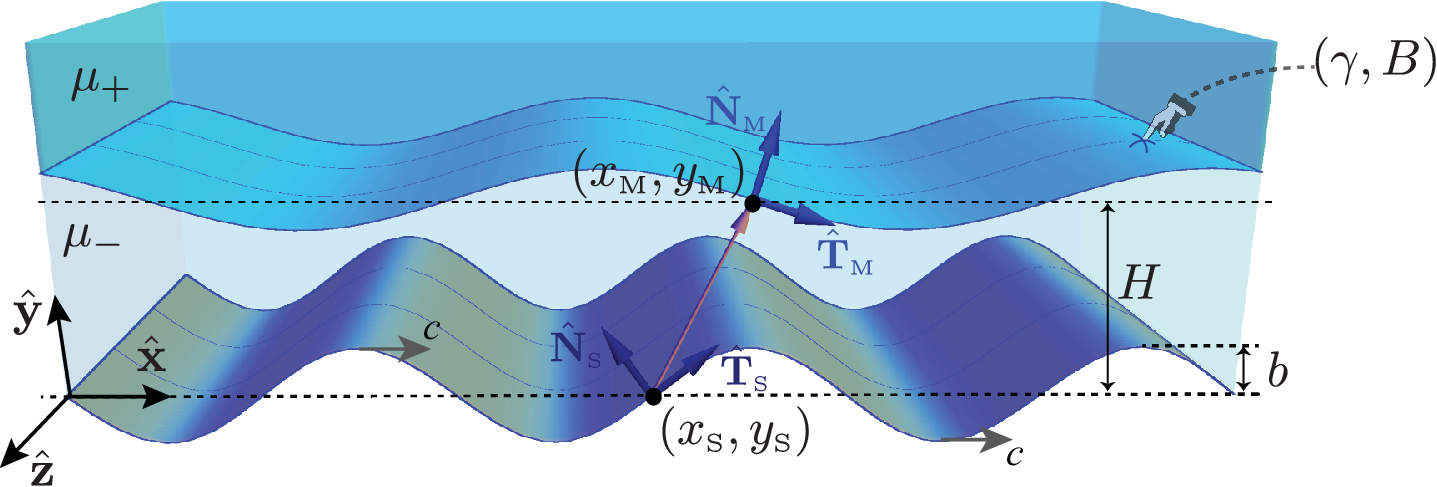
Figure 1 shows the setup of our model problem: a membrane with surface tension $\gamma$ and bending rigidity $B$ lies near a swimming sheet. The average separation between the sheet and the membrane is $H$, and the membrane separates two fluids with different viscosities, $\mu_{{\scriptscriptstyle\pm}}$. We disregard the space under the swimming sheet, since including a third fluid region introduces more complexity without adding any fundamentally new phenomena. We work in the frame of the swimmer. The material points on the swimming sheet have coordinates $(x_{\mbox{{\tiny S}}},y_{\mbox{{\tiny S}}})$, and the deformation of the swimmer is a prescribed transverse wave, with $x_{\mbox{{\tiny S}}}(x,t)=x$ and $y_{\mbox{{\tiny S}}}(x,t)=b\sin\left[k(x-ct)\right]$. The amplitude $b$ of the wave is assumed much smaller than the wavelength: $b\,k\ll 1$. Since $b$ is treated as infinitesimal, it is also always small compared to $H$. The material points on the sheet have velocity components given by $u_{\mbox{{\tiny S}}}={\partial x_{\mbox{{\tiny S}}}}/{\partial t}=0$ and $v_{\mbox{{\tiny S}}}={\partial y_{\mbox{{\tiny S}}}}/{\partial t}=-c\,kb\cos\left[k(x-ct)\right]$.

Given the deformation of the swimmer, the problem is to find the the velocity flow everywhere, the swimming speed of the sheet, and the shape and swimming speed of the membrane. Following Taylor [11], we expand in powers of $b\,k$ and find the swimming speed to leading order in $b\,k$; just as in Taylor’s case, the symmetry of the problem under $b\mapsto-b$ makes the swimming speed an even function of $b\,k$. The governing equations for the fluid are Stokes equations, $-\bm{\nabla}p_{{\scriptscriptstyle\pm}}+\mu_{{\scriptscriptstyle\pm}}\nabla^{2}\mathbf{v}_{{\scriptscriptstyle\pm}}=\bm{0}$ and $\bm{\nabla}\cdot\mathbf{v}_{{\scriptscriptstyle\pm}}=0$, where the $\pm$ subscript denotes the region above or below the membrane. The problem is two-dimensional since there is no dependence on $z$. The shape of the passive membrane is given by $(x_{\mbox{{\tiny M}}},y_{\mbox{{\tiny M}}})$, which are unknown functions of $x$ and $t$. At the surface of the swimmer and the membrane we impose no-slip boundary conditions,

Note that $x$ serves as a Lagrangian label for the swimmer and the membrane, with $x_{\mbox{{\tiny M}}}(x,t=0)=x$ when $b=0$.

Additional boundary conditions are required to determine the flow velocity and the deformation of the membrane. The balance of external viscous traction and internal elastic forces per unit area determines the shape of the membrane:

where $\kappa^{\prime\prime}$ is the second derivative of the curvature with respect to arclength [19]. In Eq. (2), $\hat{\mathbf{N}}_{\mbox{{\tiny M}}}$ is the upward-pointing unit normal of the membrane, $\hat{\mathbf{T}}_{\mbox{{\tiny M}}}$ is the unit tangent vector to the membrane, $\bm{\sigma}_{{\scriptscriptstyle\pm}}=-p_{{\scriptscriptstyle\pm}}\mathbb{I}+\mu_{{\scriptscriptstyle\pm}}\left[\bm{\nabla}\mathbf{v}_{{\scriptscriptstyle\pm}}+\left(\bm{\nabla}\mathbf{v}_{{\scriptscriptstyle\pm}}\right)^{T}\right]$ is the viscous stress with $p_{{\scriptscriptstyle\pm}}$ the pressure and $\mathbb{I}$ is the identity matrix. Note that the tangential stress in Eq. (2b) vanishes since we assume the tension $\gamma$ is uniform [19].

The force balance equations (2) imply that the $x$-component of force $\langle{\mathbf{f}}_{\mbox{{\tiny M}}}\rangle_{x}$ on the membrane is zero:

As we shall see below, the membrane translates in the $x$ direction even though the $x$-component of force vanishes; therefore, the membrane behaves as a passive swimmer.

Since the Reynolds number vanishes, the net force on the active swimmer vanishes, $\mathbf{F}=\int_{\mbox{{\tiny S}}}{\bm{\sigma}}_{{\scriptscriptstyle-}}\cdot\hat{\mathbf{N}}_{\mbox{{\tiny S}}}\,\mathrm{d}A=0$. In particular, the $x$-component of the hydrodynamic force per wavelength acting on the swimmer must also vanish:

We will use the notation $\langle\cdot\rangle$ to denote the average over a wavelength. We have listed all the boundary conditions required to find the flow velocity and the shape of the membrane. Note that if the deformation of the sheet leads to an average flow $\langle\hat{\mathbf{x}}\cdot\mathbf{v}_{{\scriptscriptstyle+}}(y\rightarrow\infty)\rangle$, then the sheet swims to the left with speed $V_{\mbox{{\tiny S}}}=\langle\hat{\mathbf{x}}\cdot\mathbf{v}_{{\scriptscriptstyle+}}(y\rightarrow\infty)\rangle$ in the laboratory frame. In the swimmer frame, the average speed of the membrane is ${\langle u_{\mbox{{\tiny M}}}\rangle}=(k/2\pi)\int_{0}^{2\pi/k}\mathrm{d}x\,\left.\partial{\psi}_{{\scriptscriptstyle\pm}}/\partial{y}\right|_{{x}_{\mbox{{\tiny M}}},{y}_{\mbox{{\tiny M}}}}$. Therefore, the membrane swims to the left with speed $V_{\mbox{{\tiny M}}}=V_{\mbox{{\tiny S}}}-\langle u_{\mbox{{\tiny M}}}\rangle$ in the laboratory frame.

Before solving the governing equations subject to the boundary conditions, it is convenient to cast them in dimensionless form by measuring length in units of $1/k$, rates in units of $c\,k$, and stress in units of $c\,k\,\mu_{{\scriptscriptstyle-}}$. These choices lead to the following natural dimensionless groups: the viscosity ratio $\mu_{r}\equiv\mu_{{\scriptscriptstyle+}}/\mu_{{\scriptscriptstyle-}}$, the capillary number ${C\!a}\equiv c\,\mu_{{\scriptscriptstyle-}}/\gamma$, and the Machin number ${M\!a}\equiv k^{2}B/\left(c\,\mu_{{\scriptscriptstyle-}}\right)$. Since the flow is incompressible and two-dimensional, it is also natural to work in terms of the stream function $\psi_{{\scriptscriptstyle\pm}}$, where $\mathbf{v}_{{\scriptscriptstyle\pm}}={\bm{\nabla}}\times(\hat{\mathbf{z}}\,\psi_{{\scriptscriptstyle\pm}})$. Taking the curl of the Stokes equations reveals that $\psi_{{\scriptscriptstyle\pm}}$ is biharmonic, $\nabla^{2}\psi_{{\scriptscriptstyle\pm}}=0$. Since we must simultaneously solve for the membrane shape using the force-balance conditions of Eq. (2a), we also solve for the pressure.

Expanding in powers of $b\,k$, and introducing the convenient variable $\zeta=x-t$, we have

where $\langle u_{\mbox{{\tiny M}}}\rangle=\sum_{n=1}^{\infty}(b\,k)^{n}U_{\mbox{{\tiny M}}}^{(n)}$. Because we work in the frame of the swimming organism, we require that $\partial\psi^{(2)}/\partial y$ approaches a constant and $\partial\psi^{(2)}/\partial x$ approaches zero as $y\rightarrow\infty$. Under these conditions, the general solution for the biharmonic equation is

where $\left\{A^{(m,n)}_{{\scriptscriptstyle\pm}},B^{(m,n)}_{{\scriptscriptstyle\pm}},C^{(m,n)}_{{\scriptscriptstyle\pm}},D^{(m,n)}_{{\scriptscriptstyle\pm}},E^{(m,n)}_{{\scriptscriptstyle-}},F^{(m,n)}_{{\scriptscriptstyle-}},G^{(m,n)}_{{\scriptscriptstyle-}},H^{(m,n)}_{{\scriptscriptstyle-}},u^{(1,n)}_{{\scriptscriptstyle\pm}},u^{(2,n)}_{{\scriptscriptstyle-}},u^{(3,n)}_{{\scriptscriptstyle-}}\right\}$ are functions of the dimensionless parameters $\{{C\!a},{M\!a},\mu_{r},H\}$ to be determined using the boundary conditions, Eqs. (1)–(4). A nonzero $u^{(1,n)}_{{\scriptscriptstyle-}}$ leads to a uniform flow in the region between the swimmer and the membrane, $u^{(2,n)}_{{\scriptscriptstyle-}}$ leads to pure shear flow, $u^{(3,n)}_{{\scriptscriptstyle-}}$ leads to parabolic flow, and $u^{(1,n)}_{{\scriptscriptstyle+}}$ leads to an average velocity of the fluid at infinity in the swimmer’s frame.

Note that the nonlinearity of the problem enters through the boundary conditions, which must be expanded to second order using the expressions in Eq.. 5b. Furthermore, we use the small-slope approximation to write $\kappa\approx-\partial^{2}y_{\mbox{{\tiny M}}}/\partial x^{2}$ and $\kappa^{\prime\prime}\approx-\partial^{4}y_{\mbox{{\tiny M}}}/\partial x^{4}$. We need only retain the $\mathcal{O}(b\,k)$ part of $\kappa$ and the bending force per unit area in Eq. (2a) because the corrections are $\mathcal{O}(b^{3}k^{3})$ and the swimming velocity turns out to be $\mathcal{O}(b^{2}k^{2})$. The first-order and second-order results are shown in appendices B and C, respectively.

As mentioned previously, there is no swimming velocity to first order in $b\,k$. However, the flow induced by the motion of the swimmer causes the membrane to have a first-order deformation. Solving (1c) and (2a) yields (see Appendix B)

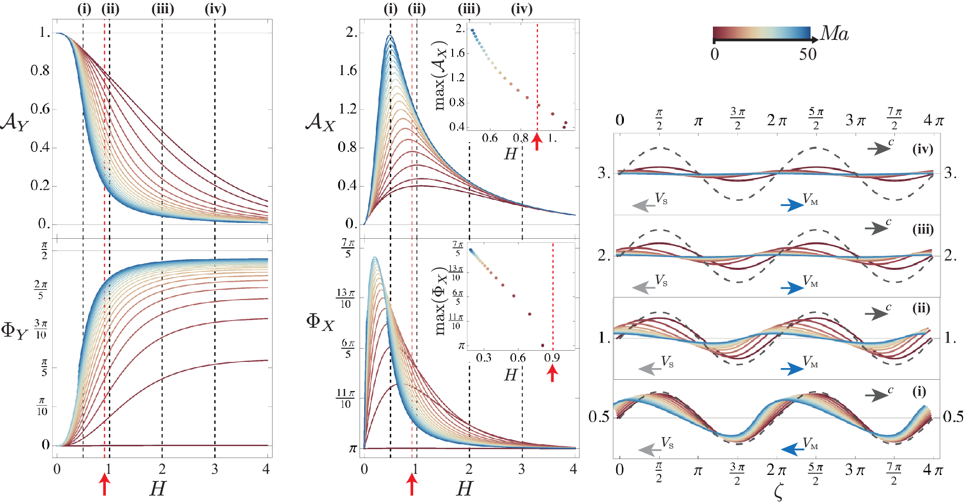
where the dependence of the amplitudes $\{\mathcal{A}_{X},\mathcal{A}_{Y}\}$ and phases $\{\Phi_{X},\Phi_{Y}\}$ on $M\!a$ and $H$ is shown in Fig. 2 (left and middle panels) for the case of $C\!a\rightarrow\infty$ and $\mu_{r}=\mu_{{\scriptscriptstyle+}}/\mu_{{\scriptscriptstyle-}}=1/2$. Figure 2 (right panel) also displays the shape of the membrane for various $M\!a$ for a few different values of $H$.

When the membrane is close to the swimmer, the waves induced on the membrane are mostly transverse, with an amplitude and phase close to that of the swimmer. As the separation $H$ increases, the transverse wave amplitude $\mathcal{A}_{Y}$ decreases while the longitudinal wave amplitude $\mathcal{A}_{X}$ increases, reaching a maximum at a value of $H$ that depends on $M\!a$. Eventually $\mathcal{A}_{X}$ also decreases with $H$ since the hydrodynamic interaction between the swimmer and membrane decreases with distance. Since there is no force preventing the membrane from translating, the induced waves cause the membrane to swim. We will see below that when the separation is small and transverse waves dominate, the membrane swims in the same direction as the swimmer. When the separation is large and longitudinal waves dominate, the membrane swims in the opposite direction as the swimmer, which is to be expected since sheet with purely longitudinal waves swims in the opposite direction as a sheet with purely transverse waves. We will see below that this explanation for swimming direction does not quantitatively predict the reversal in swimming direction of the membrane since it disregards the interplay of the phases of the wave, and since it does not completely account for the interaction between the membrane and the swimmer.

As validation, we have checked (see Appendix D) that our first-order stream function with ${M\!a}\rightarrow 0$, ${C\!a}\rightarrow\infty$, and $\mu_{r}\rightarrow 1$ agrees with Taylor’s result for swimming in an unbounded fluid [11], and that the stream function with ${M\!a}\rightarrow\infty$, ${C\!a}\rightarrow 0$, and $\mu_{r}\rightarrow\infty$ agrees with Reynolds’ [7] and Katz’s [8] results for swimming near a rigid wall.

We now turn to the second-order calculation (see Appendix C). Since we only seek time-averaged properties, we need only compute the unknowns $\left\{u^{(1,2)}_{{\scriptscriptstyle\pm}},u^{(2,2)}_{{\scriptscriptstyle-}},u^{(3,2)}_{{\scriptscriptstyle-}}\right\}$ and the average interface speed $U_{\mbox{{\tiny M}}}^{(2)}$. We impose the following boundary conditions: (i) the average of the no-slip condition over one spatial period (1a); (ii) the tangential force-balance condition on the membrane (2b); (iii) the force-free condition on the swimmer (4); and the no-slip condition at the membrane, which amounts to two conditions, (iv) below and (v) above the membrane. These five conditions are sufficient to determine the five unknowns.

For simplicity, here we consider a geometry in which either the flow beneath the swimmer is disregarded or the swimmer is moving in a symmetric channel. This simplification allows us to eliminate the contribution coming from pure shear, $u^{(2,2)}_{{\scriptscriptstyle-}}$. For an asymmetric channel, we must consider the flow below the swimmer, and the only other change is that the force-free condition on the swimmer will involve the fluid stresses from both sides of the swimmer, which leads to a nonzero shear flow. The force-free condition makes $u^{(3,2)}_{{\scriptscriptstyle-}}$ vanish whether or not the channel is symmetric. Translating back to the laboratory frame by subtracting off the average flow velocity at $y\rightarrow\infty$ yields (in dimensional form) the average fluid velocity within the gap between the swimmer and the membrane $V_{\mbox{\tiny pump}}=cb^{2}k^{2}\left(u^{(1,2)}_{{\scriptscriptstyle+}}-u^{(1,2)}_{{\scriptscriptstyle-}}\right)$, the membrane swimming speed $V_{\mbox{{\tiny M}}}=cb^{2}k^{2}\left(u^{(1,2)}_{{\scriptscriptstyle+}}-U_{\mbox{{\tiny M}}}^{(2)}\right)$, and the speed of the swimmer, $V_{\mbox{{\tiny S}}}=cb^{2}k^{2}\left(u^{(1,2)}_{{\scriptscriptstyle+}}-0\right)$. These expressions are too complicated to display here, but they simplify in the case of equal viscosities, $\mu_{r}=1$, for which we find $V_{\mbox{\tiny pump}}=0$, and

where $\Omega\equiv 4C\!a/(1+C\!aM\!a)$. Equation (8b) shows that the membrane speed vanishes at $H=1$ when $\mu_{r}=1$. From Fig. 3 we can see that the membrane speed vanishes at $H>1$ when $\mu_{r}>1$, and at $H<1$ when $\mu_{r}<1$ (indicated by the red dashed line). Even in the case of unequal viscosities we find that the swimming velocities depend on the material properties through $\Omega$. Thus, the form of $\Omega$ shows how the swimming speeds in the limit of zero capillary number and infinite Machin number are the same.

We now concentrate on the effects of bending rigidity by taking the limit ${C\!a}\rightarrow\infty$. The plots in Fig. 3 show the swimmer, pumping, and membrane speeds as a function of $H$, for the range $M\!a\in[0,50]$ and $\mu_{r}=1/2$, $\mu_{r}=1$, and $\mu_{r}=3/2$. First note that we recover Taylor’s results [11] when ${M\!a}\rightarrow 0$ and $\mu_{r}=1$; in this limit we find the swimming speed is independent of $H$ and there is no net flux of fluid entrained by the swimmer (Fig. 3, middle column). For all viscosity ratios, increasing the bending stiffness leads to enhancement of the swimmer’s speed and diminishment of the pumping and membrane speeds. The sign of the pumping speed is determined by the viscosity ratio alone, and is negative if $\mu_{r}<1$, zero if $\mu_{r}=1$, and positive if $\mu_{r}>1$. The swimmer develops its maximum speed in the limit where ${M\!a}\rightarrow\infty$, ${C\!a}\rightarrow 0$, and $\mu_{r}\rightarrow\infty$. This limit, shown in Fig. 3 as the dashed blue curve, is the hard-wall result derived previously in the literature [7, 8]. As mentioned previously, the sign of the membrane speed determined from the first-order results (7). A swimmer in an unbounded fluid [20] or in the presence of a wall [8] can swim backwards or forwards depending upon the competition between the longitudinal and transverse waves. Our results are also in agreement with this tendency:

where the new term $\mathcal{F}_{\mbox{\tiny int}}$ is a correction due to the elastic properties of the interface and the hydrodynamic interaction between the swimmer and the membrane. The dependence of $\mathcal{F}_{\mbox{\tiny int}}$ is shown in the insets in the third row of Fig. 3. Note that as $\mu_{r}$ gets larger, the amplitude of $\mathcal{F}_{\mbox{\tiny int}}$ decreases. For most values of $M\!a$, the peak of $\mathcal{F}_{\mbox{\tiny int}}$ lies to the left of the red dashed line. Therefore, this interaction tends to help the membrane swim in the same direction of the swimmer. The height in which the membrane speed changes sign, as shown in Fig. 3, depends on the viscosity ratio. Comparing the results in Figs. 2 and 3, we observe that positive membrane speeds are below the threshold (marked by the dashed, red, vertical line in Fig. 2) below which the maxima of $\Phi_{X}$ are located.

Figure 4 shows the speeds as a function of the membrane’s average height, in the limit ${M\!a}\rightarrow 0$ and ${C\!a}\rightarrow\infty$, for two special values of the viscosity ratio, (a) $\mu_{r}\rightarrow 0$ and (b) $\mu_{r}\approx 0.215$. These plots show that for a small enough viscosity ratio there is always a regime in which the swimmer has negative speed. In Fig. 4 (a), where $\mu_{{\scriptscriptstyle-}}/\mu_{{\scriptscriptstyle+}}\rightarrow\infty$, the swimmer has negative speed (swims in the direction of the propagating waves on the sheet) when $H\in[0.5,1.9]$ (dashed black vertical lines). Below $H\approx 1.7$ (dashed red vertical line indicated by the arrow), the membrane swims faster than the swimmer. The critical value of $\mu_{r}$ is $\mu_{r}\approx 0.215$ where the swimmer’s speed vanishes at $H=1$ (Fig. 4 (b)). It is a general feature of this system that whenever $\mu_{r}<1$, the pumping speed is always negative. The pumping is always positive when $\mu_{r}>1$.

To summarize, we have studied the problem of a swimming sheet near a deformable membrane with bending rigidity and a constant surface tension. Our main results are the swimming speed of the sheet as well as the deformation and swimming speed of the membrane. A distinctive feature of our problem that does not occur in the problem of a sheet swimming in unbounded fluid is that fluid is dragged along with or propelled backwards past the swimmer. Future work should lift some of the simplifying assumptions we have made, and examine finite-length swimmers with large amplitude deformations near flexible surfaces. Another generalization would be to consider swimming near an elastic half-space.

References

- [1] E. Lauga, W. R. DiLuzio, G. M. Whitesides, and H. A. Stone, “Swimming in circles: Motion of bacteria near solid boundaries,” Biophys. J. 90, 400–412 (2006).
- [2] H. Winet, G. S. Bernstein, and J. Head, “Observations on the response of human spermatozoa to gravity, boundaries and fluid shear,” Reproduction 70, 511–523 (1984).
- [3] K. Drescher, J. Dunkel, L. H. Cisneros, S. Ganguly, and R. E. Goldstein, “Fluid dynamics and noise in bacterial cell-cell and cell-surface scattering.” PNAS 108, 10940–5 (2011).
- [4] S. Boryshpolets, J. Cosson, V. Bondarenko, E. Gillies, M. Rodina, B. Dzyuba, and O. Linhart, “Different swimming behaviors of sterlet (Acipenser ruthenus) spermatozoa close to solid and free surfaces.” Theriogenology 79, 81–6 (2013).
- [5] S. S. Suarez, “How Do Sperm Get to the Egg? Bioengineering Expertise Needed!” Experim. Mech. 50, 1267–1274 (2009).
- [6] S. Lee, J. W. M. Bush, A. E. Hosoi, and E. Lauga, “Crawling beneath the free surface: Water snail locomotion,” Phys. of Fluids 20, 082106 (2008).
- [7] A. J. Reynolds, “The swimming of minute organisms,” J. of Fluid Mech. 23, 241 (1965).
- [8] D. F. Katz, “On the propulsion of micro-organisms near solid boundaries,” J. of Fluid Mech. 64, 33 (1974).
- [9] L. J. Fauci and A. McDonald, “Sperm motility in the presence of boundaries,” Bull. of Math. Biology 57, 679–699 (1995).
- [10] E. Lauga and T. R. Powers, “The hydrodynamics of swimming microorganisms,” Rep. on Prog. in Phys. 72, 096601 (2009).
- [11] G. I. Taylor, “Analysis of the Swimming of Microscopic Organisms,” Proc. of the Roy. Soc. A 209, 447–461 (1951).
- [12] A. A. Evans and E. Lauga, “Propulsion by passive filaments and active flagella near boundaries,” PRE 82, 041915 (2010).
- [13] R. Trouilloud, T. Yu, A. E. Hosoi, and E. Lauga, “Soft Swimming: Exploiting Deformable Interfaces for Low Reynolds Number Locomotion,” PRL 101, 1–4 (2008).
- [14] E. M. Purcell, “Life at low Reynolds number,” Am. J. of Phys. 45, 3 (1977).
- [15] J. C. Chrispell, L. J. Fauci, and M. Shelley, “An actuated elastic sheet interacting with passive and active structures in a viscoelastic fluid,” Phys. of Fluids 25, 013103 (2013).
- [16] R. Ledesma-Aguilar and J. M. Yeomans, “Enhanced motility of a microswimmer in an elastic tube,” arXiv:1303.7325 (2013).
- [17] C. Brennen and H. Winet, “Fluid Mechanics of Propulsion by Cilia and Flagella,” Ann. Rev. of Fluid Mech. 9, 339–398 (1977).
- [18] B. U. Felderhof, “Swimming and peristaltic pumping between two plane parallel walls,” J. of Phys. Cond. matter 21, 204106 (2009).
- [19] T. R. Powers, “Dynamics of filaments and membranes in a viscous fluid,” Rev. of Modern Phys. 82, 1607–1631 (2010).
- [20] J. R. Blake, “Infinite models for ciliary propulsion,” J. of Fluid Mech. 49, 209 (1971).