Pulling adsorbed self-avoiding walks from a surface
Abstract
We consider a self-avoiding walk model of polymer adsorption where the adsorbed polymer can be desorbed by the application of a force, concentrating on the case of the square lattice. Using series analysis methods we investigate the behaviour of the free energy of the system when there is an attractive potential with the surface and a force applied at the last vertex, normal to the surface, and extract the phase boundary between the ballistic and adsorbed phases. We believe this to be exact to graphical accuracy. We give precise estimates of the location of the transition from the free phase to the ballistic phase, which we find to be at and from the free phase to the adsorbed phase, which we estimate to be at . In addition we prove that the phase transition from the ballistic to the adsorbed phase is first order.
ARC Centre of Excellence for
Mathematics and Statistics of Complex Systems,
Department of Mathematics and Statistics,
The University of Melbourne, Victoria 3010, Australia
Department of Chemistry, University of Toronto, Toronto, Canada
1 Introduction
The theory of polymer adsorption [7, 21] has a long history [33, 35]. For linear polymers a variety of models have been considered including random walks [13, 33, 37], directed and partially directed walks [10, 22, 39] and self-avoiding walks [2, 3, 11, 15, 17, 20, 24]. In this paper we shall be concerned with the self-avoiding walk model for which there are a few rigorous results [15, 20] as well as extensive numerical investigations (see for instance [3, 11, 17, 24]).
The invention of micro-manipulation techniques such as atomic force microscopy (AFM) [40] which allow adsorbed polymer molecules to be pulled off a surface [16] has led to the development of theories of adsorbed polymers subject to a force [29, 31, 32, 36, 37]. Much of this work has focussed on random, directed and partially directed walk models but there has been some numerical work on the self-avoiding walk model [18, 29, 30] and a recent rigorous treatment [25] which establishes the existence of a phase boundary between an adsorbed phase and a ballistic phase when the force is applied normal to the surface. In this paper we use exact enumeration and series analysis techniques to identify this phase boundary for self-avoiding walks on the square lattice. We also make precise estimates of the critical points for adsorption with no force and for the transition to the ballistic phase with no surface interaction, and various relevant critical exponents. For a brief discussion of critical exponents appearing in this problem see [2] or [11].
2 Definitions and review of rigorous results
Consider the square lattice where the vertices have integer coordinates. We write , for the coordinates of the -th vertex of an -step self-avoiding walk on . The number of -step self-avoiding walks from the origin is denoted by . It is known that exists [14], where is the growth constant of self-avoiding walks on this lattice.
A positive walk is a self-avoiding walk on that starts at the origin and is constrained to have for all . The number of -step positive walks from the origin is denoted by . It is known that [38]. Vertices of a positive walk with are visits to the surface although, by convention, the vertex at the origin is not counted as a visit. We say that the walk has height if for the last vertex . The number of positive walks of -steps from the origin, with visits and height is denoted by . The corresponding partition function is
| (1) |
If is the energy associated with a visit and is the force applied at the last vertex, normal to the surface,
| (2) |
where is Boltzmann’s constant and is the absolute temperature. If no force is applied and the appropriate partition function is while if there is no interaction with the surface and the appropriate partition function is .
It is known [15] that the limit
| (3) |
exists and that is a convex function of . There exists a value of such that for and is strictly monotone increasing for . Therefore the free energy is non-analytic at [15] and this corresponds to the adsorption transition in the absence of a force. For , in the adsorbed phase,
| (4) |
while, for , . Here denotes expectation.
Similarly it is known [23] that the limit
| (5) |
exists and is a convex function of . There is a critical point such that for and is strictly monotone increasing for [23]. The critical point corresponds to a transition from a free phase where to a ballistic phase where
| (6) |
For the full two variable model it has recently been shown [25] that the limiting free energy
| (7) |
exists. is a convex function of and (i.e. convex as a surface) and
| (8) |
This implies that there is a free phase when and where and and a strictly monotone curve through the point separating two phases:
- 1.
an adsorbed phase when and , and
- 2.
a ballistic phase when .
Moreover, for the square lattice, is asymptotic to as .
3 Exact enumerations
The algorithm we use to enumerate self-avoiding walks (SAW) on the square lattice builds on the pioneering work of Enting [9] who enumerated square lattice self-avoiding polygons (SAP) using the finite lattice method. More specifically our algorithm is based in large part on the one devised by Conway, Enting and Guttmann [6] for the enumeration of SAWs. Many details of our algorithm can be found in [26]. All of the above transfer matrix (TM) algorithms are based on keeping track of the way partially constructed SAW are connected to the left of a cut-line bisecting the given finite lattice (rectangles in the case of the square lattice). Recently Clisby and Jensen [5] devised a new and more efficient implementation of the transfer-matrix algorithm for self-avoiding polygons. In that implementation we took a new approach and instead kept track of how a partially constructed SAP must connect up to the right of the cut-line. Jensen extended this approach to the enumeration of SAW [27]. Here we briefly describe how this algorithm can be amended to enumerate SAW configurations for the problem we study in this paper.
The first terms in the series for the SAW generating function can be calculated using transfer matrix techniques to count the number of walks in rectangles unit cells wide and cells long. Any walk spanning such a rectangle has a length of at least steps. By adding the contributions from all rectangles of width (where the choice of depends on available computational resources) and length the number of walks per vertex of an infinite lattice is obtained correctly up to length .


The basic idea of the algorithm can best be illustrated by considering the specific example of a SAW given in figure 1. Clearly any SAW is topologically equivalent to a line and therefore has exactly two end-points. If we cut the SAW by a vertical line as shown in figure 2 (the dashed line) we see that the SAW is broken into several pieces to the left and right of the cut-line. On either side of the cut-line we have a set of arcs connecting two edges on the cut-line and at most two line pieces connected to the end-points of the SAW. As we move the cut-line from left to right we prescribe what must happen in the future, that is how edges are to be connected to the right of the cut-line so as to form a valid SAW. Each end of an arc is assigned one of two labels depending on whether it is the lower or upper end of an arc. Any configuration along the cut-line can thus be represented by a set of edge states , where
| (9) |
If we read from the bottom to the top, the configuration or signature along the cut-lines of the SAW in figure 2 are, respectively, , , and . Since crossings are not permitted this encoding uniquely describes how the occupied edges are connected.
The most efficient implementation of the TM algorithm generally involves moving the cut-line in such a way as to build up the lattice vertex by vertex. The sum over all contributing graphs is calculated as the cut-line is moved through the lattice. For each configuration of occupied or empty edges along the intersection we maintain a generating function for partial walks with signature . In exact enumeration studies such as this is a truncated polynomial where is conjugate to the number of steps and to the number of visited vertices in the surface. In a TM update each source signature (before the boundary is moved) gives rise to a few new target signatures (after the move of the boundary line) as or 2 new edges are inserted with or 1 surface visits leading to the update . Once a signature has been processed it can be discarded.
Some minor changes to the basic algorithm described in [27] are required in order to enumerate the SAW configurations for the problem we study in this paper. Since we are moving the cut-line so as to add one vertex at a time we have complete control over the placement of the end-points of the SAW. In particular, grafting the SAW to the surface can be achieved by forcing the SAW to have a free end (the start-point) on the top of the rectangle. In enumerations of unrestricted SAW one can use symmetry to restrict the TM calculations to rectangles with and by counting contributions for rectangles with twice. The grafting of the start-point to the wall breaks the symmetry and we have to consider all rectangles with . The number of signatures one must consider grows exponentially with . Hence we must minimize the length of the cut-line to obtain an optimal algorithm. To achieve this the TM calculation on the set of rectangles is broken into two sub-sets with and , respectively. The calculations for the sub-set with is done as outlined above. In the calculations for the sub-set with the boundary line is chosen to be horizontal (rather than vertical) so it cuts across at most edges. Alternatively, one may view the calculation for the second sub-set as a TM algorithm for SAW with start-point on the left-most border of the rectangle. To keep track of the height of the end-point we simply specify that it must be placed in a row (or column) lattice-units from the surface and we then repeat the calculation for all the possible values of .
We calculated the number of SAW up to length . The calculation was performed in parallel using up to 16 processors, a maximum of some 40GB of memory and using a total of just under 6000 CPU hours (see [26] for details of the parallel algorithm).
4 Results
In this Section we describe the results from series analysis, chiefly using differential approximants [12]. We first discuss the -dependence of the free energy when there is no surface interaction, then the -dependence of the free energy when there is no applied force and finally the two variable free energy when there is both a surface interaction and a force.
4.1 No surface interaction.
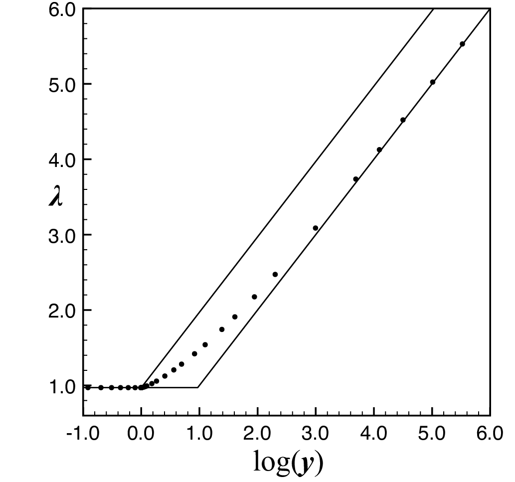
If we write
| (10) |
then will be singular at and, close to this singularity, is expected to behave as
| (11) |
where is a critical exponent whose value depends on the value of .
In table 1 below we give the results of an analysis of the series for various values of . The resulting estimates of the free energy are plotted in figure 3. The series were analysed using second and third order differential approximants [12]. At the series is well behaved and has critical point with exponent the exponent for terminally-attached self-avoiding walks (TASAW), as one expects [4]. For just below 1 the series are quite difficult to analyse. Estimates of are close to the known value For this is clearly evident from the analysis. And as gets smaller still, so that walks ending near to the surface are favoured, it is clear that the exponent is approaching as expected from the scaling law [1] This is the exponent appropriate to arches, often called loops in the literature. They are walks in the half-plane whose origin and end-point both lie in the surface. For the series really does suggest that with an exponent that looks very close to zero. For the approximants suggest that (so could be ) but there is another singularity very close by (at around ), and it is known that in such situations the estimate of the location, and exponent, is less trustworthy.
This sort of behaviour is typical of the situation in series analysis when one is in the vicinity of discontinuous change in the critical exponent. The only way a finite series – that is to say, a polynomial approximation to an infinite series – can mimic this discontinuity is by shifting the critical point slightly. So our conclusion is that the observed behaviour is consistent with the known result that for and that the exponent changes discontinuously from to as decreases below 1.
For the series are beautifully behaved, the singularity is clearly seen to be a simple pole, and we can provide 10 digit (or more) accuracy in estimates of the critical point. For we get the sort of behaviour we expect with a discontinuous change in exponent as we transition from an exponent to a simple pole.
So, in summary, it appears that for we have and exponent for we have and exponent and for we have monotonically decreasing as increases, and with a simple pole singularity.
An interesting and unexpected feature is that for all values of , the location of the antiferromagnetic singularity – that is to say, the singularity on the negative real axis, which for unconstrained SAWs is at – is unchanged at with exponent 11 1 To be precise, this singularity is less obvious for This can be understood from the fact that the radius of convergence of the series decreases as increases. The location of the anti-ferromagnetic singularity is located at a distance more than twice the radius of convergence when , so is increasingly difficult to detect. One would have to expect that it is there nonetheless..
A further bonus of this analysis is that the series analysis is exquisitely sensitive to the value of near This gives us a method for confirming that [19, 23]. From table 1, giving the results of an analysis of the series (see the second column of table 2) we find a value of the critical point very close to The value of is 0.379052277751, with uncertainty in the last digit only [5]. We can vary our estimate of until we get agreement with and this turns out to be at We know that , so combining our numerical results with this rigorous result, we conclude that . So it seems that for the exponent is given by and that this changes discontinuously to a simple pole for For the evidence strongly suggests that the exponent is given by
| Exponent | ||
|---|---|---|
| 0.4 | 0.379053 | 0.186 |
| 0.5 | 0.379052 | 0.186 |
| 0.6 | 0.379052 | 0.187 |
| 0.7 | 0.37905 | 0.195 |
| 0.8 | 0.37918 | 0.00 |
| 0.9 | 0.3792 | -0.3 |
| 0.99 | 0.37925 | -0.63 |
| 0.999 | 0.3790837 | -0.9328 |
| 0.9999 | 0.379055 | -0.950 |
| 0.99999 | 0.379052628 | -0.95296 |
| 0.999999 | 0.37905229 | -0.95307 |
| 1.0 | 0.37905225 | -0.95308 |
| 1.000001 | 0.37905221 | -0.95309 |
| 1.00001 | 0.37905188 | -0.95321 |
| 1.0001 | 0.3790488 | -0.9547 |
| 1.001 | 0.379019 | -0.970 |
| 1.01 | 0.37862 | -1.11 |
| 1.02 | 0.37804 | -1.137 |
| 1.04 | 0.37649 | -1.0 |
| 1.06 | 0.37463 | -0.99 |
| 1.08 | 0.37265 | -0.99 |
| 1.1 | 0.370564 | -1 |
| 1.2 | 0.3592886 | -1 |
| 1.3 | 0.3475682 | -1 |
| 1.5 | 0.3249328 | -1 |
| 1.75 | 0.2995547603 | -1 |
| 2.0 | 0.2775487 | -1 |
| 2.5 | 0.2418862105 | -1 |
| 3 | 0.214449855 | -1 |
| 4 | 0.1751070033 | -1 |
| 5 | 0.14820871438 | -1 |
| 7 | 0.1136573165016 | -1 |
| 10 | 0.084421281924 | -1 |
| 20 | 0.045635244067 | -1 |
| 40 | 0.02383593409377 | -1 |
| 60 | 0.01613729712 | -1 |
| 90 | 0.01087210691 | -1 |
| 150 | 0.00657951322 | -1 |
| 250 | 0.003968378456 | -1 |
4.2 No applied force.
Define the generating function
| (12) |
will be singular at and, close to this singularity, should behave as
| (13) |
where is a critical exponent whose value depends on the value of .

We have analysed the series corresponding to the “no force” situation. As in the previous “no interactions” case, we find that the series is exquisitely sensitive to the value of The best estimate [3] currently is with errors expected to be confined to the last quoted digit. That estimate is a comparatively recent result, which improved dramatically on pre-existing estimates, so improving on this, as we have done, is quite surprising. From table 2 below, we see from the second column that we find a value of the critical point very close to . We can vary our estimate of until we get agreement with and this turns out to be at with exponent which is satisfyingly close to the conjectured exact value [11, 2] where the superscript refers to the “special” transition that takes place right at the adsorption temperature [11]. As increases, we quickly see a simple pole emerging. So it seems that for the singularity is characterised by a (diverging) exponent and that this changes discontinuously to a simple pole for For the exponent is, as we would expect, given by If we analyse the series with and we can estimate the exponent We did this and found in agreement with the expected value [8]. In figure 4 we give our estimates of the free energy as a function of .
| Exponent | Exponent | |||
|---|---|---|---|---|
| 1.3 | 0.379052 | -0.952 | -0.37905 | 1.5 |
| 1.6 | 0.379058 | -0.96 | -0.3793 | 1 |
| 1.75 | 0.37910 | -1.31 | -0.37918 | 0.333 |
| 1.77559 | 0.37905237 | -1.4538 | -0.379050 | 0.256 |
| 1.775615 | 0.37905227 | -1.4539 | -0.379050 | 0.256 |
| 1.77564 | 0.37905217 | -1.4541 | -0.37905 | 0.256 |
| 1.775665 | 0.37905207 | -1.4542 | -0.37905 | 0.256 |
| 1.77569 | 0.37905197 | -1.4538 | -0.37905 | 0.256 |
| 1.8 | 0.37893 | -1.58 | -0.378885 | 0.189 |
| 2.0 | 0.37112 | -1.06 | -0.377 | -0.71 |
| 2.5 | 0.332682 | -1.0008 | -0.365065 | -0.517 |
| 2.75 | 0.3125387 | -0.999995 | -0.35806 | -0.5002 |
| 3.0 | 0.293630848 | -1 | -0.35106 | -0.5005 |
| 4.0 | 0.2329152160359 | -1 | -0.325298 | -0.499 |
| 5.0 | 0.191211527263626 | -1 | -0.30403 | -0.5005 |
| 6.0 | 0.16158981267578 | -1 | -0.28652 | -0.4995 |
| 7.5 | 0.130751327296498 | -1 | -0.26538 | -0.4994 |
| 10.0 | 0.0989240104593583 | -1 | -0.23912 | -0.4996 |
| 15.0 | 0.0663536371608435 | -1 | -0.20474 | -0.496 |
| 20.0 | 0.049869446447162 | -1 | -0.18249 | -0.503 |
| 40 | 0.0249840050794006 | -1 | -0.1367 | -0.6 |
| 60 | 0.01666196255 | -1 | ||
| 90 | 0.01110972448 | -1 | ||
| 150 | 0.0066663684218 | -1 | ||
| 250 | 0.00399993575 | -1 |
The behaviour of the antiferromagnetic singularity is different from that observed in the previous sub-section. For it seems stable at with an exponent that is likely to be exactly as for the case above. For however, the anti-ferromagnetic critical point monotonically decreases as increases for and (conjecturally) has a square root singularity. At it looks more like a fourth root branch point, but a zero, not a divergence.22 2 The estimate of the singularity location is not very precise, so it’s entirely possible that the exponent is not exactly but some fraction of approximately similar value.
4.3 Phase diagram calculation

In order to locate the phase boundary between the adsorbed and ballistic phases, in the -plane, we make use of (8). is equal to throughout the adsorbed phase and to throughout the ballistic phase. The phase boundary between the adsorbed and ballistic phases is the locus of points where . For a given value of we calculated as in Section 4.2 and then found the value of such that by interpolating the results for found in Section 4.1. More precisely, from table 1 we calculated by using the program Eureqa [34] on columns 1 and 2 of table 1. As a relevant technical detail, in actual implementation it is desirable to minimize the variation of the parameters as much as possible. Accordingly, we sought a fit to the functional form where In this way we found an interpolation formula, which we used by inserting the values from table 2, so as to obtain the values corresponding to the values in table 2. In this way we obtained the results shown in table 3.
As a check, we also calculated points on the curve starting with a given value of and reversing the procedure. More precisely, from table 2 we calculated also by using Eureqa on columns 1 and 2 of table 2, and found an interpolation formula. We obtained a further set of values by substituting the values from table 1, so as to obtain the values corresponding to the values in table 1. In this way we obtained the results shown in table 4.
Combining the data in these two tables results in the phase boundary shown in figure 5 where we have plotted the data from table 3 as red circles and the data from table 4 as blue diamonds. The close agreement between the two independent analyses implies that the results are accurate to at least graphical accuracy.. The curve passes through the point , is strictly monotone increasing and asymptotic to , as shown in [25]. It is interesting to note that the curve is not concave.
We can switch to physical variables (force and temperature) using (2). Without much loss of generality we can set and work in units where . The corresponding phase boundary in the force-temperature plane is given in figure 6. Notice that the force at zero is 1 and the limiting slope at is zero, as predicted in [25]. The curve is monotone decreasing as increases, with no re-entrance. See for instance [25, 30, 36] for further discussion. The force-temperature curve is in semi-quantitative agreement with an earlier numerical study by Mishra et al [30], but is substantially more precise.

| 1.775615 | 0.37905227 | 1 |
|---|---|---|
| 1.77569 | 0.37905197 | 1.0001 |
| 1.8 | 0.37893 | 1.0030 |
| 2.0 | 0.37112 | 1.0953 |
| 2.5 | 0.332682 | 1.4293 |
| 2.75 | 0.3125387 | 1.6174 |
| 3.0 | 0.293630848 | 1.8137 |
| 4.0 | 0.23291521603 | 2.6510 |
| 5.0 | 0.19121152726 | 3.5399 |
| 6.0 | 0.16158981268 | 4.4592 |
| 7.5 | 0.13075132730 | 5.8729 |
| 10.0 | 0.09892401046 | 8.2816 |
| 15.0 | 0.06635363716 | 13.189 |
| 20.0 | 0.04986944645 | 18.146 |
| 40 | 0.02498400508 | 38.118 |
| 60 | 0.01666196255 | 58.136 |
| 90 | 0.01110972448 | 88.145 |
| 150 | 0.00666636842 | 148.00 |
| 250 | 0.00399993575 | 247.18 |
| 1.0 | 0.37905225 | 1.775615 |
|---|---|---|
| 1.001 | 0.379019 | 1.7854 |
| 1.01 | 0.37862 | 1.8220 |
| 1.02 | 0.37804 | 1.8456 |
| 1.04 | 0.37649 | 1.8915 |
| 1.06 | 0.37463 | 1.9347 |
| 1.08 | 0.37265 | 1.9733 |
| 1.1 | 0.370564 | 2.0092 |
| 1.2 | 0.3592886 | 2.1693 |
| 1.3 | 0.3475682 | 2.3161 |
| 1.5 | 0.3249328 | 2.5934 |
| 1.75 | 0.2995547603 | 2.9206 |
| 2.0 | 0.277548710 | 3.2329 |
| 2.5 | 0.2418862105 | 3.8287 |
| 3 | 0.214449855 | 4.4003 |
| 4 | 0.1751070033 | 5.5029 |
| 5 | 0.14820871438 | 6.5747 |
| 7 | 0.11365731650 | 8.6708 |
| 10 | 0.08442128192 | 11.757 |
| 20 | 0.04563524407 | 21.876 |
| 40 | 0.02383593409 | 41.923 |
| 60 | 0.01666196255 | 61.912 |
| 90 | 0.01110972448 | 91.864 |
| 150 | 0.00666636842 | 151.74 |
| 250 | 0.00399993575 | 251.50 |
5 The behaviour and nature of the phase transition on the phase boundary.
It is possible to use the results of [25] to prove that the phase transition from the ballistic to the adsorbed phase is first order. We state this as a theorem.
Theorem 1.
The free energy is not differentiable at the phase boundary between the ballistic and adsorbed phases, except perhaps at the point .
Proof: There is a monotone strictly increasing curve in the -plane, through the point , corresponding to the phase boundary between the ballistic and adsorbed phases. In the ballistic phase and in the adsorbed phase . The free energy is a monotone increasing function of , convex in . It therefore has left and right derivatives at every value of . Throughout the adsorbed phase the left and right derivatives of are positive. Consider a line of fixed . The free energy for and for . For . For the right derivative of with respect to is positive. Therefore the left and right derivatives of with respect to at are not equal and the free energy is not differentiable. ∎
However it is still of interest to determine how the free energy behaves as we approach the phase boundary. We “know” the location of the phase boundary from the results reported in the previous section, at least to graphical accuracy. That is to say, with an accuracy of three to four significant digits. At the phase boundary, we also know the value of the radius of convergence, from the data above. So, by way of example, at the phase boundary is at If we analyse the series at this point, (recall this just means substituting the required values of and into the three-variable generating function we have, which produces a one-variable generating function, where the expansion variable is conjugate to the length of the walk) we find the critical point is at with an exponent of This is exactly the same value of found at though at the exponent is a simple pole.
As we increase we see exactly the same behaviour as observed in section 1 that allowed us to identify That is to say, there is a variation in the criticial point and critical exponent as the approximants struggle to cope with a discontinuous exponent change. So at the pair is estimated to be This large error in the exponent estimate is a signature that the analysis method is struggling. At we find and at which is our best estimate of the intersection of the line with the phase boundary, we find for the critical point and exponent Note that this value of the critical point is exactly that found when and which is well below the phase boundary.
Suggestive as this is, we note that the value of chosen is rather close to the point (a bicritical point, see [28]), where the behaviour is different, and may still have an effect on the convergence rate of the series. So we take another example, when which is well away from the point . At the critical point is and the exponent is a simple pole. The phase boundary point at is estimated to be at Analysis of the series at that point gives rather confirming the double pole. The location is slightly different from that observed at but that is likely ascribable to the estimate of on the phase boundary being slightly in error. Indeed, if we repeat the analysis with we find and the exponent estimate is which is rather convincing evidence for a double pole!
So we find that at (or very near to and below) the phase boundary, the series are well-converged, give the estimates of the critical point we expect, and display a double pole singularity. Near to the phase boundary, the estimates are very variable, and behave in exactly the same way as did the series analysed in section 4, with the approximants seemingly struggling to cope with a discontinuous change in the critical exponent.
It is instructive to consider the simpler case of directed positive walks. We discuss two cases:
- 1.
Positive walks with step set and , which we refer to loosely as Dyck paths, and
- 2.
Positive walks with step set , and , which we refer to loosely as Motzkin paths.
It is straightforward to solve each of these models exactly, though we don’t give the details here. They each show three phases (a free phase, an adsorbed phase and a ballistic phase). There is a phase boundary between the adsorbed and ballistic phases and in both cases these phase boundaries are concave in the -plane. In the Motzkin path case the phase boundary is asymptotic to while in the Dyck path case it is asymptotic to , because a maximum of half the vertices can be in the surface. In each case the singularity in both the adsorbed and ballistic phases is a simple pole so the generating function has both of these singularities though one is dominant in the adsorbed phase and the other is dominant in the ballistic phase. On the phase boundary between the adsorbed and ballistic phases these two singularities are equal resulting in a double pole, just as observed numerically for the case of SAWs.
6 Discussion
We have considered a self-avoiding walk model of polymer adsorption at an impenetrable surface where
- 1.
the walk is terminally attached to the surface,
- 2.
the walk interacts with the surface with an attractive potential, and
- 3.
the walk is subject to a force applied normal to the surface at the last vertex of the walk.
For the square lattice we have used series analysis techniques to investigate the phases and phase boundaries for the system. There are three phases, a free phase where the walk is desorbed but not ballistic, an adsorbed phase where the walk is adsorbed at the surface and a ballistic phase where the walk is desorbed but ballistic. We have located the phase boundaries and proved that the phase transition from the adsorbed to the ballistic phase is first order. In addition we have very precise values for the critical points for adsorption without a force and for the free to ballistic transition with no surface interaction.
Acknowledgements
The authors would like to acknowledge helpful conversations with Enzo Orlandini, and help with the preparation of the data files by Jason Whyte. This research was partially supported by NSERC of Canada. The computations for this work were supported by an award to IJ under the Merit Allocation Scheme on the NCI National Facility at the Australian National University. IJ and AJG were supported under the Australian Research Council’s Discovery Projects funding scheme by the grants DP120101593 and DP120100939 respectively. We thank Cornell Creative Machines Lab for making available the program Eurequa [34].
References
- [1] Barber M N, Guttmann A J, Middlemiss K M, Torrie G M and Whittington S G 1978 J. Phys. A: Math. Gen. 11 1833-42
- [2] Batchelor M T and Yung C M 1995 Phys. Rev. Lett. 74 2026-2029
- [3] Beaton N R, Guttmann A J and Jensen I 2012 J. Phys. A: Math. Theor. 45 055208
- [4] Cardy J L 1984 Nucl. Phys. B 240 514-532
- [5] Clisby N and Jensen I 2012 J. Phys. A: Math. Theor. 45 115202
- [6] Conway A R, Enting I G and Guttmann A J 1993 J. Phys. A: Math. Gen. 26 1519–1534
- [7] De’Bell K and Lookman T 1993 Rev. Mod. Phys. 65 87-113
- [8] Duplantier B and Saleur H 1986, Phys. Rev. Lett. 57 3179-3182
- [9] Enting I G 1980 J. Phys. A: Math. Gen. 13 3713–3722
- [10] Forgacs G, Privman V and Frisch H L 1989 J. Chem. Phys. 90 3339-3345
- [11] Guim I and Burkhardt T W 1989 J. Phys. A: Math. Gen. 22 1131-1140
- [12] Guttmann A J and Jensen I, in Polygons, Polyominoes and Polycubes, ed. A J Guttmann, Lecture Notes in Physics 775 Springer, The Netherlands, (2009)
- [13] Hammersley J M 1982 J. Appl. Prob. 19 327-331
- [14] Hammersley J M and Morton K W 1954 J. Roy. Stat. Soc. B 16 23-38
- [15] Hammersley J M, Torrie G M and Whittington S G 1982 J. Phys. A: Math. Gen. 15 539-571
- [16] Haupt B J, Ennis J and Sevick E M 1999 Langmuir 15 3886-389
- [17] Hegger R and Grassberger P 1994 J. Phys. A: Math. Gen. 27 4069-4081
- [18] Iliev G K, Orlandini E and Whittington S G 2013 J. Phys. A: Math. Theor. 46 055001
- [19] Ioffe D and Velenik Y, Ballistic phase of self-interacting random walks, 2008, Analysis and Stochastics of Growth Processes and Interface Models ed P Morters, R Moser, M Penrose, H Schwetlick and J Zimmer Oxford: Oxford University Press) pp 55-79
- [20] Janse van Rensburg E J 1998 J. Phys. A: Math. Gen. 31 8295-8306
- [21] Janse van Rensburg E J 2000 The Statistical Mechanics of Interacting Walks, Polygons, Animals and Vesicles. Oxford University Press.
- [22] Janse van Rensburg E J 2003 J. Phys. A: Math. Gen. 36 R11-R61
- [23] Janse van Rensburg E J, Orlandini E, Tesi M C and Whittington S G 2009 J. Stat. Mech. P07014
- [24] Janse van Rensburg E J and Rechnitzer A 2004 J. Phys. A: Math. Gen. 37 6875-6898
- [25] Janse van Rensburg E J and Whittington S G 2013 J. Phys. A: Math. Theor. 46 435003
- [26] Jensen I 2004 J. Phys. A: Math. Gen. 37 5503–5524
- [27] Jensen I 2013 A new transfer-matrix algorithm for exact enumerations: self-avoiding walks on the square lattice, arXiv 1309.6709
- [28] Klushin L I, Skvortsov A M and Gorbunov A A 1997 Phys. Rev. E 56 1511-1521
- [29] Krawczyk J, Owczarek A L, Prellberg T and Rechnitzer A 2005 J. Stat. Mech. P05008
- [30] Mishra P K, Kumar S and Singh Y 2005 Europhys. Letters 69 102-108
- [31] Orlandini E, Tesi M C and Whittington S G 1999 J. Phys. A: Math. Gen. 32 469-477
- [32] Owczarek A L 2010 J. Phys. A: Math. Theor. 43 225002
- [33] Rubin R J 1965 J. Chem. Phys. 43 2392-2407
- [34] Schmidt M, Lipson H 2009 Science, 324 no. 5923, 81 - 85
- [35] Silberberg A 1962 J. Phys. Chem. 66 1872-1883
- [36] Skvortsov A M, Klushin L I, Fleer G J and Leermakers F A M 2009 J. Chem. Phys. 130 174704
- [37] Skvortsov A M, Klushin L I, Polotsky A A and Binder K 2012 Phys. Rev. E 85 031803
- [38] Whittington S G 1975 J. Chem. Phys. 63 779-785
- [39] Whittington S G 1998 J. Phys. A: Math. Gen. 31 8797-8803
- [40] Zhang W and Zhang X 2003 Prog. Polym. Sci. 28 1271-1295