跳到论文正文
W Papers独立论文阅读器 arXiv:1309.6727 论文正文 计算阅读时间 · 0%
引用这篇论文根据当前论文元数据生成,正式投稿前建议核对。


License: arXiv.org perpetual non-exclusive license
arXiv:1309.6727v2 [cs.IT] 26 May 2016

Genie Tree and Degrees of Freedom of the Symmetric MIMO Interfering Broadcast Channel

Tingting Liu    Member, IEEE    Chenyang Yang    Senior Member, IEEE ††thanks: T. Liu and C. Yang are with the School of Electronics and Information Engineering, Beihang University, Beijing 100191, China. (E-mail: {ttliu,cyyang}@buaa.edu.cn)
Abstract

In this paper, we study the information theoretic maximal degrees of freedom (DoF) for the symmetric multi-input-multi-output (MIMO) interfering broadcast channel (IBC) with arbitrary antenna configurations. For the GG-cell KK-user M×NM\times N MIMO-IBC network, we find that the information theoretic maximal DoF per user are related to three DoF bounds: 1) the decomposition DoF bound dDecom=M​N/(M+K​N)d^{\mathrm{Decom}}=MN/(M+KN), a lower-bound of linear interference alignment (IA) with infinite time/frequency extensions (called asymptotic IA); 2) the proper DoF bound dProper=(M+N)/(G​K+1)d^{\mathrm{Proper}}=(M+N)/(GK+1), an upper-bound of linear IA without time/frequency extensions (called linear IA); and 3) the quantity DoF bound dQuand^{\mathrm{Quan}}, a zigzag piecewise linear function of MM and NN. The whole region of M/NM/N can be divided into two regions, Region I: ℛI={M/N|dProper<dDecom}\mathcal{R}^{\mathrm{I}}=\{M/N|d^{\mathrm{Proper}}<d^{\mathrm{Decom}}\} and Region II: ℛII={M/N|dProper≥dDecom}\mathcal{R}^{\mathrm{II}}=\{M/N|d^{\mathrm{Proper}}\geq d^{\mathrm{Decom}}\}. Specifically, for most configurations in Region I, the information theoretic maximal DoF are the decomposition DoF bound and can be achieved by the asymptotic IA. For all configurations in Region II, the information theoretic maximal DoF are the quantity DoF bound and can be achieved by the linear IA.

To obtain the tight upper-bound, we propose a unified way to construct genies, where the genies help each base station or user resolve the maximal number of interference. According to the feature that the designed genies with the same dimension can derive identical DoF upper-bound, we convert the information theoretic DoF upper-bound problem into a linear algebra problem and obtain the closed-form DoF upper-bound expression. Moreover, we develop a non-iterative linear IA transceiver to achieve the DoF upper-bound for the networks with antenna configurations in Region II, which means that the derived DoF upper-bound is tightest. The basic principles to derive the DoF upper-bound and design the linear IA transceiver to achieve the DoF upper-bound can be extended into general asymmetric networks.

Index Terms: 
Interference alignment (IA), interfering broadcast channel (IBC), degrees of freedom (DoF), genie tree, irresolvable and resolvable inter-cell interferences (ICIs)

I Introduction

Inter-cell interference (ICI) is a bottleneck of improving the sum capacity of multi-cell networks, especially when multi-input-multi-output (MIMO) techniques are used. The degrees of freedom (DoF) can reflect the potential of interference networks, which are the first-order approximation of sum capacity at high signal-to-noise ratio (SNR) regime [2, 1]. Recently, significant research efforts have been devoted to find the DoF for MIMO interference channel (MIMO-IC) [2, 1, 3, 4, 5, 6, 7, 9, 8], MIMO interfering broadcast channel (MIMO-IBC) [10, 11, 12], and MIMO interfering multiple access (MIMO-IMAC) [13] networks.

For the symmetric GG-cell M×NM\times N MIMO-IC network where each base station (BS) and each mobile station (MS) have MM and NN antennas, respectively, when the channels are time/frequency varying and M=NM=N, the information theoretic maximal DoF per user are M/2M/2. This implies that the sum DoF can linearly increase with GG, and the performance of the interference network is not interference-limited [3]. Encouraged by such a promising result, many recent works strive to analyze the information theoretic maximal DoF for the MIMO-IC [1, 4, 3, 2, 5, 6, 7] and MIMO-IBC [10, 11, 12] networks with various antenna configurations and devise interference management techniques to achieve the information theoretic maximal DoF.

For the two-cell MIMO-IC network, the information theoretic maximal DoF were obtained with all antenna configurations in [2] and can be achieved by the linear interference alignment (IA). For the symmetric three-cell M×NM\times N MIMO-IC network, the information theoretic maximal DoF were obtained as a piecewise linear function of MM and NN in [1] and achievable by the linear IA. For the symmetric two-cell KK-user M×NM\times N MIMO-IBC network where K=2,3K=2,3, the information theoretic maximal DoF were obtained with all antenna configurations in [10] and achievable by the linear IA. These results show that when G=2G=2, K=1,2,3K=1,2,3 and G=3G=3, K=1K=1, the linear IA can achieve the information theoretic maximal DoF.

However, for the networks where G=2,K≥4G=2,~K\geq 4, G=3,K≥2G=3,~K\geq 2, and G≥4,K≥1G\geq 4,~K\geq 1, the information theoretic maximal DoF were only obtained with special configurations.11 1 The configurations are summarized in Table II. For many antenna configurations in these networks, the information theoretic maximal DoF cannot be achieved by the linear IA, but can be achieved by the asymptotic IA in [3].

Considering that infinite time/frequency extensions of asymptotic IA are not viable for practical networks, many studies investigated the maximal DoF achieved by the linear IA. For the MIMO-IC network with constant coefficients, the feasible conditions of linear IA, called IA conditions for short, were derived in [15]. The IA conditions contain a class of rank constraints to receive the desired signals and a class of zero-forcing constraints to eliminate all ICIs. A proper condition was first proposed in [14], which requires that the number of variables to cancel the ICIs is greater than or equal to the number of ICIs. When the channels in the MIMO-IC network are generic (i.e., drawn from a continuous probability distribution), the authors in [16, 17] proved that the proper condition is a necessary condition for the feasibility of linear IA. The proper condition was proved to be sufficient for two cases: 1) M=NM=N in [16] and 2) either MM or NN is divisible by the number of data streams per user dd [17]. The study in [8] investigated the sufficient conditions of linear IA feasibility for the asymmetric MIMO-IC. In [9], the authors developed a polynomial complexity test that allows a complete characterization of the achievable DoF region by the linear IA for the symmetric MIMO-IC with arbitrary antenna configuration. For the MIMO-IBC network with generic channels, the proper condition was proved to be necessary in [18, 19] and to be sufficient for two cases: 1) M=N+(K−1)​dM=N+(K-1)d by extending the result in [16] and 2) either MM or NN is divisible by dd in [19]. For general cases, these results did not answer when the proper condition is sufficient and when the linear IA can achieve the information theoretic maximal DoF.

So far, the following questions are still open for general MIMO-IC and MIMO-IBC networks:

  1. 1.

    What are the information theoretic maximal DoF?

  2. 2.

    How to derive the information theoretic maximal DoF? How to design IA transceiver to achieve the information theoretic maximal DoF?

  3. 3.

    Why some linear IA transceivers that satisfy the proper condition are infeasible?

This paper strives to answer these questions. The main contributions are summarized as follows,

  1. 1.

    We obtain the information theoretic maximal DoF for the symmetric GG-cell KK-user M×NM\times N MIMO-IBC network. The whole region of M/NM/N is divided into two parts, Region I and Region II. For most configurations in Region I, the information theoretic maximal DoF are M​N/(M+K​N)MN/(M+KN), which are achievable by the asymptotic IA.22 2 This study considers the asymptotic IA proposed in [3], which is a linear IA with infinite time/frequency extensions. For all configurations in Region II, the information theoretic maximal DoF are the piecewise linearly function of MM and NN, which are achievable by the linear IA.33 3 This study considers the linear IA discussed in [14], which is a linear IA with no time/frequency extensions. The finite spatial extensions [1] are allowed to avoid the loss of DoF caused by restricting the value of DoF to an integer.

  2. 2.

    We provide a unified method to construct genies to derive the tight DoF upper-bound for the networks with general configurations, which is different from the methods in [7, 1] where different ways were developed for different configurations. By dividing the ICIs into resolvable ICIs and irresolvable ICIs, we construct the genie to assist each BS or user to resolve the maximal number of irresolvable ICIs in order to derive the tightest upper-bound. By using the feature that identical DoF upper-bound can be obtained from the genies with the same dimension, we convert the information theoretic DoF upper-bound problem into a linear algebra problem to obtain the closed-form DoF upper-bound expression. According to the structure of genie tree, we obtain the tightest DoF upper-bound and develop a non-iterative linear IA transceiver to achieve the DoF upper-bound with all antenna configurations in Region II.

  3. 3.

    We find that there exists a kind of ICIs44 4 The ICIs are irreducible ICIs defined in [19]. that must be solely eliminated by the BSs or the users but cannot be jointly eliminated by the BSs and users. The proper condition does not ensure the system to provide enough antennas to eliminate this kind of ICIs, which explains why some linear IA transceivers are proper but infeasible.

The basic principles of constructing the genie tree to derive the DoF upper-bound and design the feasible linear IA transceiver can be extended into asymmetric MIMO-IC, MIMO-IBC and MIMO-IMAC networks with general antenna configurations.

The rest of the paper is organized as follows. We describe the system model in Section II. We present the information theoretic maximal DoF in Section III and prove the results in Sections IV and V, respectively. Conclusions are given in the last section.

Notations: Transpose, Hermitian transpose and expectation are represented by (⋅)T(\cdot)^{T}, (⋅)H(\cdot)^{H}, and 𝔼​{⋅}\mathbb{E}\{\cdot\}, respectively. diag​{⋅}\mathrm{diag}\{\cdot\} is a block diagonal matrix. For the vector 𝒙\boldsymbol{x}, 𝒙⁡(i)\boldsymbol{x}(i) denotes its iith variable, and 𝒙⁡(i:j)\boldsymbol{x}(i:j) denotes a row vector obtained from its iith to jjth variables. Similarly, for the matrix 𝑿\boldsymbol{X}, 𝑿⁡(i)\boldsymbol{X}(i) denotes its iith column vector, and 𝑿⁡(i:j)\boldsymbol{X}(i:j) denotes a matrix obtained from its iith to jjth columns.

II System Model and Definition

II-A System Model

Consider a GG-cell multiuser MIMO network where GG BSs each with MM antennas serves KK users each with NN antennas. All channel state information is assumed available at all nodes. In information theory terminology, this is a symmetric MIMO-IBC network, denoted as the GG-cell KK-user M×NM\times N MIMO-IBC network.

The information theoretic maximal DoF for the MIMO-IBC network are equal to those for the MIMO-IMAC network. Nevertheless, since the signal models of both MIMO-IBC and MIMO-IMAC networks are necessary to derive the DoF, we provide the signal models of both networks.

In the MIMO-IMAC network, the received signals of the jjth BS (denoted by BSj) can be expressed as

𝒚j=\displaystyle\boldsymbol{y}_{j}= ∑i=1G∑k=1K𝑯j,ik​𝒙ik+𝒏j\displaystyle\sum_{i=1}^{G}\sum_{k=1}^{K}\boldsymbol{H}_{j,i_{k}}\boldsymbol{x}_{i_{k}}+\boldsymbol{n}_{j} (1)

where 𝒙ik∈ℂN×1\boldsymbol{x}_{i_{k}}\in\mathbb{C}^{N\times 1} is a vector of transmit signals of the kkth MS in the iith cell (denoted by MSik{}_{i_{k}}), 𝑯j,ik∈ℂM×N\boldsymbol{H}_{j,i_{k}}\in\mathbb{C}^{M\times N} is the channel matrix from MSik{}_{i_{k}} to BSj, whose elements are independent and identically distributed (i.i.d.) random variables with a continuous distribution, and 𝒏j∈ℂM×1\boldsymbol{n}_{j}\in\mathbb{C}^{M\times 1} is the zero-mean additive white Gaussian noise of BSj with covariance matrix 𝔼⁡{𝒏j​𝒏jH}=σn2​𝑰M\mathbb{E}\left\{\boldsymbol{n}_{j}\boldsymbol{n}_{j}^{H}\right\}=\sigma_{n}^{2}\boldsymbol{I}_{M}.

In the MIMO-IBC network, the received signals of MSik{}_{i_{k}} can be expressed as

𝒚ik=\displaystyle\boldsymbol{y}_{i_{k}}= ∑j=1G𝑯j,ikT​𝒙j+𝒏ik\displaystyle\sum_{j=1}^{G}\boldsymbol{H}_{j,i_{k}}^{T}\boldsymbol{x}_{j}+\boldsymbol{n}_{i_{k}} (2)

where 𝒙j∈ℂM×1\boldsymbol{x}_{j}\in\mathbb{C}^{M\times 1} is a vector of transmit signals of BSj, and 𝒏ik∈ℂN×1\boldsymbol{n}_{i_{k}}\in\mathbb{C}^{N\times 1} is the zero-mean additive white Gaussian noise of MSik{}_{i_{k}} with covariance matrix 𝔼⁡{𝒏ik​𝒏ikH}=σn2​𝑰N\mathbb{E}\left\{\boldsymbol{n}_{i_{k}}\boldsymbol{n}_{i_{k}}^{H}\right\}=\sigma_{n}^{2}\boldsymbol{I}_{N}.

Definition 1

The DoF per user with finite spatial extensions are defined as [1]

d⁡(M,N)≜maxm∈ℤ+⁡{d¯​(m​M,m​N)m}\displaystyle d(M,N)\triangleq\max_{m\in\mathbb{Z}^{+}}\left\{\frac{\bar{d}(mM,mN)}{m}\right\} (3)

where d¯​(M,N)≜limγ→∞R⁡(γ)/log⁡γ\bar{d}(M,N)\triangleq\lim_{\gamma\rightarrow\infty}{R(\gamma)}/{\log\gamma} are the DoF per user without spatial extensions, R⁡(γ)R(\gamma) is the achievable rate per user for the given SNR γ\gamma, and mm is a finite integer and ℤ+\mathbb{Z}^{+} is the set of positive integers. It means that the DoF of m​d​(M,N)m{d}(M,N) are achievable for each user when each BS and each user are equipped with m​MmM and m​NmN antennas. With finite spatial extensions, the value of DoF per user is not necessary to be an integer, which avoids the loss of DoF due to rounding.

For notational simplicity, in the sequel we omit M,NM,N and use dd to denote the DoF per user as well as the number of data streams able to be supported for each user.

II-B Related Notions

In the forthcoming analysis, we will show that the expression and derivation of information theoretic maximal DoF are related to the notions of generalized continued fraction sequence [21] and tree in graph theory [22]. For readers’ convenience, we first briefly introduce these notions.

II-B1 Continued Fraction

Definition 2

A generalized continued fraction sequence is a sequence in the form [21]

xn=β0+α1β1+α2β2+α3⋯+αnβn,∀n∈ℤ+\displaystyle x_{n}=\beta_{0}+\cfrac{\alpha_{1}}{\beta_{1}+\cfrac{\alpha_{2}}{\beta_{2}+\cfrac{\alpha_{3}}{\cdots+\cfrac{\alpha_{n}}{\beta_{n}}}}},\forall n\in\mathbb{Z}^{+} (4)

The generalized continue fraction sequence has the following properties [21].

Property 1

The generalized continue fraction sequence in (4) can be expressed as a ratio of a generalized Fibonacci sequence-pair, i.e.,

xn=qn/pn\displaystyle x_{n}={q_{n}}/{p_{n}} (5)

where {qn,pn}\{q_{n},p_{n}\} is the generalized Fibonacci sequence-pair satisfying {q−1,p−1}={1,0}\{q_{-1},p_{-1}\}=\{1,0\}, {q0,p0}={β0,1}\{q_{0},p_{0}\}=\{\beta_{0},1\}, and

{qn,pn}=(βn​qn−1+αn​qn−2,βn​pn−1+αn​pn−2),∀n∈ℤ+\displaystyle\{q_{n},p_{n}\}=(\beta_{n}q_{n-1}+\alpha_{n}q_{n-2},\beta_{n}p_{n-1}+\alpha_{n}p_{n-2}),\forall n\in\mathbb{Z}^{+}
Property 2

The generalized continue fraction sequence in (4) can be expressed in the form of series as

xn=β0+∑m=1n−1(−1)m​∏i=1m−1αipm​pm+1,∀n∈ℤ+\displaystyle x_{n}=\beta_{0}+\sum_{m=1}^{n-1}\frac{(-1)^{m}\prod_{i=1}^{m-1}\alpha_{i}}{p_{m}p_{m+1}},\forall n\in\mathbb{Z}^{+} (6)

II-B2 Tree

In graph theory [22], a tree is a connected graph without cycles, as shown in Fig. 1. A rooted tree is a tree with a designated vertex called the root, e.g., vertex rr. In a rooted tree, the depth of vertex vv is the distance from the root to the vertex. The height is the greatest depth. The height of the tree in Fig. 1 is two. If vertex vv immediately precedes vertex ww on the path from the root to ww, then vv is the parent of ww and ww is the child of vv. A leaf is any vertex having no children, e.g., vertexes ww, yy, and zz. A branch is a subtree without the root. A branch with the greatest height is called the maximal branch. In Fig. 1, vertexes xx, yy, and zz constitute a maximal branch.

Refer to caption
Fig. 1: Basic notions of rooted tree in graph theory.

III Information Theoretic Maximal DoF

In this section, we first present and compare several DoF bounds for symmetric MIMO-IBC networks. Then, we present the information theoretic maximal DoF to be proved later and show the connection with existing results in the literature.

III-A DoF Bounds

III-A1 Decomposition DoF Bound

For the GG-cell M×NM\times N MIMO-IC, the decomposition DoF bound was derived as dDecom=M​N/(M+N)d^{\mathrm{Decom}}=MN/(M+N). It was a lower-bound of DoF per user introduced in [5] and achievable by the asymptotic IA through decomposing the antennas of both BSs and users.

Using the similar way of decomposing the antennas of the BSs, a GG-cell KK-user M×NM\times N MIMO-IBC network can be decomposed to a G​KGK-cell M/K×NM/K\times N MIMO-IC network.55 5 Since we consider finite spatial extensions, the number of antennas is no necessary to be an integer. Then, the decomposition DoF bound for the symmetric MIMO-IBC network can be obtain as

dDecom=M/K⋅NM/K+N=M​NM+K​N\displaystyle d^{\mathrm{Decom}}=\frac{M/K\cdot N}{M/K+N}=\frac{MN}{M+KN} (7)

which is achievable by the asymptotic IA designed for the MIMO-IC network in [3].

From (7), we know that the achievable DoF per user are independent of the number of cells GG. It implies that the achieved sum DoF of the network can linearly increase with GG.

III-A2 Proper DoF Bound

In [14], a proper condition was proposed, which has been proved to be necessary for the feasibility of linear IA in the MIMO-IC [16, 17] and MIMO-IBC networks [19], when the channels are generic. For the symmetric MIMO-IBC network, the proper condition was [19]

M+N≥(G​K+1)​d\displaystyle M+N\geq(GK+1)d (8)

We call the upper-bound of DoF per user obtained from the proper condition the proper DoF bound. From (8), the proper DoF bound is obtained as

dProper=M+NG​K+1\displaystyle d^{\mathrm{Proper}}=\frac{M+N}{GK+1} (9)

Then, the upper-bound of the sum DoF is G​K​(M+N)/(G​K+1)GK(M+N)/(GK+1). As GG or KK increases, the sum DoF are bounded by M+NM+N.

Fig. 2: Comparison of three DoF bounds for the symmetric MIMO-IBC.

In Fig. 2, we compare the decomposition DoF bound and the proper DoF bound with different values of M/NM/N. For some values of M/NM/N, the decomposition DoF bound is greater than the proper DoF bound, while for others, the decomposition DoF bound is less than the proper DoF bound. For easy exposition, we divide the whole region of M/NM/N into two parts, called Region I and Region II and denoted by ℛI\mathcal{R}^{\mathrm{I}} and ℛII\mathcal{R}^{\mathrm{II}}, respectively. Specifically, we define the two regions as

ℛI\displaystyle\mathcal{R}^{\mathrm{I}} ≜{M/N|dProper<dDecom}\displaystyle\triangleq\left\{M/N|d^{\mathrm{Proper}}<d^{\mathrm{Decom}}\right\} (10a)
ℛII\displaystyle\mathcal{R}^{\mathrm{II}} ≜{M/N|dProper≥dDecom}\displaystyle\triangleq\left\{M/N|d^{\mathrm{Proper}}\geq d^{\mathrm{Decom}}\right\} (10b)

By substituting (7) and (9) into (10), it is not difficult to express Regions I and II as

ℛI\displaystyle\mathcal{R}^{\mathrm{I}} =(ξB,ξA),∀{K≥4,G=2K≥1,G≥3\displaystyle=\left(\xi^{\mathrm{B}},\xi^{\mathrm{A}}\right),~\forall\left\{\begin{array}[]{l}K\geq 4,G=2\\ K\geq 1,G\geq 3\end{array}\right.
ℛII\displaystyle\mathcal{R}^{\mathrm{II}} ={(0,∞),∀K≤3,G=2(0,ξB]∪[ξA,∞),otherwise.\displaystyle=\left\{\begin{array}[]{ll}\left(0,\infty\right),&~\forall K\leq 3,G=2\\ \left(0,\xi^{\mathrm{B}}\right]\cup\left[\xi^{\mathrm{A}},\infty\right),&~\mathrm{otherwise.}\\ \end{array}\right.

where ξA=((G−1)​K+(G−1)2​K2−4​K)/2\xi^{\mathrm{A}}=((G-1)K+\sqrt{(G-1)^{2}K^{2}-4K})/2 and ξB=((G−1)​K−(G−1)2​K2−4​K)/2\xi^{\mathrm{B}}=((G-1)K-\sqrt{(G-1)^{2}K^{2}-4K})/2.

III-A3 Quantity DoF Bound

In the forthcoming analysis, we will provide a DoF bound that is a piecewise linear function of MM and NN and prove that the DoF bound is the information theoretical maximal DoF. When G=3G=3 and K=1K=1, the DoF bound reduces to the quantity DoF introduced in [1]. Therefore, we call it the quantity DoF bound.

For the symmetric MIMO-IBC network, the quantity DoF bound to be proved later is expressed as

dQuan={min⁡{MK+CnA,N1+KCn−1A},∀M/N∈ℛnAmin⁡{MK+Cn−1B,N1+KCnB},∀M/N∈ℛnB\displaystyle d^{\mathrm{Quan}}=\left\{\begin{array}[]{ll}\min\left\{\frac{M}{K+C_{n}^{\mathrm{A}}},\frac{N}{1+\frac{K}{C_{n-1}^{\mathrm{A}}}}\right\},&~\forall M/N\in\mathcal{R}^{\mathrm{A}}_{n}\\ \min\left\{\frac{M}{K+C_{n-1}^{\mathrm{B}}},\frac{N}{1+\frac{K}{C_{n}^{\mathrm{B}}}}\right\},&~\forall M/N\in\mathcal{R}^{\mathrm{B}}_{n}\end{array}\right.

where ℛnA≜[CnA,Cn−1A)\mathcal{R}^{\mathrm{A}}_{n}\triangleq\left[C_{n}^{\mathrm{A}},C_{n-1}^{\mathrm{A}}\right), ℛnB≜(Cn−1B,CnB]\mathcal{R}^{\mathrm{B}}_{n}\triangleq\left(C_{n-1}^{\mathrm{B}},C_{n}^{\mathrm{B}}\right], C0A=∞C_{0}^{\mathrm{A}}=\infty, C0B=0C_{0}^{\mathrm{B}}=0, and

CnA≜\displaystyle C_{n}^{\mathrm{A}}\triangleq (G−1)​K−K/Cn−1A\displaystyle(G-1)K-{K}/{C_{n-1}^{\mathrm{A}}} (14a)
CnB≜\displaystyle C_{n}^{\mathrm{B}}\triangleq 1G−1−Cn−1B/K\displaystyle\frac{1}{G-1-{C_{n-1}^{\mathrm{B}}}/{K}} (14b)

satisfying CnA,CnB≥0,∀n∈ℤ+,n≤nmaxC_{n}^{\mathrm{A}},C_{n}^{\mathrm{B}}\geq 0,~\forall n\in\mathbb{Z}^{+},n\leq n^{\max} with

nmax={2,∀G=2,K=13,∀G=2,K=25,∀G=2,K=3∞,otherwise.\displaystyle n^{\max}=\left\{\begin{array}[]{ll}2,&\forall G=2,K=1\\ 3,&\forall G=2,K=2\\ 5,&\forall G=2,K=3\\ \infty,&\mathrm{otherwise.}\end{array}\right.

To understand the properties of the quantity DoF bound, we show several values of {CnA}\{C_{n}^{\mathrm{A}}\} and {CnB}\{C_{n}^{\mathrm{B}}\} in Table III.

TABLE I: Values of {CnA}\{C_{n}^{\mathrm{A}}\} and {CnB}\{C_{n}^{\mathrm{B}}\}
nn CnAC_{n}^{\mathrm{A}} CnBC_{n}^{\mathrm{B}}
0 ∞\infty 00
1 (G−1)​K(G-1)K 1G−1\cfrac{1}{G-1}
2 (G−1)​K−1G−1(G-1)K-\cfrac{1}{G-1} 1G−1−1(G−1)​K\cfrac{1}{G-1-\cfrac{1}{(G-1)K}}
3 (G−1)​K−1G−1−1(G−1)​K(G-1)K-\cfrac{1}{G-1-\cfrac{1}{(G-1)K}} 1G−1−1(G−1)​K−1G−1\cfrac{1}{G-1-\cfrac{1}{(G-1)K-\cfrac{1}{G-1}}}
⋮ ⋮ ⋮

From Table III, we can see that CnAC_{n}^{\mathrm{A}} and CnBC_{n}^{\mathrm{B}}, ∀n∈ℤ+,n≤nmax\forall n\in\mathbb{Z}^{+},n\leq n^{\max} are the generalized continued fraction sequences as follows,

CnA\displaystyle C_{n}^{\mathrm{A}} =(G−1)​K¯0−1(G−1)​K¯1−1⋯1(G−1)​K¯n−1\displaystyle=(G-1)\bar{K}_{0}-\cfrac{1}{(G-1)\bar{K}_{1}-\cfrac{1}{\cdots\cfrac{1}{(G-1)\bar{K}_{n-1}}}} (19a)
CnB\displaystyle C_{n}^{\mathrm{B}} =1(G−1)​K¯1−1(G−1)​K¯2−1⋯1(G−1)​K¯n\displaystyle=\cfrac{1}{(G-1)\bar{K}_{1}-\cfrac{1}{(G-1)\bar{K}_{2}-\cfrac{1}{\cdots\cfrac{1}{(G-1)\bar{K}_{n}}}}} (19b)

where

K¯n≜{K,∀n​is​even.1,∀n​is​odd.\displaystyle\bar{K}_{n}\triangleq\left\{\begin{array}[]{cc}K,&~\forall n\mathrm{~is~even.}\\ 1,&~\forall n\mathrm{~is~odd.}\end{array}\right.

According to Property 1, CnAC_{n}^{\mathrm{A}} and CnBC_{n}^{\mathrm{B}}, ∀n∈ℤ+,n≤nmax\forall n\in\mathbb{Z}^{+},n\leq n^{\max} can be rewritten as the ratios of generalized Fibonacci sequence-pairs, i.e.,

CnA=qnA/pnA,CnB=qnB/pnB\displaystyle C_{n}^{\mathrm{A}}={q_{n}^{\mathrm{A}}}/{p_{n}^{\mathrm{A}}},~C_{n}^{\mathrm{B}}={q_{n}^{\mathrm{B}}}/{p_{n}^{\mathrm{B}}} (22)

where (pnA,qnA)\left(p_{n}^{\mathrm{A}},q_{n}^{\mathrm{A}}\right) and (pnB,qnB)\left(p_{n}^{\mathrm{B}},q_{n}^{\mathrm{B}}\right) are the generalized Fibonacci sequence-pairs satisfying (p0A,q0A)=(0,1)\left(p_{0}^{\mathrm{A}},q_{0}^{\mathrm{A}}\right)=(0,1), (p−1A,q−1A)=(−1,0)\left(p_{-1}^{\mathrm{A}},q_{-1}^{\mathrm{A}}\right)=(-1,0), (p0B,q0B)=(1,0)\left(p_{0}^{\mathrm{B}},q_{0}^{\mathrm{B}}\right)=(1,0), (p−1B,q−1B)=(0,−1)\left(p_{-1}^{\mathrm{B}},q_{-1}^{\mathrm{B}}\right)=(0,-1), and

{pnA≜(G−1)​K¯n−1​pn−1A−pn−2AqnA≜(G−1)​K¯n−1​qn−1A−qn−2A\displaystyle\left\{\begin{array}[]{ll}p_{n}^{\mathrm{A}}&\triangleq(G-1)\bar{K}_{n-1}p_{n-1}^{\mathrm{A}}-p_{n-2}^{\mathrm{A}}\\ q_{n}^{\mathrm{A}}&\triangleq(G-1)\bar{K}_{n-1}q_{n-1}^{\mathrm{A}}-q_{n-2}^{\mathrm{A}}\\ \end{array}\right.
{pnB≜(G−1)​K¯n​pn−1B−pn−2BqnB≜(G−1)​K¯n​qn−1B−qn−2B\displaystyle\left\{\begin{array}[]{ll}p_{n}^{\mathrm{B}}&\triangleq(G-1)\bar{K}_{n}p_{n-1}^{\mathrm{B}}-p_{n-2}^{\mathrm{B}}\\ q_{n}^{\mathrm{B}}&\triangleq(G-1)\bar{K}_{n}q_{n-1}^{\mathrm{B}}-q_{n-2}^{\mathrm{B}}\\ \end{array}\right.

satisfying pnA,qnA,pnB,qnA>0,∀n∈ℤ+,n≤nmaxp_{n}^{\mathrm{A}},q_{n}^{\mathrm{A}},p_{n}^{\mathrm{B}},q_{n}^{\mathrm{A}}>0,~\forall n\in\mathbb{Z}^{+},n\leq n^{\max}.

According to Property 2, CnAC_{n}^{\mathrm{A}} and CnBC_{n}^{\mathrm{B}}, ∀n∈ℤ+,n≤nmax\forall n\in\mathbb{Z}^{+},n\leq n^{\max} can be rewritten as the series as follows,

CnA\displaystyle C_{n}^{\mathrm{A}} =(G−1)​K−∑m=1n−11pmA​pm+1A\displaystyle=(G-1)K-\sum_{m=1}^{n-1}\frac{1}{p_{m}^{\mathrm{A}}p_{m+1}^{\mathrm{A}}} (24a)
CnB\displaystyle C_{n}^{\mathrm{B}} =∑m=1n−11pmB​pm+1B\displaystyle=\sum_{m=1}^{n-1}\frac{1}{p_{m}^{\mathrm{B}}p_{m+1}^{\mathrm{B}}} (24b)

Since pmA,pmB≥0,∀m∈ℤ+,m≤nmaxp_{m}^{\mathrm{A}},p_{m}^{\mathrm{B}}\geq 0,~\forall m\in\mathbb{Z}^{+},~m\leq n^{\max}, {CnA}\left\{C_{n}^{\mathrm{A}}\right\} is a monotonically decreasing sequence, whereas {CnB}\left\{C_{n}^{\mathrm{B}}\right\} is a monotonically increasing sequence.

In (III-A3), dQuand^{\mathrm{Quan}} is a piecewise function defined in M/N∈ℛA∪ℛBM/N\in\mathcal{R}^{\mathrm{A}}\cup\mathcal{R}^{\mathrm{B}}, where ℛA≜∪n=1nmaxℛAn\mathcal{R}^{\mathrm{A}}\triangleq\cup_{n=1}^{n^{\max}}\mathcal{R}^{\mathrm{A}}_{n} and ℛB≜∪n=1nmaxℛBn\mathcal{R}^{\mathrm{B}}\triangleq\cup_{n=1}^{n^{\max}}\mathcal{R}^{\mathrm{B}}_{n}, respectively. According to the derivation in Appendices and , we obtain the feature of dQuand^{\mathrm{Quan}} in the following lemmas.

Lemma 1

ℛA\mathcal{R}^{\mathrm{A}} and ℛB\mathcal{R}^{\mathrm{B}} are two subregions of Region II, i.e.,

ℛII=ℛA∪ℛB\displaystyle\mathcal{R}^{\mathrm{II}}=\mathcal{R}^{\mathrm{A}}\cup\mathcal{R}^{\mathrm{B}} (25)

Lemma 1 suggests that the quantity DoF bound dQuand^{\mathrm{Quan}} is a piecewise function defined in Region II. We call the two subregions of of Region II as Region II-A and Region II-B and denote them by ℛII−A\mathcal{R}^{\mathrm{II-A}} and ℛII−B\mathcal{R}^{\mathrm{II-B}} in the following.

Lemma 2

The quantity DoF bound dQuand^{\mathrm{Quan}} satisfies

dDecom≤dQuan≤dProper,\displaystyle d^{\mathrm{Decom}}\leq d^{\mathrm{Quan}}\leq d^{\mathrm{Proper}}, ∀M/N∈ℛII\displaystyle~\forall M/N\in\mathcal{R}^{\mathrm{II}} (26)

and

dQuan\displaystyle d^{\mathrm{Quan}} =dDecom,∀M/N∈{CnA,CnB}\displaystyle=d^{\mathrm{Decom}},~\forall M/N\in\{C_{n}^{\mathrm{A}},C_{n}^{\mathrm{B}}\} (27a)
dQuan\displaystyle d^{\mathrm{Quan}} =dProper,∀M/N∈{DnA,DnB}\displaystyle=d^{\mathrm{Proper}},~\forall M/N\in\{D_{n}^{\mathrm{A}},D_{n}^{\mathrm{B}}\} (27b)

where

DnA=K+Cn+1A1+K/CnA,DnB=K+CnB1+K/Cn+1B\displaystyle D_{n}^{\mathrm{A}}=\frac{K+C_{n+1}^{\mathrm{A}}}{1+K/C_{n}^{\mathrm{A}}},~D_{n}^{\mathrm{B}}=\frac{K+C_{n}^{\mathrm{B}}}{1+K/C_{n+1}^{\mathrm{B}}} (28)

As shown in Fig. 2, in Region II, the quantity DoF bound is a zigzag curve between the proper DoF bound and the decomposition DoF bound.

III-B Information Theoretic Maximal DoF

Theorem 1 (DoF Upper-bound)

For the GG-cell KK-user M×NM\times N MIMO-IBC network, the DoF per user are bounded by

d\displaystyle d ≤dDecom,∀M/N∈ℛI∩𝒬\displaystyle\leq d^{\mathrm{Decom}},~\forall M/N\in\mathcal{R}^{\mathrm{I}}\cap\mathcal{Q}~ (29a)
d\displaystyle d ≤dQuan,∀M/N∈ℛII\displaystyle\leq d^{\mathrm{Quan}},~\forall M/N\in\mathcal{R}^{\mathrm{II}} (29b)

where

𝒬≜{q~l,nα/p~l,nα},α=A,B,n∈ℤ+\displaystyle\mathcal{Q}\triangleq\{\tilde{q}_{l,n}^{\alpha}/\tilde{p}_{l,n}^{\alpha}\},~\alpha=\mathrm{A},~\mathrm{B},~n\in\mathbb{Z}^{+} (30)

when n=2​m−1,α=An=2m-1,~\alpha=A or n=2​m,α=Bn=2m,~\alpha=B, ∀m∈ℤ+\forall m\in\mathbb{Z}^{+}, l=jl=j,66 6 It means that q~l,nα,p~l,nα\tilde{q}_{l,n}^{\alpha},~\tilde{p}_{l,n}^{\alpha} in (30) are the parameters of BSj. when n=2​m,α=An=2m,~\alpha=A or n=2​m−1,α=Bn=2m-1,~\alpha=B, l=ikl=i_{k}.77 7 It indicates that q~l,nα,p~l,nα\tilde{q}_{l,n}^{\alpha},~\tilde{p}_{l,n}^{\alpha} in (30) are the parameters of MSik{}_{i_{k}} Here, (p~l,nA,q~l,nA)(\tilde{p}_{l,n}^{\mathrm{A}},\tilde{q}_{l,n}^{\mathrm{A}}) and (p~l,nB,q~l,nB)(\tilde{p}_{l,n}^{\mathrm{B}},\tilde{q}_{l,n}^{\mathrm{B}}) are the generalized Fibonacci sequence-pairs satisfying (p~l,0A,q~l,0A)=(0,1)(\tilde{p}_{l,0}^{\mathrm{A}},\tilde{q}_{l,0}^{\mathrm{A}})=(0,1), (p~l,−1A,q~l,−1A)=(−1,0)(\tilde{p}_{l,-1}^{\mathrm{A}},\tilde{q}_{l,-1}^{\mathrm{A}})=(-1,0), (p~l,0B,q~l,0B)=(1,0)(\tilde{p}_{l,0}^{\mathrm{B}},\tilde{q}_{l,0}^{\mathrm{B}})=(1,0), (p~l,−1B,q~l,−1B)=(0,−1)(\tilde{p}_{l,-1}^{\mathrm{B}},\tilde{q}_{l,-1}^{\mathrm{B}})=(0,-1), and

p~l,nα\displaystyle\tilde{p}_{l,n}^{\alpha} ≜∑r∈ℐl,nαp~r,n−1α−p~l,n−2α\displaystyle\triangleq\sum_{r\in\mathcal{I}_{l,n}^{\alpha}}\tilde{p}_{r,n-1}^{\alpha}-\tilde{p}_{l,n-2}^{\alpha} (31a)
q~l,nα\displaystyle\tilde{q}_{l,n}^{\alpha} ≜∑r∈ℐl,nαq~r,n−1α−q~l,n−2α\displaystyle\triangleq\sum_{r\in\mathcal{I}_{l,n}^{\alpha}}\tilde{q}_{r,n-1}^{\alpha}-\tilde{q}_{l,n-2}^{\alpha} (31b)

satisfying p~l,nα,q~l,nα>0\tilde{p}_{l,n}^{\alpha},\tilde{q}_{l,n}^{\alpha}>0, ∀n∈ℤ+\forall n\in\mathbb{Z}^{+}, and ℐl,nA,ℐl,nB⊆ℐl\mathcal{I}_{l,n}^{\mathrm{A}},\mathcal{I}_{l,n}^{\mathrm{B}}\subseteq\mathcal{I}_{l} satisfy

∑r∈ℐl,nAq~r,n−1A−2​q~l,n−2A∑r∈ℐl,nAp~r,n−1A−2​p~l,n−2A≤MN\displaystyle\frac{\sum_{r\in\mathcal{I}_{l,n}^{\mathrm{A}}}\tilde{q}_{r,n-1}^{\mathrm{A}}-2\tilde{q}_{l,n-2}^{\mathrm{A}}}{\sum_{r\in\mathcal{I}_{l,n}^{\mathrm{A}}}\tilde{p}_{r,n-1}^{\mathrm{A}}-2\tilde{p}_{l,n-2}^{\mathrm{A}}}\leq\frac{M}{N} (32a)
∑r∈ℐl,nBq~r,n−1B−2​q~l,n−2B∑r∈ℐl,nBp~r,n−1B−2​p~l,n−2B≥MN\displaystyle\frac{\sum_{r\in\mathcal{I}_{l,n}^{\mathrm{B}}}\tilde{q}_{r,n-1}^{\mathrm{B}}-2\tilde{q}_{l,n-2}^{\mathrm{B}}}{\sum_{r\in\mathcal{I}_{l,n}^{\mathrm{B}}}\tilde{p}_{r,n-1}^{\mathrm{B}}-2\tilde{p}_{l,n-2}^{\mathrm{B}}}\geq\frac{M}{N} (32b)

ℐik={j|j≠i,j⊆{1,⋯,G}}\mathcal{I}_{i_{k}}=\{j|j\neq i,~j\subseteq\{1,\cdots,G\}\} and ℐj={ik|i≠j,i⊆{1,⋯,G},k⊆{1,⋯,K}}\mathcal{I}_{j}=\{i_{k}|i\neq j,~i\subseteq\{1,\cdots,G\},~k\subseteq\{1,\cdots,K\}\} denote the set of interfering BSs for MSik{}_{i_{k}} and the set of interfering users for BSik{}_{i_{k}}, respectively.

In Theorem 1, (29a) indicates that the decomposition DoF is the DoF upper-bound for most configurations in Region I,88 8 We have studies the property of 𝒬\mathcal{Q} and found that 𝒬\mathcal{Q} includes the most antenna configurations in Region I. Due to the page limitation, we will provide the detailed proof in our future work. and (29b) means that the quantity DoF is the DoF upper-bound for all configurations in Region II.

Theorem 2 (Achievable DoF)

For the GG-cell KK-user M×NM\times N MIMO-IBC network, the achievable DoF per user satisfy

d\displaystyle d ≥dDecom,∀M/N∈ℛI\displaystyle\geq d^{\mathrm{Decom}},~\forall M/N\in\mathcal{R}^{\mathrm{I}} (33a)
d\displaystyle d ≥dQuan,∀M/N∈ℛII\displaystyle\geq d^{\mathrm{Quan}},~\forall M/N\in\mathcal{R}^{\mathrm{II}} (33b)

In Region I, the DoF of dDecomd^{\mathrm{Decom}} are achievable by the asymptotic IA. In Region II, the DoF of dQuand^{\mathrm{Quan}} are achievable by the linear IA.

From Theorems 1 and 2, we can obtain the information theoretic maximal DoF immediately.

Corollary 1 (Information Theoretic Maximal DoF)

For the GG-cell KK-user M×NM\times N MIMO-IBC network, the information theoretic maximal DoF per user are

dmax\displaystyle d^{\max} =dDecom,∀M/N∈ℛI∩𝒬\displaystyle=d^{\mathrm{Decom}},~\forall M/N\in\mathcal{R}^{\mathrm{I}}\cap\mathcal{Q} (34a)
dmax\displaystyle d^{\max} =dQuan,∀M/N∈ℛII\displaystyle=d^{\mathrm{Quan}},~\forall M/N\in\mathcal{R}^{\mathrm{II}} (34b)

Existing studies [5, 6, 12, 10, 1, 7, 11] have investigated the information theoretic maximal DoF for the symmetric MIMO-IC and MIMO-IBC networks with some special configurations. Table II summarizes the considered cases in these studies, where √\surd denotes the networks whose information theoretic maximal DoF were obtained for all antenna configurations, and ×\times denotes the remaining networks.

TABLE II: Resolved cases in the literature
GG KK Region I Region II
G=2G=2 K=1K=1 – ℛII\mathcal{R}^{\mathrm{II}} [5] √\surd
G=2G=2 K=2,3K=2,3 – ℛII\mathcal{R}^{\mathrm{II}} [10] √\surd
G=2G=2 K≥4K\geq 4 ④,⑤\textcircled{4},\textcircled{5} ℛ1II\mathcal{R}^{\mathrm{II}}_{1} ×\times
G=3G=3 K=1K=1 – ℛII\mathcal{R}^{\mathrm{II}} [1] √\surd
G=4G=4 K=1K=1 ①,②,③\textcircled{1},\textcircled{2},\textcircled{3} ℛ1II∪ℛ2II\mathcal{R}^{\mathrm{II}}_{1}\cup\mathcal{R}^{\mathrm{II}}_{2} [7] ×\times
G≥5G\geq 5 K=1K=1 ①,②\textcircled{1},\textcircled{2} ℛ1II∪ℛ2II\mathcal{R}^{\mathrm{II}}_{1}\cup\mathcal{R}^{\mathrm{II}}_{2} [7] ×\times
G≥3G\geq 3 K>1K>1 ④,⑤\textcircled{4},\textcircled{5} ℛ1II\mathcal{R}^{\mathrm{II}}_{1} ×\times

where ℛnII≜ℛnII−A∪ℛnII−B\mathcal{R}^{\mathrm{II}}_{n}\triangleq\mathcal{R}^{\mathrm{II-A}}_{n}\cup\mathcal{R}^{\mathrm{II-B}}_{n},

  • ①\textcircled{1}

    K=1K=1 and ξ≜max⁡{M,N}/min⁡{M,N}\xi\triangleq\max\{M,N\}/\min\{M,N\} is an integer less than GG [5].

  • ②\textcircled{2}

    K=1K=1 and G>(M+N)/gcd⁡(M,N)G>(M+N)/\mathrm{gcd}(M,N), where gcd⁡(M,N)\mathrm{gcd}(M,N) is the greatest common divisor of MM and NN [6].

  • ③\textcircled{3}

    K=1K=1, G=4G=4, ξ∈𝒫\xi\in\mathcal{P}, where 𝒫=𝒫1∪𝒫2∪𝒫3\mathcal{P}=\mathcal{P}_{1}\cup\mathcal{P}_{2}\cup\mathcal{P}_{3}, 𝒫1={a/b|1≤a/b≤2,a,b∈ℤ+,a≤20}\mathcal{P}_{1}=\{a/b|1\leq a/b\leq 2,a,b\in\mathbb{Z}^{+},a\leq 20\}, 𝒫2=(2,5/2]\mathcal{P}_{2}=(2,5/2], and 𝒫3={21/8}∪{(5​c−2)/(2​c−1)|c∈ℤ+}\mathcal{P}_{3}=\{21/8\}\cup\{(5c-2)/(2c-1)|c\in\mathbb{Z}^{+}\} [7].

  • ④\textcircled{4}

    K≥1K\geq 1, N=1N=1, and max⁡{M,K}/min⁡{M,K}\max\{M,K\}/\min\{M,K\} is an integer less than GG [11, 12].

  • ⑤\textcircled{5}

    K≥1K\geq 1 and M/N∈{a/b|a,b∈ℤ+,a≤(G−1)K,b≤(G−1),a+Kb≤GK}M/N\in\{{a}/{b}|a,b\in\mathbb{Z}^{+},a\leq(G-1)K,b\leq(G-1),a+Kb\leq GK\} [10].

When M/N∈ℛIM/N\in\mathcal{R}^{\mathrm{I}}, from Table II and (30), it is not hard to prove that 𝒬\mathcal{Q} contains all configurations in ①∼⑤\textcircled{1}\sim\textcircled{5} except the two special cases in ③\textcircled{3} where ξ=19/10,17/9\xi=19/10,17/9. Therefore, our results in Corollary 1 are consistent with the most existing results. When M/N∈ℛIIM/N\in\mathcal{R}^{\mathrm{II}}, our results in Corollary 1 are consistent with all existing results and provide the information theoretic maximal DoF for the networks with all configurations.

III-C IA Feasible Condition

From Corollary 1, according to the derivation in Appendix , we obtain the sufficient and necessary condition of IA feasibility as follows.

Corollary 2

To support dd data streams to each user, the necessary condition of both linear IA and asymptotic IA feasibility is

max⁡{p​M,q​N}≥(p​K+q)​d,∀(p,q)∈𝒜∪ℬ∪𝒞\displaystyle\max\{pM,qN\}\geq(pK+q)d,~\forall(p,q)\in\mathcal{A}\cup\mathcal{B}\cup\mathcal{C} (35)

where 𝒜≜{(pnA,qnA)}\mathcal{A}\triangleq\left\{\left(p_{n}^{\mathrm{A}},q_{n}^{\mathrm{A}}\right)\right\}, ℬ≜{(pnB,qnB)}\mathcal{B}\triangleq\left\{\left(p_{n}^{\mathrm{B}},q_{n}^{\mathrm{B}}\right)\right\}, and 𝒞≜{(N,M)|M/N∈ℛI∩𝒬}\mathcal{C}\triangleq\left\{(N,M)|M/N\in\mathcal{R}^{\mathrm{I}}\cap\mathcal{Q}\right\}.

When M/N∈ℛI∩𝒬M/N\in\mathcal{R}^{\mathrm{I}}\cap\mathcal{Q}, (35) is the sufficient and necessary condition of the asymptotic IA feasibility. When M/N∈ℛIIM/N\in\mathcal{R}^{\mathrm{II}}, (35) is the sufficient and necessary condition of the linear IA feasibility.

Refer to caption
Fig. 3: IA feasible and infeasible regions for the symmetric MIMO-IBC network with linear IA and asymptotic IA to support dd data streams per user.

According to Corollary 2, we show the feasible and infeasible regions for the symmetric MIMO-IBC networks with the linear IA and asymptotic IA in Fig. 3. When the proper condition in (8) is satisfied but (35) is not satisfied, the linear IA is still infeasible. The proper condition only indicates how many ICIs that can be jointly eliminated by the BS and user, while (35) indicates how many ICIs that must be solely eliminated by the BS or user, which explains why the proper condition is not sufficient for linear IA.

IV Proof of DoF Upper-bound

A usual approach to derive the DoF upper-bound is introducing a genie, which is the side information introduced to a receiver to resolve all the ICIs and decode the desired signals [1, 7]. However, how to construct the genie that can derive a tight DoF upper-bound is not easy.

In [7], four different ways of constructing genies were provided for MIMO-IC networks. Since different ways were required for different configurations, the tight DoF upper-bound was only obtained for some configurations. In this study, we provide a unified way to construct the genie and derive the closed-form expression of the tight DoF upper-bound for general configurations.

To provide a unified way to construct genies, we consider a genie-assisted ICI cancelation process where the BSs and users eliminate the ICIs alternately. In each step of the ICI cancelation, considering that each receiver cannot resolve and cancel all ICIs, we divide the ICIs into resolvable and irresolvable ICIs: the ICIs that can be canceled by the receiver are called resolvable ICIs and the remaining ICIs are called irresolvable ICIs.99 9 In the forthcoming analysis, we will explain the meaning of the resolvable ICIs in detail. To help the receiver resolve all ICIs, we construct the genie to resolve the irresolvable ICIs. Then, the tightest upper-bound is obtained by constructing genies to help each node eliminate the maximal number of irresolvable ICIs.

Our study finds that the genies with the same dimension can generate identical DoF upper-bound. Based on this fact, we can convert an information theoretic DoF upper-bound problem into a linear algebra problem and then derive the closed-form DoF upper-bound expression by solving the linear algebra inequality.

In the ICI cancelation process, multiple genies are constructed introduced to both BS and user sides and constitute a genie tree. The genie tree can indicate how to introduce genies, i.e., introduce which nodes how many genies to derive the tight DoF upper-bound. Moreover, the genie tree can show how to align ICIs, i.e., align which ICIs at which nodes to achieve the maximal DoF. In this section, we use the genie tree to obtain a closed-form expression of the DoF upper-bound for the symmetric MIMO-IBC networks with most antenna configurations. In the next section, we use the genie tree to prove that the obtained DoF upper-bound is achievable, which means that the DoF upper-bound in Region II is tightest.

In the following, we first employ three representative examples in a three-cell two-user MIMO-IMAC network to show the basic idea to derive the DoF upper-bound in Subsection IV-A and then provide the proof for general networks in Subsection IV-B.

IV-A Examples

When G=3G=3 and K=2K=2, by substituting C0A=∞,C1A=4,C2A=7/2C_{0}^{\mathrm{A}}=\infty,~C_{1}^{\mathrm{A}}=4,~C_{2}^{\mathrm{A}}={7}/{2}, and C3A=24/7C_{3}^{\mathrm{A}}={24}/{7} from (14a) into (III-A3), we obtain the quantity DoF bound as

dQuan={min⁡{M6,N},∀4≤M/Nmin⁡{2​M11,2​N3},∀72≤M/N<4min⁡{7​M38,7​N11},∀724≤M/N<72\displaystyle d^{\mathrm{Quan}}=\left\{\begin{array}[]{ll}\min\left\{\frac{M}{6},N\right\},&~\forall 4\leq M/N\\ \min\left\{\frac{2M}{11},\frac{2N}{3}\right\},&~\forall\frac{7}{2}\leq M/N<4\\ \min\left\{\frac{7M}{38},\frac{7N}{11}\right\},&~\forall\frac{7}{24}\leq M/N<\frac{7}{2}\\ \end{array}\right.

To illustrate the basic idea to cancel ICIs with the help of the genie in general cases, we choose the examples whose antenna configurations fall in different regions in (IV-A). To simplify the description and the proof that the DoF upper-bounds are achievable in the next section, we consider the configurations where dQuand^{\mathrm{Quan}} is an integer. For these examples, the configurations and the DoF upper-bounds are listed in Table III.

TABLE III: Antenna configurations and DoF upper-bounds of examples, where G=3G=3 and K=2K=2.
MM NN dQuand^{\mathrm{Quan}}
Ex 1 6 1 1
Ex 2 11 3 2
Ex 3 38 11 7

From the analysis in [7], we know that the DoF upper-bound can be derived until all ICIs can be resolved with the assist of the genie. To obtain the DoF upper-bound for the examples, we consider a genie-assisted ICI cancelation process where the BSs and users eliminate the ICIs alternately.1010 10 It is worth to note that, the actual IA transceiver does not cancel the ICIs like this way. The genie-assisted ICI cancelation process is only used to derive the DoF upper-bound. In Fig. 4, we show the ICI cancelation processes for different examples. We can see that the ICIs need to be eliminated by multiple steps of cancelation, we call each step as one round. All variables in terms of the mmth round are denoted by superscript (m)(m).

Refer to caption
Fig. 4: ICI cancelation processes for Ex 1, Ex 2, and Ex 3.

Taking BS3 as an example, from (1) the received signals are

𝒚3=\displaystyle\boldsymbol{y}_{3}= ∑k=12𝑯3,3k​𝒙3k⏟Desired​Signals+∑k=12𝑯3,1k​𝒙1k+𝑯3,2k​𝒙2k⏟Recieved​ICIs+𝒏3\displaystyle\underbrace{\sum_{k=1}^{2}\boldsymbol{H}_{3,3_{k}}\boldsymbol{x}_{3_{k}}}_{\mathrm{Desired~Signals}}+\underbrace{\sum_{k=1}^{2}\boldsymbol{H}_{3,1_{k}}\boldsymbol{x}_{1_{k}}+\boldsymbol{H}_{3,2_{k}}\boldsymbol{x}_{2_{k}}}_{\mathrm{Recieved~ICIs}}+\boldsymbol{n}_{3} (39)

The study in [7] indicates that the desired signals can be assumed to be decodable and only the ICIs need to be considered. In the following, we focus on investigating the received ICIs.

In the 1st round, the received ICIs of BS3 can be expressed as

𝒛3(1)\displaystyle\boldsymbol{z}_{3}^{(1)} =𝑯3,11​𝒙11+𝑯3,12​𝒙12+𝑯3,21​𝒙21+𝑯3,22​𝒙22\displaystyle=\boldsymbol{H}_{3,1_{1}}\boldsymbol{x}_{1_{1}}+\boldsymbol{H}_{3,1_{2}}\boldsymbol{x}_{1_{2}}+\boldsymbol{H}_{3,2_{1}}\boldsymbol{x}_{2_{1}}+\boldsymbol{H}_{3,2_{2}}\boldsymbol{x}_{2_{2}} (40)
=𝑯3(1)​𝒙3(1)\displaystyle=\boldsymbol{H}_{3}^{(1)}\boldsymbol{x}_{3}^{(1)}

where 𝒙3(1)=[𝒙11T,𝒙12T,𝒙21T,𝒙22T]T∈ℂ4​N×1\boldsymbol{x}_{3}^{(1)}=\left[\boldsymbol{x}_{1_{1}}^{T},\boldsymbol{x}_{1_{2}}^{T},\boldsymbol{x}_{2_{1}}^{T},\boldsymbol{x}_{2_{2}}^{T}\right]^{T}\in\mathbb{C}{{}^{4N\times 1}} and 𝑯3(1)=[𝑯3,11,𝑯3,12,𝑯3,21,𝑯3,22]∈ℂM×4​N\boldsymbol{H}_{3}^{(1)}=\left[\boldsymbol{H}_{3,1_{1}},\boldsymbol{H}_{3,1_{2}},\boldsymbol{H}_{3,2_{1}},\boldsymbol{H}_{3,2_{2}}\right]\in\mathbb{C}{{}^{M\times 4N}}.

As shown in (40), the received ICIs are the projection of transmit signals of interfering users into the interference subspace. Since the received ICIs can be expressed as a linear combination of the column vectors of 𝑯3(1)\boldsymbol{H}_{3}^{(1)}, we can use span​{𝑯3(1)}\mathrm{span}\{\boldsymbol{H}_{3}^{(1)}\} to denote the interference subspace of BS3.

Considering that 𝑯3(1)\boldsymbol{H}_{3}^{(1)} is of size M×4​NM\times 4N, the projection is from a 4​N4N-dimensional subspace into a MM-dimensional subspace. When 4​N≤M4N\leq M, the projection is from a low-dimensional subspace into a high-dimensional subspace. Hence, BS3 is able to resolve and cancel all ICIs. We call the ICIs resolvable ICIs. By contrast, if 4​N>M4N>M, BS3 cannot resolve all ICIs. The analysis in [7] indicates that, when the genie provides the side information to help the BS cancel ICIs in (4​N−M)(4N-M)-dimensional subspace, the BS can resolve and cancel the remaining ICIs. Therefore, we call the ICIs that are canceled by the BS resolvable ICIs and the remaining ICIs irresolvable ICIs in the 1st round.

IV-A1 Ex 1

We first consider Ex 1 where M=6M=6 and N=1N=1. Since 𝑯3(1)\boldsymbol{H}_{3}^{(1)} is of size 6×46\times 4, BS3 is able to resolve and cancel all ICIs in the 1st round. Thus, we have

4​ℓ​R−ℓ​εℓ\displaystyle 4\ell R-\ell{\varepsilon_{\ell}} ≤I⁡(W11,W12,W21,W22,𝒛3(1)​ℓ)\displaystyle\leq I\left(W_{1_{1}},W_{1_{2}},W_{2_{1}},W_{2_{2}};{\boldsymbol{z}}_{3}^{(1)\ell}\right) (41a)
≤ℏ​(𝒛3(1)​ℓ)\displaystyle\leq\hbar\left({{\boldsymbol{z}}_{3}^{(1)\ell}}\right) (41b)
≤M​ℓ​(log⁡γ+o⁡(log⁡γ))−2​ℓ​R\displaystyle\leq M\ell\left(\log\gamma+o(\log\gamma)\right)-2\ell R (41c)

where Wik∈[1,2ℓ​R]W_{{i_{k}}}\in[1,2^{\ell R}] denotes the message transmitted by 𝒙ikℓ\boldsymbol{x}_{i_{k}}^{\ell}, ℏ​(𝒙)≜h​(𝒙+𝒏)\hbar\left(\boldsymbol{x}\right)\triangleq h\left(\boldsymbol{x}+\boldsymbol{n}\right) is the differential entropy defined in [7], h⁡(⋅)h(\cdot) is the stand differential entropy, 𝒏∼𝒞​𝒩​(𝟎,𝑰)\boldsymbol{n}\sim\mathcal{CN}(\boldsymbol{0},\boldsymbol{I}) is a circularly symmetrically additive white Gaussian noise vector that is independent of 𝒙\boldsymbol{x}, εℓ\varepsilon_{\ell} is an arbitrary small numbers of ℓ\ell, (41a) follows from Fano’s inequality [20], (41b) follows because all ICIs can be resolved from 𝒛3(1){\boldsymbol{z}}_{3}^{(1)}, and (41c) follows from ℏ​(𝒛3(1)​ℓ)=ℏ​(𝒚3ℓ)−ℏ​(∑k=12𝑯3,3kℓ​𝒙3kℓ)=M​ℓ​(log⁡γ+o⁡(log⁡γ))−2​ℓ​R\hbar\left({{\boldsymbol{z}}_{3}^{(1)\ell}}\right)=\hbar\left({{\boldsymbol{y}}_{3}^{\ell}}\right)-\hbar\left(\sum_{k=1}^{2}\boldsymbol{H}_{3,3_{k}}^{\ell}\boldsymbol{x}_{3_{k}}^{\ell}\right)=M\ell\left(\log\gamma+o(\log\gamma)\right)-2\ell R, which means that the BS needs to reserve enough antennas to receive the desired signals and use the remaining antennas to cancel ICIs.

By dividing ℓ​log⁡γ\ell\log\gamma on both sides of (41c) and letting γ→∞\gamma\rightarrow\infty and ℓ→∞\ell\rightarrow\infty, we obtain

d≤M/6=1\displaystyle d\leq M/6=1 (42)

which leads to the DoF upper-bound d≤dQuand\leq d^{\mathrm{Quan}} for Ex 1.

IV-A2 Ex 2

We then consider Ex 2 where M=11M=11 and N=3N=3. In (40), 𝑯3(1)\boldsymbol{H}_{3}^{(1)} is of size 11×1211\times 12. As a result, BS3 cannot resolve all ICIs and it is necessary to introduce a genie in the 12−11=112-11=1-dimensional interference subspace to help BS3.

To find an appropriate genie for BS3, we divide the received ICIs into two parts as

[Uncaptioned image]

When introducing a genie 𝑮3(1)=𝒙IR3(1)=𝒙11​(1){\boldsymbol{G}}_{3}^{(1)}=\boldsymbol{x}_{\mathrm{IR}_{3}}^{(1)}=\boldsymbol{x}_{1_{1}}(1) to help BS3 resolve and cancel 𝒛IR3(1)\boldsymbol{z}_{\mathrm{IR}_{3}}^{(1)}, BS3 itself can resolve and cancel 𝒛R3(1)\boldsymbol{z}_{\mathrm{R}_{3}}^{(1)}. Therefore, for BS3, 𝒛R3(1)\boldsymbol{z}_{\mathrm{R}_{3}}^{(1)} are the resolvable ICIs, while 𝒛IR3(1)\boldsymbol{z}_{\mathrm{IR}_{3}}^{(1)} are the irresolvable ICIs in the 1st round.

Thus, we have

4​ℓ​R−ℓ​εℓ\displaystyle 4\ell R-\ell{\varepsilon_{\ell}} ≤I⁡(W11,W12,W21,W22,𝒛3(1)​ℓ,𝑮3(1)​ℓ)\displaystyle\leq I\left(W_{1_{1}},W_{1_{2}},W_{2_{1}},W_{2_{2}};{\boldsymbol{z}}_{3}^{(1)\ell},{\boldsymbol{G}}_{3}^{(1)\ell}\right) (43a)
≤ℏ​(𝒛3(1)​ℓ|𝒙IR3(1)​ℓ)+ℏ​(𝒙IR3(1)​ℓ)\displaystyle\leq\hbar\left(\boldsymbol{z}_{{3}}^{(1)\ell}|\boldsymbol{x}_{\mathrm{IR}_{3}}^{(1)\ell}\right)+\hbar\left(\boldsymbol{x}_{\mathrm{IR}_{3}}^{(1)\ell}\right) (43b)
≤ℏ​(𝒛R3(1)​ℓ)+ℏ​(𝒙IR3(1)​ℓ)\displaystyle\leq\hbar\left(\boldsymbol{z}_{\mathrm{R}_{3}}^{(1)\ell}\right)+\hbar\left({{\boldsymbol{x}}_{\mathrm{IR}_{3}}^{(1)\ell}}\right) (43c)
=M​ℓ​(log⁡γ+o⁡(log⁡γ))−2​ℓ​R+ℏ​(𝒙11ℓ​(1))\displaystyle=M\ell\left(\log\gamma+o(\log\gamma)\right)-2\ell R+\hbar\left(\boldsymbol{x}_{1_{1}}^{\ell}(1)\right) (43d)

where (43a) follows from Fano’s inequality, (43b) follows from the chain rule, and (43c) follows from 𝒛R3(1)=𝒛3(1)−𝒛IR3(1){\boldsymbol{z}}_{\mathrm{R}_{3}}^{(1)}={\boldsymbol{z}}_{3}^{(1)}-{\boldsymbol{z}}_{\mathrm{IR}_{3}}^{(1)}.

In (43), the introduced genie 𝒙11​(1)\boldsymbol{x}_{1_{1}}(1) is the transmit signal from MS11{}_{1_{1}}’s first antenna. In fact, there are more than one signal can be chosen as the genie. For example, we can consider 𝒙11​(2)\boldsymbol{x}_{1_{1}}(2), the signal from MS11{}_{1_{1}}’s second antenna. Moreover, we can also obtain the similar inequality as (41) by introducing the genie to other BSs. If we introduce BS2 a genie 𝑮2(1)=𝒙IR2(1)=𝒙11​(2){\boldsymbol{G}}_{2}^{(1)}=\boldsymbol{x}_{\mathrm{IR}_{2}}^{(1)}=\boldsymbol{x}_{1_{1}}(2), following the similar derivation in (41), we have

4​ℓ​R−ℓ​εℓ≤M​ℓ​(log⁡γ+o⁡(log⁡γ))−2​ℓ​R+ℏ​(𝒙11ℓ​(2))\displaystyle 4\ell R-\ell{\varepsilon_{\ell}}\leq M\ell\left(\log\gamma+o(\log\gamma)\right)-2\ell R+\hbar\left(\boldsymbol{x}_{1_{1}}^{\ell}(2)\right) (44)

As shown in (43) and (44), to obtain the DoF upper-bound, we need to derive ℏ​(𝒙11ℓ​(1))\hbar\left(\boldsymbol{x}_{1_{1}}^{\ell}(1)\right) or ℏ​(𝒙11ℓ​(2))\hbar\left(\boldsymbol{x}_{1_{1}}^{\ell}(2)\right), i.e., resolve 𝒙11​(1)\boldsymbol{x}_{1_{1}}(1) or 𝒙11​(2)\boldsymbol{x}_{1_{1}}(2). Since MS11{}_{1_{1}} can help BS3 and BS2 resolve their irresolvable ICIs, these two BSs can return their irresolvable ICIs to MS11{}_{1_{1}} in the 2nd round. As a result, the received ICIs of MS11{}_{1_{1}} can be expressed as

𝒛11(2)\displaystyle\boldsymbol{z}_{1_{1}}^{(2)} =𝑯3,11T​𝒛IR3(1)+𝑯2,11T​𝒛IR2(1)\displaystyle=\boldsymbol{H}_{3,1_{1}}^{T}\boldsymbol{z}_{\mathrm{IR}_{3}}^{(1)}+\boldsymbol{H}_{2,1_{1}}^{T}\boldsymbol{z}_{\mathrm{IR}_{2}}^{(1)} (45)
=𝑯3,11T​𝑯IR3(1)​𝒙IR3(1)+𝑯2,11T​𝑯IR2(1)​𝒙IR2(1)\displaystyle={\boldsymbol{H}_{3,1_{1}}^{T}\boldsymbol{H}_{\mathrm{IR}_{3}}^{(1)}}\boldsymbol{x}_{\mathrm{IR}_{3}}^{(1)}+{\boldsymbol{H}_{2,1_{1}}^{T}\boldsymbol{H}_{\mathrm{IR}_{2}}^{(1)}}\boldsymbol{x}_{\mathrm{IR}_{2}}^{(1)}
=𝑯11(2)​𝒙11(2)\displaystyle=\boldsymbol{H}_{1_{1}}^{(2)}\boldsymbol{x}_{1_{1}}^{(2)}

where 𝒙11(2)=[𝒙IR3(1)​T,𝒙IR2(1)​T]T=𝒙11(1:2)∈ℂ2×1\boldsymbol{x}_{1_{1}}^{(2)}=\left[\boldsymbol{x}_{\mathrm{IR}_{3}}^{(1)T},\boldsymbol{x}_{\mathrm{IR}_{2}}^{(1)T}\right]^{T}=\boldsymbol{x}_{1_{1}}(1:2)\in\mathbb{C}{{}^{2\times 1}}, a two-dimensional vector obtained from the 1st and 2nd variables of 𝒙11\boldsymbol{x}_{1_{1}}, 𝑯11(2)=[𝑯11,3(2),𝑯11,2(2)]∈ℂ3×2\boldsymbol{H}_{1_{1}}^{(2)}=\left[\boldsymbol{H}_{1_{1},3}^{(2)},\boldsymbol{H}_{1_{1},2}^{(2)}\right]\in\mathbb{C}{{}^{3\times 2}}, and 𝑯11,i(2)=𝑯i,11T​𝑯IRi(1)∈ℂ3×1\boldsymbol{H}_{1_{1},i}^{(2)}=\boldsymbol{H}_{i,1_{1}}^{T}\boldsymbol{H}_{\mathrm{IR}_{i}}^{(1)}\in\mathbb{C}^{3\times 1} is the equivalent channel matrix from BSi to MS11{}_{1_{1}} in the 2nd round.

In (45), 𝑯11(2)\boldsymbol{H}_{1_{1}}^{(2)} is of size 3×23\times 2, which means that MS11{}_{1_{1}} can resolve all returned ICIs without any genie. Then, we have

ℏ​(𝒙11ℓ​(1))+ℏ​(𝒙11ℓ​(2))\displaystyle\hbar\left(\boldsymbol{x}_{1_{1}}^{\ell}(1)\right)+\hbar\left(\boldsymbol{x}_{1_{1}}^{\ell}(2)\right) ≤ℏ​(𝒛11(2)​ℓ)=ℏ​(𝒙11ℓ​(1:2))\displaystyle\leq\hbar\left(\boldsymbol{z}_{1_{1}}^{(2)\ell}\right)=\hbar\left(\boldsymbol{x}_{1_{1}}^{\ell}(1:2)\right) (46a)
≤ℏ​(𝒙11ℓ)=ℓ​R\displaystyle\leq\hbar\left({{\boldsymbol{x}}_{1_{1}}^{\ell}}\right)=\ell R (46b)

By dividing ℓ​log⁡γ\ell\log\gamma on both sides of (43), (44), and (46), and letting γ→∞\gamma\rightarrow\infty and ℓ→∞\ell\rightarrow\infty, we can obtain

4​d\displaystyle 4d ≤M−2​d+ω⁡(𝒙11ℓ​(1))\displaystyle\leq M-2d+\omega\left(\boldsymbol{x}_{1_{1}}^{\ell}(1)\right) (47a)
4​d\displaystyle 4d ≤M−2​d+ω⁡(𝒙11ℓ​(2))\displaystyle\leq M-2d+\omega\left(\boldsymbol{x}_{1_{1}}^{\ell}(2)\right) (47b)
ω⁡(𝒙11ℓ​(1))+ω⁡(𝒙11ℓ​(2))\displaystyle\omega\left(\boldsymbol{x}_{1_{1}}^{\ell}(1)\right)+\omega\left(\boldsymbol{x}_{1_{1}}^{\ell}(2)\right) ≤d\displaystyle\leq d (47c)

where ω⁡(𝒙)≜limℓ,γ→∞ℏ​(𝒙)/(ℓ​log⁡γ)\omega\left(\boldsymbol{x}\right)\triangleq\lim_{\ell,\gamma\rightarrow\infty}\hbar\left(\boldsymbol{x}\right)/\left(\ell\log\gamma\right).

By adding up the inequalities (47a), (47b), and (47c), we have

8​d≤2​M−3​d⇒d≤2​M/11=2\displaystyle 8d\leq 2M-3d\Rightarrow d\leq 2M/11=2 (48)

which leads to the DoF upper-bound d≤dQuand\leq d^{\mathrm{Quan}} for Ex 2.

In Fig. 5, we show all the required genies to derive the DoF upper-bound for Ex 2. In the following, we will discuss the key factors to design the genies.

Refer to caption
Fig. 5: Required genies for Ex 2.

As shown in (45), when introducing BS2 and BS3 different genies, i.e., 𝒙IR3(1)≠𝒙IR2(1){\boldsymbol{x}}_{\mathrm{IR}_{3}}^{(1)}\neq{\boldsymbol{x}}_{\mathrm{IR}_{2}}^{(1)}, MS11{}_{1_{1}} can resolve two different ICIs. If introducing BS2 and BS3 the same genie, i.e., 𝒙IR3(1)=𝒙IR2(1)=𝒙11​(1){\boldsymbol{x}}_{\mathrm{IR}_{3}}^{(1)}={\boldsymbol{x}}_{\mathrm{IR}_{2}}^{(1)}=\boldsymbol{x}_{1_{1}}(1), (45) becomes

𝒛11(2)=(𝑯3,11T​𝑯IR3(1)+𝑯2,11T​𝑯IR2(1))​𝒙11​(1)\displaystyle\boldsymbol{z}_{1_{1}}^{(2)}=\left(\boldsymbol{H}_{3,1_{1}}^{T}\boldsymbol{H}_{\mathrm{IR}_{3}}^{(1)}+\boldsymbol{H}_{2,1_{1}}^{T}\boldsymbol{H}_{\mathrm{IR}_{2}}^{(1)}\right)\boldsymbol{x}_{1_{1}}(1) (49)

so that MS11{}_{1_{1}} can resolve one ICI, which cannot exploit MS11{}_{1_{1}}’s ability to cancel interference sufficiently. Consequently, we obtain ℏ​(𝒙11ℓ​(1))≤ℓ​R\hbar\left(\boldsymbol{x}_{1_{1}}^{\ell}(1)\right)\leq\ell R and ω⁡(𝒙11ℓ​(1))≤d\omega\left(\boldsymbol{x}_{1_{1}}^{\ell}(1)\right)\leq d, which leads to a looser DoF upper-bound d≤M/5=2.2d\leq M/5=2.2 than (48). Then, we can obtain a following conclusion.

Remark 1

To obtain the tight DoF upper-bound, each node (either BS or user) needs to help the nodes in the last round resolve the ICIs as much as possible. Therefore, the introduced genies for different nodes should be different.

In (47a) and (47b), ω⁡(𝒙11ℓ​(1))\omega\left(\boldsymbol{x}_{1_{1}}^{\ell}(1)\right) and ω⁡(𝒙11ℓ​(2))\omega\left(\boldsymbol{x}_{1_{1}}^{\ell}(2)\right) denote how many ICIs the two genies can resolve, respectively. Combining (47a) and (47b), we obtain

4​d≤M−2​d+min⁡{ω⁡(𝒙11ℓ​(1)),ω⁡(𝒙11ℓ​(2))}\displaystyle 4d\leq M-2d+\min\left\{\omega\left(\boldsymbol{x}_{1_{1}}^{\ell}(1)\right),\omega\left(\boldsymbol{x}_{1_{1}}^{\ell}(2)\right)\right\} (50)

If ω⁡(𝒙11ℓ​(1))≠ω⁡(𝒙11ℓ​(2))\omega\left(\boldsymbol{x}_{1_{1}}^{\ell}(1)\right)\neq\omega\left(\boldsymbol{x}_{1_{1}}^{\ell}(2)\right), we can find a DoF upper-bound tighter than (48), since min⁡{ω⁡(𝒙11ℓ​(1)),ω⁡(𝒙11ℓ​(2))}<d/2\min\left\{\omega\left(\boldsymbol{x}_{1_{1}}^{\ell}(1)\right),\omega\left(\boldsymbol{x}_{1_{1}}^{\ell}(2)\right)\right\}<d/2 from (47c). As a result, it brings a new question: Does there exist other upper-bound tighter than (48)? In Subsection V-C, we will prove that dQuan=2d^{\mathrm{Quan}}=2 is achievable, which means that (48) is the tightest DoF upper-bound. Therefore, ω⁡(𝒙11ℓ​(1))=ω⁡(𝒙11ℓ​(2))\omega\left(\boldsymbol{x}_{1_{1}}^{\ell}(1)\right)=\omega\left(\boldsymbol{x}_{1_{1}}^{\ell}(2)\right) always holds. Then, we can obtain a conclusion as follows.

Remark 2

For two arbitrary genies, if their dimensions are identical, they can resolve the same number of irresolvable ICIs and generate identical DoF upper-bound.

IV-A3 Ex 3

We finally consider Ex 3 where M=38M=38 and N=11N=11. In the 1st round, since 𝑯j(1)\boldsymbol{H}_{j}^{(1)} is of size 38×4438\times 44, each BS cannot resolve all ICIs and it is necessary to introduce a genie in the 44−38=644-38=6-dimensional interference subspace.

As shown in Fig. 4(c), MS11{}_{1_{1}} can help both BS3 and BS2 cancel their irresolvable ICIs. According to Remark 1, to ensure MS11{}_{1_{1}} to cancel the maximal number of ICIs, 𝒙IR3(1)\boldsymbol{x}_{\mathrm{IR}_{3}}^{(1)} and 𝒙IR2(1)\boldsymbol{x}_{\mathrm{IR}_{2}}^{(1)} should contain different variables of 𝒙11\boldsymbol{x}_{1_{1}}. Considering that 𝒙IR3(1)\boldsymbol{x}_{\mathrm{IR}_{3}}^{(1)} and 𝒙IR2(1)\boldsymbol{x}_{\mathrm{IR}_{2}}^{(1)} have six entries, whereas 𝒙11\boldsymbol{x}_{1_{1}} only has eleven entries, we choose 𝒙IR3(1)=𝒙11​(1:6)\boldsymbol{x}_{\mathrm{IR}_{3}}^{(1)}=\boldsymbol{x}_{1_{1}}(1:6) and 𝒙IR2(1)=[𝒙11T​(7:11),𝒙31T​(1)]T\boldsymbol{x}_{\mathrm{IR}_{2}}^{(1)}=[\boldsymbol{x}_{{1_{1}}}^{T}(7:11),\boldsymbol{x}_{{3_{1}}}^{T}(1)]^{T}.

Therefore, the received ICIs of BS3 and BS2 are divided into

[Uncaptioned image]

When introducing 𝑮3(1)=𝒙IR3(1){\boldsymbol{G}}_{3}^{(1)}=\boldsymbol{x}_{\mathrm{IR}_{3}}^{(1)} and 𝑮2(1)=𝒙IR2(1){\boldsymbol{G}}_{2}^{(1)}=\boldsymbol{x}_{\mathrm{IR}_{2}}^{(1)} to BS3 and BS2, respectively, each BS of these two BSs can resolve all ICIs. Following the similarly derivation in (43), we have

4​ℓ​R−ℓ​εℓ≤\displaystyle 4\ell R-\ell{\varepsilon_{\ell}}\leq M​ℓ​(log⁡γ+o⁡(log⁡γ))−2​ℓ​R+ℏ​(𝒙11ℓ​(1:6))\displaystyle M\ell\left(\log\gamma+o(\log\gamma)\right)-2\ell R+\hbar\left(\boldsymbol{x}_{{1_{1}}}^{\ell}(1:6)\right) (51a)
4​ℓ​R−ℓ​εℓ≤\displaystyle 4\ell R-\ell{\varepsilon_{\ell}}\leq M​ℓ​(log⁡γ+o⁡(log⁡γ))−2​ℓ​R+ℏ​(𝒙11ℓ​(7:11),𝒙31ℓ​(1))\displaystyle M\ell\left(\log\gamma+o(\log\gamma)\right)-2\ell R+\hbar\left(\boldsymbol{x}_{{1_{1}}}^{\ell}(7:11),\boldsymbol{x}^{\ell}_{{3_{1}}}(1)\right) (51b)

As shown in Fig. 4(c), BS2 and BS3 return their irresolvable ICIs to MS11{}_{1_{1}} in the 2nd round, then the received ICIs of MS11{}_{1_{1}} can be expressed as

𝒛11(2)=\displaystyle\boldsymbol{z}_{1_{1}}^{(2)}= 𝑯3,11T​𝒛IR3(1)+𝑯2,11T​𝒛IR2(1)=𝑯11(2)​𝒙11(2)\displaystyle\boldsymbol{H}_{3,1_{1}}^{T}\boldsymbol{z}_{\mathrm{IR}_{3}}^{(1)}+\boldsymbol{H}_{2,1_{1}}^{T}\boldsymbol{z}_{\mathrm{IR}_{2}}^{(1)}=\boldsymbol{H}_{1_{1}}^{(2)}\boldsymbol{x}_{1_{1}}^{(2)} (52)

where 𝒙11(2)=[𝒙31T(1),𝒙11T]T∈ℂ12×1\boldsymbol{x}_{1_{1}}^{(2)}=[\boldsymbol{x}_{{3_{1}}}^{T}(1),\boldsymbol{x}_{{1_{1}}}^{T}]^{T}\in\mathbb{C}{{}^{12\times 1}} and 𝑯11(2)=[𝑯2,11T𝑯2,31(1),𝑯3,11T𝑯3,11(1:6),𝑯2,11T𝑯2,11(7:11)𝒙11(7:11)]∈ℂ11×12\boldsymbol{H}_{1_{1}}^{(2)}=[\boldsymbol{H}_{2,1_{1}}^{T}\boldsymbol{H}_{2,{3_{1}}}(1),\boldsymbol{H}_{3,1_{1}}^{T}\boldsymbol{H}_{3,{1_{1}}}(1:6),\boldsymbol{H}_{2,1_{1}}^{T}\boldsymbol{H}_{2,{1_{1}}}(7:11)\boldsymbol{x}_{{1_{1}}}(7:11)]\in\mathbb{C}{{}^{11\times 12}}.

In (52), 𝑯11(2)\boldsymbol{H}_{1_{1}}^{(2)} is of size 11×1211\times 12, so that MS11{}_{1_{1}} cannot resolve all received ICIs and it is necessary to introduce a genie in the 12−11=112-11=1-dimensional interference subspace to help MS11{}_{1_{1}}.

Since MS11{}_{1_{1}} can use N=11N=11 antennas to resolve all ICIs related to 𝒙11\boldsymbol{x}_{{1_{1}}}, the irresolvable ICIs of MS11{}_{1_{1}} are 𝒛IR11(2)=𝑯2,11T​𝑯2,31​(1)​𝒙31​(1)\boldsymbol{z}_{\mathrm{IR}_{1_{1}}}^{(2)}=\boldsymbol{H}_{2,1_{1}}^{T}\boldsymbol{H}_{2,{3_{1}}}(1)\boldsymbol{x}_{{3_{1}}}(1) as shown in the sequel. Therefore, (52) is divided into

[Uncaptioned image]

When introducing 𝑮11(2)=𝒙IR11(2)=𝒙31​(1){\boldsymbol{G}}_{1_{1}}^{(2)}=\boldsymbol{x}_{\mathrm{IR}_{1_{1}}}^{(2)}=\boldsymbol{x}_{{3_{1}}}(1) to MS11{}_{1_{1}}, MS11{}_{1_{1}} can resolve all ICIs in the 2nd round. Thus, we have

ℏ​(𝒙11ℓ​(1:6))+ℏ​(𝒙11ℓ​(7:11),𝒙31ℓ​(1))\displaystyle\hbar\left(\boldsymbol{x}_{{1_{1}}}^{\ell}(1:6)\right)+\hbar\left(\boldsymbol{x}_{{1_{1}}}^{\ell}(7:11),\boldsymbol{x}^{\ell}_{{3_{1}}}(1)\right)
≤\displaystyle\leq ℏ​(𝒛11(2)​ℓ|𝒙IR11(2)​ℓ)+ℏ​(𝒙IR11(2)​ℓ)\displaystyle\hbar\left(\boldsymbol{z}_{{1_{1}}}^{(2)\ell}|\boldsymbol{x}_{\mathrm{IR}_{1_{1}}}^{(2)\ell}\right)+\hbar\left(\boldsymbol{x}_{\mathrm{IR}_{1_{1}}}^{(2)\ell}\right) (53a)
≤\displaystyle\leq ℏ​(𝒛R11(2)​ℓ)+ℏ​(𝒙IR11(2)​ℓ)\displaystyle\hbar\left(\boldsymbol{z}_{\mathrm{R}_{1_{1}}}^{(2)\ell}\right)+\hbar\left(\boldsymbol{x}_{\mathrm{IR}_{1_{1}}}^{(2)\ell}\right) (53b)
≤\displaystyle\leq ℏ​(𝒙11ℓ)+ℏ​(𝒙31ℓ​(1))\displaystyle\hbar\left({{\boldsymbol{x}}_{1_{1}}^{\ell}}\right)+\hbar\left({{\boldsymbol{x}}_{3_{1}}^{\ell}(1)}\right) (53c)
≤\displaystyle\leq ℓ​R+ℏ​(𝒙31ℓ​(1))\displaystyle\ell R+\hbar\left({{\boldsymbol{x}}_{3_{1}}^{\ell}(1)}\right) (53d)

where (53a) follows from the chain rule, (53b) follows from ℏ​(𝒛11(2)​ℓ|𝒙IR11(2)​ℓ)=ℏ​(𝒛R11(2)​ℓ)\hbar\left(\boldsymbol{z}_{{1_{1}}}^{(2)\ell}|\boldsymbol{x}_{\mathrm{IR}_{1_{1}}}^{(2)\ell}\right)=\hbar\left(\boldsymbol{z}_{\mathrm{R}_{1_{1}}}^{(2)\ell}\right), and (53c) follows because we can resolve 𝒙11{{\boldsymbol{x}}_{1_{1}}} from 𝒛R11(2)\boldsymbol{z}_{\mathrm{R}_{1_{1}}}^{(2)} and resolve 𝒙11​(1){{\boldsymbol{x}}_{1_{1}}(1)} from 𝒛IR11(2)\boldsymbol{z}_{\mathrm{IR}_{1_{1}}}^{(2)} due to 𝑯R11(2)∈ℂ11×11\boldsymbol{H}_{\mathrm{R}_{1_{1}}}^{(2)}\in\mathbb{C}^{11\times 11} and 𝑯IR11(2)∈ℂ11×1\boldsymbol{H}_{\mathrm{IR}_{1_{1}}}^{(2)}\in\mathbb{C}^{11\times 1}.

As shown in Fig. 4(c), BS3 can help MS11{}_{1_{1}}, MS12{}_{1_{2}}, MS21{}_{2_{1}} and MS22{}_{2_{2}} resolve ICIs simultaneously. According to Remark 1, as shown in Fig. 6, we choose the genies as 𝒙IR12(2)=𝒙31​(2)\boldsymbol{x}_{\mathrm{IR}_{1_{2}}}^{(2)}=\boldsymbol{x}_{{3_{1}}}(2), 𝒙IR21(2)=𝒙31​(3)\boldsymbol{x}_{\mathrm{IR}_{2_{1}}}^{(2)}=\boldsymbol{x}_{{3_{1}}}(3), and 𝒙IR22(2)=𝒙31​(4)\boldsymbol{x}_{\mathrm{IR}_{2_{2}}}^{(2)}=\boldsymbol{x}_{{3_{1}}}(4).

Refer to caption
Fig. 6: Introduced genies for Ex 3.

As a result, the received ICIs of BS3 in the 3rd round can be expressed as

𝒛3(3)=\displaystyle\boldsymbol{z}_{3}^{(3)}= ∑k=12𝑯1k,3(2)​T​𝒛IR1k(2)+𝑯2k,3(2)​T​𝒛IR2k(2)\displaystyle\sum_{k=1}^{2}\boldsymbol{H}_{1_{k},3}^{(2)T}\boldsymbol{z}_{\mathrm{IR}_{1_{k}}}^{(2)}+\boldsymbol{H}_{2_{k},3}^{(2)T}\boldsymbol{z}_{\mathrm{IR}_{2_{k}}}^{(2)} (54)
=\displaystyle= ∑k=12𝑯1k,3(2)​T​𝑯IR1k(2)​𝒙IR1k(2)+𝑯2k,3(2)​T​𝑯IR2k(2)​𝒙IR2k(2)\displaystyle\sum_{k=1}^{2}{\boldsymbol{H}_{1_{k},3}^{(2)T}\boldsymbol{H}_{\mathrm{IR}_{1_{k}}}^{(2)}}\boldsymbol{x}_{\mathrm{IR}_{1_{k}}}^{(2)}+{\boldsymbol{H}_{2_{k},3}^{(2)T}\boldsymbol{H}_{\mathrm{IR}_{2_{k}}}^{(2)}}\boldsymbol{x}_{\mathrm{IR}_{2_{k}}}^{(2)}
=\displaystyle= 𝑯3(3)​𝒙3(3)\displaystyle\boldsymbol{H}_{3}^{(3)}\boldsymbol{x}_{3}^{(3)}

where 𝒙3(3)=[𝒙IR11(2)​T,𝒙IR12(2)​T,𝒙IR21(2)​T,𝒙IR22(2)​T]T=𝒙31​(1:4)∈ℂ4×1\boldsymbol{x}_{3}^{(3)}=\left[\boldsymbol{x}_{\mathrm{IR}_{1_{1}}}^{(2)T},\boldsymbol{x}_{\mathrm{IR}_{1_{2}}}^{(2)T},\boldsymbol{x}_{\mathrm{IR}_{2_{1}}}^{(2)T},\boldsymbol{x}_{\mathrm{IR}_{2_{2}}}^{(2)T}\right]^{T}=\boldsymbol{x}_{3_{1}}(1:4)\in\mathbb{C}^{4\times 1}, 𝑯3(3)=[𝑯3,11(3),𝑯3,12(3),𝑯3,21(3),𝑯3,22(3)]∈ℂ6×4\boldsymbol{H}_{3}^{(3)}=\left[\boldsymbol{H}_{3,1_{1}}^{(3)},\boldsymbol{H}_{3,1_{2}}^{(3)},\boldsymbol{H}_{3,2_{1}}^{(3)},\boldsymbol{H}_{3,2_{2}}^{(3)}\right]\in\mathbb{C}^{6\times 4}, and 𝑯3,ik(3)=𝑯ik,3(2)​T​𝑯IRik(2)∈ℂ6×1\boldsymbol{H}_{3,i_{k}}^{(3)}=\boldsymbol{H}_{{i_{k},3}}^{(2)T}\boldsymbol{H}_{\mathrm{IR}_{i_{k}}}^{(2)}\in\mathbb{C}^{6\times 1} is the equivalent channel matrix from MSik{}_{i_{k}} to BS3 in the 3rd round.

In (54), 𝑯3(3)\boldsymbol{H}_{{3}}^{(3)} is of size 6×46\times 4, hence BS3 can resolve all received ICIs without any genie. Thus, we have

ℏ​(𝒙31ℓ​(1))+ℏ​(𝒙31ℓ​(2))+ℏ​(𝒙31ℓ​(3))+ℏ​(𝒙31ℓ​(4))\displaystyle\hbar\left({{\boldsymbol{x}}_{3_{1}}^{\ell}(1)}\right)+\hbar\left({{\boldsymbol{x}}_{3_{1}}^{\ell}(2)}\right)+\hbar\left({{\boldsymbol{x}}_{3_{1}}^{\ell}(3)}\right)+\hbar\left({{\boldsymbol{x}}_{3_{1}}^{\ell}(4)}\right)
≤\displaystyle\leq ℏ​(𝒛3(3)​ℓ)=ℏ​(𝒙31ℓ​(1:4))\displaystyle\hbar\left(\boldsymbol{z}_{3}^{(3)\ell}\right)=\hbar\left(\boldsymbol{x}_{3_{1}}^{\ell}(1:4)\right) (55a)
≤\displaystyle\leq ℏ​(𝒙31ℓ​(1:6))\displaystyle\hbar\left({{\boldsymbol{x}}_{3_{1}}^{\ell}(1:6)}\right) (55b)

By dividing ℓ​log⁡γ\ell\log\gamma on both sides of (51), (53), and (55), and letting γ→∞\gamma\rightarrow\infty and ℓ→∞\ell\rightarrow\infty, we obtain

4​d\displaystyle 4d ≤M−2​d+ω⁡(𝒙11ℓ​(1:6))\displaystyle\leq M-2d+\omega\left(\boldsymbol{x}_{{1_{1}}}^{\ell}(1:6)\right) (56a)
2​ω​(𝒙11ℓ​(1:6))\displaystyle 2\omega\left(\boldsymbol{x}_{{1_{1}}}^{\ell}(1:6)\right) ≤d+ω⁡(𝒙31ℓ​(1))\displaystyle\leq d+\omega\left({{\boldsymbol{x}}_{3_{1}}^{\ell}(1)}\right) (56b)
4​ω​(𝒙31ℓ​(1))\displaystyle 4\omega\left({{\boldsymbol{x}}_{3_{1}}^{\ell}(1)}\right) ≤ω⁡(𝒙31ℓ​(1:6))\displaystyle\leq\omega\left(\boldsymbol{x}_{{3_{1}}}^{\ell}(1:6)\right) (56c)

where (56b) follows from ω⁡(𝒙11ℓ​(1:6))=ω⁡(𝒙11ℓ​(7:11),𝒙31ℓ​(1))\omega\left(\boldsymbol{x}_{{1_{1}}}^{\ell}(1:6)\right)=\omega\left(\boldsymbol{x}_{{1_{1}}}^{\ell}(7:11),\boldsymbol{x}^{\ell}_{{3_{1}}}(1)\right), (56c) follows from ω⁡(𝒙31ℓ​(1))=ω⁡(𝒙31ℓ​(2))=ω⁡(𝒙31ℓ​(3))=ω⁡(𝒙31ℓ​(4))\omega\left({{\boldsymbol{x}}_{3_{1}}^{\ell}(1)}\right)=\omega\left({{\boldsymbol{x}}_{3_{1}}^{\ell}(2)}\right)=\omega\left({{\boldsymbol{x}}_{3_{1}}^{\ell}(3)}\right)=\omega\left({{\boldsymbol{x}}_{3_{1}}^{\ell}(4)}\right).

From (56), we can see that the DoF upper-bound is not available since ω⁡(𝒙31ℓ​(1:6))\omega\left(\boldsymbol{x}_{{3_{1}}}^{\ell}(1:6)\right) is unknown. Fortunately, we have ω⁡(𝒙31ℓ​(1:6))\omega\left({{\boldsymbol{x}}_{3_{1}}^{\ell}(1:6)}\right) = ω⁡(𝒙11ℓ​(1:6))\omega\left({{\boldsymbol{x}}_{1_{1}}^{\ell}(1:6)}\right) according to Remark 2. Consequently, by substituting ω⁡(𝒙31ℓ​(1:6))\omega\left({{\boldsymbol{x}}_{3_{1}}^{\ell}(1:6)}\right) = ω⁡(𝒙11ℓ​(1:6))\omega\left({{\boldsymbol{x}}_{1_{1}}^{\ell}(1:6)}\right) into (56c), we obtain ω⁡(𝒙31ℓ​(1))≤ω⁡(𝒙31ℓ​(1:6))/4\omega\left({{\boldsymbol{x}}_{3_{1}}^{\ell}(1)}\right)\leq\omega\left(\boldsymbol{x}_{{3_{1}}}^{\ell}(1:6)\right)/4. Then, upon substituting into (56b), we have ω⁡(𝒙31ℓ​(1:6))≤4​d/7\omega\left(\boldsymbol{x}_{{3_{1}}}^{\ell}(1:6)\right)\leq 4d/7. Finally, upon substituting into (56a), we obtain

d≤7​M/38=7\displaystyle d\leq 7M/38=7 (57)

which leads to the DoF upper-bound d≤dQuand\leq d^{\mathrm{Quan}} for Ex 3.

Remark 3

From Ex 3, we can see that according to Remark 2, the information theoretic DoF upper-bound problem can be converted into a linear algebra problem. Therefore, we can derive the DoF upper-bound by solving a series of algebra inequalities, which is make it easy to derive the closed-form DoF upper-bound expression for general configurations.

IV-B Proof of DoF Upper-bound

From the three examples, we know that to derive the DoF upper-bound, it is necessary to establish the algebra inequalities obtained from the sum rate inequalities. To this end, we first introduce a notion of genie tree to show which nodes require genies in Subsection IV-B1, provide a unified way to construct genies in Subsection IV-B2, then establish the sum rate inequalities based on the constructed genies in Subsection IV-B3, and finally derive the DoF upper-bound in Region II and Region I from the inequalities in Subsections IV-B4 and IV-B5, respectively.

IV-B1 Genie Tree

From the above examples, we can see that the nodes who have irresolvable ICIs will require genies. Moreover, the irresolvable ICIs of each node (either BS or user) in the mmth round come from the irresolvable ICIs of multiple nodes in the (m−1)(m-1)th round, ∀m∈ℤ+\forall m\in\mathbb{Z}^{+}. All nodes who have the irresolvable ICIs (i.e., require genies) in different rounds constitute a tree, called genie tree.

Definition 3

Genie tree is a rooted tree that is comprised of one node who has no irresolvable ICIs and multiple nodes who have irresolvable ICIs.

From the genie-assisted ICI cancelation processes in Fig. 4 and the required genies shown in Figs. 5 and 6, we obtain the genie trees for Ex 1, Ex 2, and Ex 3 in Fig. 7. To illustrate where the irresolvable ICIs of the nodes in the 1st round come from, as shown in Fig. 7, the genie trees also contain the nodes in the initial round, where 𝒙IRl(0)=𝒙l\boldsymbol{x}_{\mathrm{IR}_{l}}^{(0)}=\boldsymbol{x}_{{l}}.

Refer to caption
Fig. 7: Genie trees for Ex 1, Ex 2, and Ex 3.

In a genie tree, each vertex except the root denotes a node (either BS or user) who cannot resolve the received ICIs. The root is the only one node who can resolve all ICIs, which denotes the end of the genie tree. Every edge is directed from the node in the (m−1)(m-1)th round to the node in the mmth round, which denotes where the irresolvable ICIs of the node in the mmth round come from, ∀m∈ℤ+,m≤n\forall m\in\mathbb{Z}^{+},~m\leq n. All edges directing the root are dash lines, which means that there are no irresolvable ICIs in the last round. The height of the genie tree is the maximal number of rounds in the genie-assist ICI cancelation process.

A maximal branch of genie tree is called maximal genie branch, and is called genie branch for short. In Fig. 7(b) and 7(c), we show the genie branches for Ex 2 and Ex 3. We can see that the genie branch is also a rooted tree and its height is one less than the height of genie tree. In a genie branch, all nodes have irresolvable ICIs.

In Figs. 7(a) and 7(c), we show the genie tree whose root is BS3. If the root becomes one of other BSs, we can obtain other genie trees. When the maximal number of rounds is nn, there are G​K¯nG\bar{K}_{n} genie trees with height of nn. From these genie trees, we can obtain G​K¯n−1G\bar{K}_{n-1} genie branches with height of n−1n-1.

In the genie tree, when the ICIs of one node are generated from all interfering nodes, the tree is a full tree, otherwise, it is a partial tree. In a partially tree, only some interference links are considered. In the forthcoming analysis, we use different genie trees to derive the DoF upper-bounds in different regions.

IV-B2 Genie Construction

As shown in Fig. 7, the received ICIs of node ll in the mmth round are from its children nodes (the nodes in the (m−1)(m-1)th round), which can be expressed as

𝒛l(m)\displaystyle\boldsymbol{z}_{l}^{(m)} =∑j∈𝒥l(m)𝑯l,j(m−1)​T​𝒛IRj(m−1),∀m∈ℤ+\displaystyle=\sum_{j\in\mathcal{J}_{l}^{(m)}}\boldsymbol{H}_{l,j}^{(m-1)T}\boldsymbol{z}_{\mathrm{IR}_{j}}^{(m-1)},~\forall m\in\mathbb{Z}^{+} (58)
=∑j∈𝒥l(m)𝑯l,j(m)​𝒙IRj(m−1)\displaystyle=\sum_{j\in\mathcal{J}_{l}^{(m)}}\boldsymbol{H}_{l,j}^{(m)}\boldsymbol{x}_{\mathrm{IR}_{j}}^{(m-1)}
=𝑯l(m)​𝒙l(m)\displaystyle=\boldsymbol{H}_{l}^{(m)}\boldsymbol{x}_{l}^{(m)}

where l=jl=j or l=ikl=i_{k} denotes BSj or MSik{}_{i_{k}}, 𝒥l(m)⊆ℐl\mathcal{J}_{l}^{(m)}\subseteq\mathcal{I}_{l} is the set of children of node ll in the mmth round,

𝑯l,j(m)=𝑯l,j(m−1)​T​𝑯IRl(m−1)\displaystyle\boldsymbol{H}_{l,j}^{(m)}=\boldsymbol{H}_{l,j}^{(m-1)T}\boldsymbol{H}_{\mathrm{IR}_{l}}^{(m-1)} (59)

is the equivalent channel matrix from node jj to node ll, 𝑯l,j(0)=𝑯l,j\boldsymbol{H}_{l,j}^{(0)}=\boldsymbol{H}_{l,j}, 𝑯IRl(0)=𝑰\boldsymbol{H}_{\mathrm{IR}_{l}}^{(0)}=\boldsymbol{I}, and 𝒙IRj(0)=𝒙j\boldsymbol{x}_{\mathrm{IR}_{j}}^{(0)}=\boldsymbol{x}_{{j}}.

The analysis in Subsection IV-A shows that node ll in the mmth round can help its children nodes resolve their irresolvable ICIs. According to Remark 1, we know that to derive the tight DoF upper-bound, node ll needs to help them resolve the maximal number of ICIs. Therefore, it is necessary to introduce different children nodes different genies, i.e.,

{𝒙IRi(m−1)}∩{𝒙IRj(m−1)}=∅,∀i,j∈𝒥l(m),i≠j\displaystyle\{\boldsymbol{x}_{\mathrm{IR}_{i}}^{(m-1)}\}\cap\{\boldsymbol{x}_{\mathrm{IR}_{j}}^{(m-1)}\}=\varnothing,~\forall i,j\in\mathcal{J}_{l}^{(m)},~i\neq j (60)

where {𝒙}\{\boldsymbol{x}\} denotes a set whose elements are the variables in 𝒙\boldsymbol{x} and ∅\varnothing denotes an empty set.

Then, we can divide the received ICIs in (58) into

𝒛l(m)=\displaystyle\boldsymbol{z}_{l}^{(m)}= 𝑯l(m)​𝒙l(m)\displaystyle\boldsymbol{H}_{l}^{(m)}\boldsymbol{x}_{l}^{(m)} (61)
=\displaystyle= 𝑯IRl(m)​𝒙IRl(m)⏟𝒛IRl(m):Irresolvable​ICIs+𝑯Rl(m)​𝒙Rl(m)⏟𝒛Rl(m):Resolvable​ICIs\displaystyle\underbrace{\boldsymbol{H}_{\mathrm{IR}_{l}}^{(m)}\boldsymbol{x}_{\mathrm{IR}_{l}}^{(m)}}_{\boldsymbol{z}_{\mathrm{IR}_{l}}^{(m)}:\mathrm{Irresolvable~ICIs}}+\underbrace{\boldsymbol{H}_{\mathrm{R}_{l}}^{(m)}\boldsymbol{x}_{\mathrm{R}_{l}}^{(m)}}_{\boldsymbol{z}_{\mathrm{R}_{l}}^{(m)}:\mathrm{Resolvable~ICIs}}

where 𝑯l(m)∈ℂLRl(m)×Ll(m)\boldsymbol{H}_{{l}}^{(m)}\in\mathbb{C}^{L_{\mathrm{R}_{l}}^{(m)}\times L_{l}^{(m)}}, 𝑯IRl(m)∈ℂLRl(m)×LIRl(m)\boldsymbol{H}_{\mathrm{IR}_{l}}^{(m)}\in\mathbb{C}^{L_{\mathrm{R}_{l}}^{(m)}\times L_{\mathrm{IR}_{l}}^{(m)}}, 𝑯Rl(m)∈ℂLRl(m)×LRl(m)\boldsymbol{H}_{\mathrm{R}_{l}}^{(m)}\in\mathbb{C}^{L_{\mathrm{R}_{l}}^{(m)}\times L_{\mathrm{R}_{l}}^{(m)}}, 𝒙l(m)∈ℂLl(m)×1\boldsymbol{x}_{{l}}^{(m)}\in\mathbb{C}^{L_{l}^{(m)}\times 1}, 𝒙IRl(m)∈ℂLIRl(m)×1\boldsymbol{x}_{\mathrm{IR}_{l}}^{(m)}\in\mathbb{C}^{L_{\mathrm{IR}_{l}}^{(m)}\times 1}, and 𝒙Rl(m)∈ℂLRl(m)×1\boldsymbol{x}_{\mathrm{R}_{l}}^{(m)}\in\mathbb{C}^{L_{\mathrm{R}_{l}}^{(m)}\times 1}.

In (61), Ll(m)L_{l}^{(m)} is the number of columns in 𝑯l(m)\boldsymbol{H}_{l}^{(m)}, while LRl(m)L_{\mathrm{R}_{l}}^{(m)} is the number of rows in 𝑯l(m)\boldsymbol{H}_{l}^{(m)}, and LIRl(m)L_{\mathrm{IR}_{l}}^{(m)} satisfies

LIRl(m)\displaystyle L_{\mathrm{IR}_{l}}^{(m)} =(Ll(m)−LRl(m))+\displaystyle=\left(L_{l}^{(m)}-L_{\mathrm{R}_{l}}^{(m)}\right)^{+} (62)

where x+=max⁡{x,0}x^{+}=\max\{x,0\}.

When the received ICIs are divided into the resolvable and irresolvable ICIs, the interference subspace is also divided into the resolvable subspace (denoted by span​{𝑯Rl(m)}\mathrm{span}\{\boldsymbol{H}_{\mathrm{R}_{l}}^{(m)}\}) and irresolvable subspace (denoted by span​{𝑯IRl(m)}\mathrm{span}\{\boldsymbol{H}_{\mathrm{IR}_{l}}^{(m)}\}). Therefore, Ll(m)L_{l}^{(m)}, LRl(m)L_{\mathrm{R}_{l}}^{(m)}, and LIRl(m)L_{\mathrm{IR}_{l}}^{(m)} denote the dimension of interference, resolvable, and irresolvable subspaces, respectively.

To introduce the genie to help node ll cancel its irresolvable ICIs, we construct the genie as

𝑮l(m)=𝒙IRl(m)\displaystyle\boldsymbol{G}_{l}^{(m)}=\boldsymbol{x}_{\mathrm{IR}_{l}}^{(m)} (63)

Moreover, for node ll in the mmth round, to make its parent node (i.e., the node in the (m+1)(m+1)th round) help its children nodes resolve the maximal number of ICIs, 𝒙IRl(m)\boldsymbol{x}_{\mathrm{IR}_{l}}^{(m)} in (61) also needs to satisfy {𝒙IRl(m)}∩{𝒙IRj(m)}=∅,∀l≠j,l,j∈𝒥i(m+1)\{\boldsymbol{x}_{\mathrm{IR}_{l}}^{(m)}\}\cap\{\boldsymbol{x}_{\mathrm{IR}_{j}}^{(m)}\}=\varnothing,~\forall~l\neq j,~l,j\in\mathcal{J}_{i}^{(m+1)}.

As shown in (63), we only use one way rather than four different ways to construct genies for arbitrary antenna configurations, which is helpful to derive the DoF upper-bound for general cases.

IV-B3 Sum Rate Inequality

When introducing the genie according to (63), node ll can resolve all received ICIs. Thus, we obtain the sum rate inequality in the mmth round as

∑j∈𝒥l(m)ℏ​(𝒛IRj(m−1)​ℓ)≤\displaystyle\sum_{j\in\mathcal{J}_{l}^{(m)}}\hbar\left(\boldsymbol{z}_{\mathrm{IR}_{j}}^{(m-1)\ell}\right)\leq ℏ​(𝒛Rl(m)​ℓ)+ℏ​(𝒙IRl(m)​ℓ)\displaystyle\hbar\left(\boldsymbol{z}_{\mathrm{R}_{l}}^{(m)\ell}\right)+\hbar\left(\boldsymbol{x}_{\mathrm{IR}_{l}}^{(m)\ell}\right) (64)

From the analysis in [7], we have

ℏ​(𝒙Rl(m)​ℓ)\displaystyle\hbar\left(\boldsymbol{x}_{\mathrm{R}_{l}}^{(m)\ell}\right) =ℏ​(𝑯Rl(m)​ℓ​𝒙Rl(m)​ℓ)=ℏ​(𝒛Rl(m)​ℓ)\displaystyle=\hbar\left(\boldsymbol{H}_{\mathrm{R}_{l}}^{(m)\ell}\boldsymbol{x}_{\mathrm{R}_{l}}^{(m)\ell}\right)=\hbar\left(\boldsymbol{z}_{\mathrm{R}_{l}}^{(m)\ell}\right) (65a)
ℏ​(𝒙IRl(m)​ℓ)\displaystyle\hbar\left(\boldsymbol{x}_{\mathrm{IR}_{l}}^{(m)\ell}\right) =ℏ​(𝑯IRl(m)​ℓ​𝒙IRl(m)​ℓ)=ℏ​(𝒛IRl(m)​ℓ)\displaystyle=\hbar\left(\boldsymbol{H}_{\mathrm{IR}_{l}}^{(m)\ell}\boldsymbol{x}_{\mathrm{IR}_{l}}^{(m)\ell}\right)=\hbar\left(\boldsymbol{z}_{\mathrm{IR}_{l}}^{(m)\ell}\right) (65b)

where (65a) always holds since 𝑯Rl(m)∈ℂLRl(m)×LRl(m)\boldsymbol{H}_{\mathrm{R}_{l}}^{(m)}\in\mathbb{C}^{L_{\mathrm{R}_{l}}^{(m)}\times L_{\mathrm{R}_{l}}^{(m)}} and (65b) holds when LIRl(m)≤LRl(m)L_{\mathrm{IR}_{l}}^{(m)}\leq L_{\mathrm{R}_{l}}^{(m)},1111 11 In the forthcoming analysis, we provide the condition that can ensure LIRl(m)≤LRl(m)L_{\mathrm{IR}_{l}}^{(m)}\leq L_{\mathrm{R}_{l}}^{(m)}. since 𝑯IRl(m)∈ℂLRl(m)×LIRl(m)\boldsymbol{H}_{\mathrm{IR}_{l}}^{(m)}\in\mathbb{C}^{L_{\mathrm{R}_{l}}^{(m)}\times L_{\mathrm{IR}_{l}}^{(m)}}.

By substituting (65a) and (65b) into (64), dividing ℓ​log⁡γ\ell\log\gamma on both sides of (64), and letting γ→∞\gamma\rightarrow\infty and ℓ→∞\ell\rightarrow\infty, we obtain

∑j∈𝒥l(m)ΔIRj(m−1)≤ΔRl(m)+ΔIRl(m),∀m∈ℤ+\displaystyle\sum_{j\in\mathcal{J}_{l}^{(m)}}\Delta_{\mathrm{IR}_{j}}^{(m-1)}\leq\Delta_{\mathrm{R}_{l}}^{(m)}+\Delta_{\mathrm{IR}_{l}}^{(m)},~\forall m\in\mathbb{Z}^{+} (66)

where

ΔIRl(m)\displaystyle\Delta_{\mathrm{IR}_{l}}^{(m)} ≜ω⁡(𝒙IRl(m)​ℓ)=limℓ,γ→∞ℏ​(𝒙Rl(m)​ℓ)/(ℓ​log⁡γ)\displaystyle\triangleq\omega\left(\boldsymbol{x}_{\mathrm{IR}_{l}}^{(m)\ell}\right)=\lim_{\ell,\gamma\rightarrow\infty}{\hbar\left(\boldsymbol{x}_{\mathrm{R}_{l}}^{(m)\ell}\right)}/{(\ell\log\gamma)} (67a)
ΔRl(m)\displaystyle\Delta_{\mathrm{R}_{l}}^{(m)} ≜ω⁡(𝒙Rl(m)​ℓ)=limℓ,γ→∞ℏ​(𝒙Rl(m)​ℓ)/(ℓ​log⁡γ)\displaystyle\triangleq\omega\left(\boldsymbol{x}_{\mathrm{R}_{l}}^{(m)\ell}\right)=\lim_{\ell,\gamma\rightarrow\infty}{\hbar\left(\boldsymbol{x}_{\mathrm{R}_{l}}^{(m)\ell}\right)}/{(\ell\log\gamma)} (67b)

with ΔIRl(0)=d\Delta_{\mathrm{IR}_{l}}^{(0)}=d and ΔRl(1)=M−K​d\Delta_{\mathrm{R}_{l}}^{(1)}=M-Kd follow because ℏ​(𝒙IRl(0)​ℓ)=ℓ​R\hbar\left(\boldsymbol{x}_{\mathrm{IR}_{l}}^{(0)\ell}\right)=\ell R and ℏ​(𝒙Rl(1)​ℓ)=M​ℓ​(log⁡γ+o⁡(log⁡γ))−K​ℓ​R\hbar\left(\boldsymbol{x}_{\mathrm{R}_{l}}^{(1)\ell}\right)=M\ell\left(\log\gamma+o(\log\gamma)\right)-K\ell R, respectively.

In (66), ΔRl(m)\Delta_{\mathrm{R}_{l}}^{(m)} and ΔIRl(m)\Delta_{\mathrm{IR}_{l}}^{(m)} are equal to the numbers of resolvable and irresolvable ICIs in the mmth round, which reflect how many ICIs can be resolved by node ll and the genie 𝑮l(m)\boldsymbol{G}_{l}^{(m)}, respectively. To derive the DoF upper-bound, it is necessary to find the upper-bound of ΔIRl(m)\Delta_{\mathrm{IR}_{l}}^{(m)}.

From (65a), (65b) and (67), we have

ΔIRl(m)=\displaystyle\Delta_{\mathrm{IR}_{l}}^{(m)}= ω⁡(𝑯IRl(m)​ℓ​𝒙IRl(m)​ℓ)≤LIRl(m),∀m∈ℤ+\displaystyle\omega\left(\boldsymbol{H}_{\mathrm{IR}_{l}}^{(m)\ell}\boldsymbol{x}_{\mathrm{IR}_{l}}^{(m)\ell}\right)\leq L_{\mathrm{IR}_{l}}^{(m)},~\forall m\in\mathbb{Z}^{+} (68a)
ΔRl(m)=\displaystyle\Delta_{\mathrm{R}_{l}}^{(m)}= ω⁡(𝑯Rl(m)​ℓ​𝒙Rl(m)​ℓ)≤LRl(m),∀m∈ℤ+\displaystyle\omega\left(\boldsymbol{H}_{\mathrm{R}_{l}}^{(m)\ell}\boldsymbol{x}_{\mathrm{R}_{l}}^{(m)\ell}\right)\leq L_{\mathrm{R}_{l}}^{(m)},~\forall m\in\mathbb{Z}^{+} (68b)

From (68a), we can take LIRl(m)L_{\mathrm{IR}_{l}}^{(m)} as the upper-bound of ΔIRl(m)\Delta_{\mathrm{IR}_{l}}^{(m)}. In the following, we derive the expression of LIRl(m)L_{\mathrm{IR}_{l}}^{(m)}.

Since (58) shows that the received ICIs in the mmth round are from the irresolvable ICIs of nodes in the (m−1)(m-1)th round, the dimension of interference subspace is

Ll(m)\displaystyle L_{l}^{(m)} =∑j∈𝒥l(m)LIRj(m−1),∀m∈ℤ+\displaystyle=\sum_{j\in\mathcal{J}_{l}^{(m)}}L_{\mathrm{IR}_{j}}^{(m-1)},~\forall m\in\mathbb{Z}^{+} (69)

where LIR(0)=NL_{\mathrm{IR}}^{(0)}=N.

In (61), 𝑯l,j(m)\boldsymbol{H}_{l,j}^{(m)} has LRj(m)L_{\mathrm{R}_{j}}^{(m)} rows. By substituting 𝑯IRl(m−1)∈ℂLRj(m−1)×LIRj(m−1)\boldsymbol{H}_{\mathrm{IR}_{l}}^{(m-1)}\in\mathbb{C}^{L_{\mathrm{R}_{j}}^{(m-1)}\times L_{\mathrm{IR}_{j}}^{(m-1)}} and 𝑯l,j(m−1)​T∈ℂLIRj(m−2)×LRj(m−1)\boldsymbol{H}_{l,j}^{(m-1)T}\in\mathbb{C}^{L_{\mathrm{IR}_{j}}^{(m-2)}\times L_{\mathrm{R}_{j}}^{(m-1)}} into (59), we know that 𝑯l,j(m)\boldsymbol{H}_{l,j}^{(m)} has LIRj(m−2)L_{\mathrm{IR}_{j}}^{(m-2)} rows, ∀m≥2\forall m\geq 2. Therefore, we have LRl(m)=LIRl(m−2),∀m≥2L_{\mathrm{R}_{l}}^{(m)}=L_{\mathrm{IR}_{l}}^{(m-2)},~\forall m\geq 2. By letting LIR(−1)=LRl(1)=ML_{\mathrm{IR}}^{(-1)}=L_{\mathrm{R}_{l}}^{(1)}=M, we obtain a unified expression of LRl(m)L_{\mathrm{R}_{l}}^{(m)} as follows,

LRl(m)\displaystyle L_{\mathrm{R}_{l}}^{(m)} =LIRl(m−2),∀m∈ℤ+\displaystyle=L_{\mathrm{IR}_{l}}^{(m-2)},~\forall m\in\mathbb{Z}^{+} (70)

It indicates that the irresolvable subspace in the (m−2)(m-2)th round span​{𝑯IRl(m−2)}\mathrm{span}\{\boldsymbol{H}_{\mathrm{IR}_{l}}^{(m-2)}\} becomes the resolvable subspace in the mmth round span​{𝑯Rl(m)}\mathrm{span}\{\boldsymbol{H}_{\mathrm{R}_{l}}^{(m)}\}. It is because in the (m−2)(m-2)th round, node ll has canceled the ICIs in span​{𝑯Rl(m−2)}\mathrm{span}\{\boldsymbol{H}_{\mathrm{R}_{l}}^{(m-2)}\}. As a result, in the mmth round, node ll cannot receive the ICIs in span​{𝑯Rl(m−2)}\mathrm{span}\{\boldsymbol{H}_{\mathrm{R}_{l}}^{(m-2)}\} any more but can receive the ICIs in span​{𝑯IRl(m−2)}\mathrm{span}\{\boldsymbol{H}_{\mathrm{IR}_{l}}^{(m-2)}\}.

By substituting (69) and (70) into (62), we obtain the recursive expression of LIRl(m)L_{\mathrm{IR}_{l}}^{(m)} as

LIRl(m)\displaystyle L_{\mathrm{IR}_{l}}^{(m)} =(∑j∈𝒥l(m)LIRj(m−1)−LIRl(m−2))+,∀m∈ℤ+\displaystyle=\left(\sum_{j\in\mathcal{J}_{l}^{(m)}}L_{\mathrm{IR}_{j}}^{(m-1)}-L_{\mathrm{IR}_{l}}^{(m-2)}\right)^{+},~\forall m\in\mathbb{Z}^{+} (71)

where LIRl(−1)=ML_{\mathrm{IR}_{l}}^{(-1)}=M and LIRl(0)=NL_{\mathrm{IR}_{l}}^{(0)}=N.

The previous analysis indicates that to ensure (65b), it is necessary to meet LIRl(m)≤LRl(m)L_{\mathrm{IR}_{l}}^{(m)}\leq L_{\mathrm{R}_{l}}^{(m)}. Therefore, from (70) and (71), 𝒥l(m)\mathcal{J}_{l}^{(m)} should satisfy

∑j∈𝒥l(m)LIRj(m−1)≤2​LIRl(m−2)\displaystyle\sum_{j\in\mathcal{J}_{l}^{(m)}}L_{\mathrm{IR}_{j}}^{(m-1)}\leq 2L_{\mathrm{IR}_{l}}^{(m-2)} (72)

From (70), we know that 𝒙IRl(m−2)\boldsymbol{x}_{\mathrm{IR}_{l}}^{(m-2)} and 𝒙Rl(m)\boldsymbol{x}_{\mathrm{R}_{l}}^{(m)} have the same dimensions. According to Remark 2, we have

ΔRl(m)=ΔIRl(m−2)\displaystyle\Delta_{\mathrm{R}_{l}}^{(m)}=\Delta_{\mathrm{IR}_{l}}^{(m-2)} (73)

where ΔIRl(−1)=ΔRl(1)=M−K​d\Delta_{\mathrm{IR}_{l}}^{(-1)}=\Delta_{\mathrm{R}_{l}}^{(1)}=M-Kd.

By substituting (73) into (66), we obtain the recursive inequality of ΔIRl(m)\Delta_{\mathrm{IR}_{l}}^{(m)} as

ΔIRl(m)≥(∑j∈𝒥l(m)ΔIRj(m−1)−ΔIRl(m−2))+\displaystyle\Delta_{\mathrm{IR}_{l}}^{(m)}\geq\left(\sum_{j\in\mathcal{J}_{l}^{(m)}}\Delta_{\mathrm{IR}_{j}}^{(m-1)}-\Delta_{\mathrm{IR}_{l}}^{(m-2)}\right)^{+} (74)

where ΔIRl(−1)=M−K​d\Delta_{\mathrm{IR}_{l}}^{(-1)}=M-Kd and ΔIRl(0)=d\Delta_{\mathrm{IR}_{l}}^{(0)}=d.

As shown in (71), LIRl(m)L_{\mathrm{IR}_{l}}^{(m)} is independent of the unknown variable dd (i.e., the DoF). Therefore, we can derive the DoF upper-bound by substituting (71) and (74) into (68a).

From (72), we obtain LIRl(m)≤LIRl(m−2)L_{\mathrm{IR}_{l}}^{(m)}\leq L_{\mathrm{IR}_{l}}^{(m-2)}, which means that LIRl(m)L_{\mathrm{IR}_{l}}^{(m)} decreases when mm increases as m=2​nm=2n or m=2​n+1m=2n+1, n=1,2,⋯n=1,2,\cdots. As a result, for each node (either BS or user), its dimension of irresolvable subspace is decreasing. Consequently, all the irresolvable ICIs can be resolved and canceled until LIRl(m)=0L_{\mathrm{IR}_{l}}^{(m)}=0. Therefore, for a genie tree satisfying (72), its height is finite, otherwise, it may be infinite. Since the number of DoF inequalities depends on the height of the genie tree, we can derive the DoF upper-bound from the genie tree with a finite height. It is not hard to prove that when M/N∈ℛIIM/N\in\mathcal{R}^{\mathrm{II}}, full genie trees satisfy (72), while when M/N∈ℛIM/N\in\mathcal{R}^{\mathrm{I}}, only partial genie trees satisfy (72). In the sequel, we derive the DoF upper-bound in Region II from full trees and the DoF upper-bound in Region I from partial trees.

IV-B4 DoF Upper-bound in Region II

In this subsection, we prove that the quantity DoF bound is the DoF upper-bound in Region II from full genie trees.

As shown in Fig. 7, all BSs suffer from the ICIs from (G−1)​K(G-1)K interfering users and all users suffer from the ICIs from (G−1)(G-1) interfering BSs. Consequently, all nodes in the same round have the identical dimension of subspace and number of ICIs. Therefore, by omitting the subscript ll, we can use L(m)L^{(m)}, LR(m)L_{\mathrm{R}}^{(m)}, and LIR(m)L_{\mathrm{IR}}^{(m)} to denote the dimension of interference, resolvable, and irresolvable subspaces, Δ(m)\Delta^{(m)}, ΔR(m)\Delta_{\mathrm{R}}^{(m)}, and ΔIR(m)\Delta_{\mathrm{IR}}^{(m)} to denote the number of received, resolvable, and irresolvable ICIs, respectively, ∀m∈ℤ+\forall m\in\mathbb{Z}^{+}.

From (71) and (74), we have

LIR(m)\displaystyle L_{\mathrm{IR}}^{(m)} =((G−1)​K¯m−1​LIR(m−1)−LIR(m−2))+\displaystyle=\left((G-1)\bar{K}_{m-1}L_{\mathrm{IR}}^{(m-1)}-L_{\mathrm{IR}}^{(m-2)}\right)^{+} (75a)
ΔIR(m)\displaystyle\Delta_{\mathrm{IR}}^{(m)} ≥((G−1)​K¯m−1​ΔIR(m−1)−ΔIR(m−2))+\displaystyle\geq\left((G-1)\bar{K}_{m-1}\Delta_{\mathrm{IR}}^{(m-1)}-\Delta_{\mathrm{IR}}^{(m-2)}\right)^{+} (75b)

where ΔIR(−1)=M−K​d\Delta_{\mathrm{IR}}^{(-1)}=M-Kd, ΔIR(0)=d\Delta_{\mathrm{IR}}^{(0)}=d, LIR=ML_{\mathrm{IR}}=M, and LIR=NL_{\mathrm{IR}}=N.

Using mathematical induction, from (75) we obtain the closed-form expressions of LIR(m)L_{\mathrm{IR}}^{(m)} and ΔIR(m)\Delta_{\mathrm{IR}}^{(m)} in the following lemma.

Lemma 3

When M/N∈ℛnII−A,∀n∈ℤ+,n≤nmaxM/N\in\mathcal{R}^{\mathrm{II-A}}_{n},~\forall n\in\mathbb{Z}^{+},~n\leq n^{\max}, from a full genie tree whose leaf vertexes are users, the dimension of irresolvable subspace and the number of irresolvable ICIs in the mmth round are, respectively,

LIR(m)\displaystyle L_{\mathrm{IR}}^{(m)} =(qmA​N−pmA​M)+,∀m∈ℤ+\displaystyle=\left(q_{m}^{\mathrm{A}}N-p_{m}^{\mathrm{A}}M\right)^{+},~\forall m\in\mathbb{Z}^{+} (76a)
ΔIR(m)\displaystyle\Delta_{\mathrm{IR}}^{(m)} ≥(qmA​d−pmA​(M−K​d))+,∀m∈ℤ+\displaystyle\geq\left(q_{m}^{\mathrm{A}}d-p_{m}^{\mathrm{A}}(M-Kd)\right)^{+},~\forall m\in\mathbb{Z}^{+} (76b)

where {qmA,pmA}\{q_{m}^{\mathrm{A}},p_{m}^{\mathrm{A}}\} is the generalized Fibonacci sequence-pair defined in (23).

According to the value of LIR(m)L_{\mathrm{IR}}^{(m)}, we can judge whether the ICIs are resolvable or not in the mmth round. If LIR(m)>0L_{\mathrm{IR}}^{(m)}>0, some ICIs in 𝒛l(m)\boldsymbol{z}_{l}^{(m)} are irresolvable. When LIR(m)=0L_{\mathrm{IR}}^{(m)}=0, all ICIs in 𝒛l(m)\boldsymbol{z}_{l}^{(m)} are resolvable. From Lemma 3, we can obtain the maximal number of rounds for different antenna configurations.

Lemma 4

When M/N∈ℛnII−A,∀n∈ℤ+,n≤nmaxM/N\in\mathcal{R}^{\mathrm{II-A}}_{n},~\forall n\in\mathbb{Z}^{+},~n\leq n^{\max}, we have

LIR(m)​{>0,∀m<n=0,∀m=n\displaystyle L_{\mathrm{IR}}^{(m)}\left\{\begin{array}[]{ll}>0,&~\forall m<n\\ =0,&~\forall m=n\end{array}\right.

It indicates that the maximal number of rounds is n,∀M/N∈ℛnII−An,~\forall M/N\in\mathcal{R}^{\mathrm{II-A}}_{n}.

Proof:

When M/N∈ℛnII−AM/N\in\mathcal{R}^{\mathrm{II-A}}_{n}, i.e., CnA≤M/N<Cn−1AC_{n}^{\mathrm{A}}\leq M/N<C_{n-1}^{\mathrm{A}}, from (22) we have qnA​N−pnA​M≤0q_{n}^{\mathrm{A}}N-p_{n}^{\mathrm{A}}M\leq 0 and qn−1A​N−pn−1A​M>0q_{n-1}^{\mathrm{A}}N-p_{n-1}^{\mathrm{A}}M>0. Upon substituting into (76a), we have LIR(m)>0,∀m<nL_{\mathrm{IR}}^{(m)}>0,~\forall m<n and LIR(n)=0L_{\mathrm{IR}}^{(n)}=0. ∎

When M/N∈ℛnII−AM/N\in\mathcal{R}^{\mathrm{II-A}}_{n}, according to Lemma 3, (68a) and Lemma 4, we have 0≤ΔIR(m)≤LIR(m),∀m≤n−10\leq\Delta_{\mathrm{IR}}^{(m)}\leq L_{\mathrm{IR}}^{(m)},~\forall m\leq n-1 and ΔIR(n)≤0\Delta_{\mathrm{IR}}^{(n)}\leq 0. By substituting (76b) into ΔIR(n)≤0\Delta_{\mathrm{IR}}^{(n)}\leq 0, we obtain qnA​d−pnA​(M−K​d)≤0q_{n}^{\mathrm{A}}d-p_{n}^{\mathrm{A}}(M-Kd)\leq 0, i.e.,

d≤pnA​MpnA​K+qnA=MK+CnA\displaystyle d\leq\frac{p_{n}^{\mathrm{A}}M}{p_{n}^{\mathrm{A}}K+q_{n}^{\mathrm{A}}}=\frac{M}{K+C_{n}^{\mathrm{A}}} (79)

By substituting (76) into 0≤ΔIR(m)≤LIR(m),∀m≤n−10\leq\Delta_{\mathrm{IR}}^{(m)}\leq L_{\mathrm{IR}}^{(m)},~\forall m\leq n-1, we obtain qmA​d−pmA​(M−K​d)≤qmA​N−pmA​Mq_{m}^{\mathrm{A}}d-p_{m}^{\mathrm{A}}(M-Kd)\leq q_{m}^{\mathrm{A}}N-p_{m}^{\mathrm{A}}M, i.e.,

d≤qmA​NqmA+K​pmA=N1+K/CmA,∀m≤n−1\displaystyle d\leq\frac{q_{m}^{\mathrm{A}}N}{q_{m}^{\mathrm{A}}+Kp_{m}^{\mathrm{A}}}=\frac{N}{1+K/C_{m}^{\mathrm{A}}},~\forall m\leq n-1 (80)

Since CmAC_{m}^{\mathrm{A}} is a monotonically decreasing sequence, the tightest bound in (80) is d≤N/(1+K/Cn−1A)d\leq N/({1+K/C_{n-1}^{\mathrm{A}}}). As a result, the upper-bound of DoF per user is

d≤min⁡{MK+CnA,N1+KCn−1A},∀MN∈ℛnII−A\displaystyle d\leq\min\left\{\frac{M}{K+C_{n}^{\mathrm{A}}},\frac{N}{1+\frac{K}{C_{n-1}^{\mathrm{A}}}}\right\},~\forall\frac{M}{N}\in\mathcal{R}^{\mathrm{II-A}}_{n} (81)

where ∀n∈ℤ+,n≤nmax\forall n\in\mathbb{Z}^{+},n\leq n^{\max}. It indicates that the quantity DoF bound is the DoF upper-bound in ℛII−A=∪n=1nmaxℛII−An\mathcal{R}^{\mathrm{II-A}}=\cup_{n=1}^{n^{\max}}\mathcal{R}^{\mathrm{II-A}}_{n}, i.e., Region II-A.

Based on the signal model of the MIMO-IMAC network in (1), we have obtained the full genie trees whose leaf vertexes are users and proved that quantity DoF bound is the DoF upper-bound in Region II-A. Similarly, based on the signal model of the MIMO-IBC network in (2), we can obtain the full genie trees whose leaf vertexes are BSs and prove that the quantity DoF bound is the DoF upper-bound in Region II-B.

This completes the proof that the quantity DoF bound is the DoF upper-bound in Region II, i.e., (29b).

IV-B5 DoF Upper-bound in Region I

In this subsection, we prove that when ∀M/N∈ℛI∩𝒬\forall M/N\in\mathcal{R}^{\mathrm{I}}\cap\mathcal{Q}, the decomposition DoF bound is the DoF upper-bound.

Lemma 5

When M/N∈{q~l,nA/p~l,nA}M/N\in\{\tilde{q}_{l,n}^{\mathrm{A}}/\tilde{p}_{l,n}^{\mathrm{A}}\}, from a partial tree whose leaf vertexes are users and the sets of children nodes are 𝒥l(m)=ℐl,mA\mathcal{J}_{l}^{(m)}=\mathcal{I}_{l,m}^{\mathrm{A}} satisfying (32a),1212 12 The constraint in (32a) ensures (72). ∀m≤n\forall m\leq n, the dimension of irresolvable subspace and the number of irresolvable ICIs are, respectively,

LIRl(m)\displaystyle L_{\mathrm{IR}_{l}}^{(m)} =(q~l,mA​N−p~l,mA​M)+,∀m∈ℤ+\displaystyle=\left(\tilde{q}_{l,m}^{\mathrm{A}}N-\tilde{p}_{l,m}^{\mathrm{A}}M\right)^{+},~\forall m\in\mathbb{Z}^{+} (82a)
ΔIRl(m)\displaystyle\Delta_{\mathrm{IR}_{l}}^{(m)} ≥(q~l,mA​d−p~l,mA​(M−K​d))+,∀m∈ℤ+\displaystyle\geq\left(\tilde{q}_{l,m}^{\mathrm{A}}d-\tilde{p}_{l,m}^{\mathrm{A}}(M-Kd)\right)^{+},~\forall m\in\mathbb{Z}^{+} (82b)

where {q~l,mA,p~l,mA}\{\tilde{q}_{l,m}^{\mathrm{A}},\tilde{p}_{l,m}^{\mathrm{A}}\} is the generalized Fibonacci sequence-pair defined in (31a).

Since M/N=q~l,nA/p~l,nAM/N=\tilde{q}_{l,n}^{\mathrm{A}}/\tilde{p}_{l,n}^{\mathrm{A}}, from (82a) we have LIRl(n)=q~l,nA​N−p~l,nA​M=0L_{\mathrm{IR}_{l}}^{(n)}=\tilde{q}_{l,n}^{\mathrm{A}}N-\tilde{p}_{l,n}^{\mathrm{A}}M=0, so that ΔIRl(n)≤LIRl(n)=0\Delta_{\mathrm{IR}_{l}}^{(n)}\leq L_{\mathrm{IR}_{l}}^{(n)}=0. Upon substituting into (82b), we have

d≤MK+q~l,nA/p~l,nA=M​NM+K​N\displaystyle d\leq\frac{M}{K+\tilde{q}_{l,n}^{\mathrm{A}}/\tilde{p}_{l,n}^{\mathrm{A}}}=\frac{MN}{M+KN} (83)

It means that the decomposition bound is the DoF upper-bound.

Similarly, when M/N∈{q~l,nB/p~l,nB}M/N\in\{\tilde{q}_{l,n}^{\mathrm{B}}/\tilde{p}_{l,n}^{\mathrm{B}}\}, from a partial tree whose leaf vertexes are BSs and 𝒥l(m)=ℐl,mB\mathcal{J}_{l}^{(m)}=\mathcal{I}_{l,m}^{\mathrm{B}} satisfying (32b), ∀m≤n\forall m\leq n, we can prove that the decomposition bound is the DoF upper-bound.

This completes the proof of Theorem 1.

IV-C Applications

In this subsection, we take several examples to show how to use the genie tree to derive the DoF upper-bound for the networks with configurations in both Region I and Region II. To understand the relationship of our genie tree and the genie chain in [7], we consider five examples in a four-cell one-user MIMO-IC network, whose configurations and the corresponding DoF upper-bounds are listed in Table IV.

TABLE IV: Antenna configurations and DoF upper-bounds of examples, where G=4G=4 and K=1K=1.
MM NN Upper-bound
Ex 4 29 11 dQuan=dProper=8d^{\mathrm{Quan}}=d^{\mathrm{Proper}}=8 Unsolved in [7]
Ex 5 31 12 dDecom=372/43d^{\mathrm{Decom}}=372/43 Unsolved in [7]
Ex 6 5 2 dDecom=10/7d^{\mathrm{Decom}}=10/7 Example 1 in [7]
Ex 7 7 3 dDecom=21/10d^{\mathrm{Decom}}=21/10 Example 2 in [7]
Ex 8 8 3 dQuan=dDecom=24/11d^{\mathrm{Quan}}=d^{\mathrm{Decom}}=24/11 Example 3 in [7]

IV-C1 Ex 4

We first consider Ex 4 where M=29M=29 and N=11N=11. Since M/N∈ℛ3II−A=[21/8,8/3)M/N\in\mathcal{R}_{3}^{\mathrm{II-A}}=[21/8,8/3) from (III-A3), the DoF upper-bound is dQuan=8d^{\mathrm{Quan}}=8 and it can be derived from a full genie tree with height of three.

From (76a), we have

LIR(1)\displaystyle L_{\mathrm{IR}}^{(1)} =(3​LIR(0)−LIR(−1))+=33−29=4\displaystyle=(3L_{\mathrm{IR}}^{(0)}-L_{\mathrm{IR}}^{(-1)})^{+}=33-29=4 (84a)
LIR(2)\displaystyle L_{\mathrm{IR}}^{(2)} =(3​LIR(1)−LIR(0))+=12−11=1\displaystyle=(3L_{\mathrm{IR}}^{(1)}-L_{\mathrm{IR}}^{(0)})^{+}=12-11=1 (84b)
LIR(3)\displaystyle L_{\mathrm{IR}}^{(3)} =(3​LIR(2)−LIR(1))+=(3−4)+=0\displaystyle=(3L_{\mathrm{IR}}^{(2)}-L_{\mathrm{IR}}^{(1)})^{+}=(3-4)^{+}=0 (84c)

where LIR(−1)=M=29L_{\mathrm{IR}}^{(-1)}=M=29 and LIR(0)=N=11L_{\mathrm{IR}}^{(0)}=N=11.

It means that to resolve all ICIs, we need to introduce BSs LIR(1)=4L_{\mathrm{IR}}^{(1)}=4-dimensional genies in the 1st round, and introduce users LIR(2)=1L_{\mathrm{IR}}^{(2)}=1-dimensional genies in the 2nd round, and do not introduce BSs any genie in the 3rd round, since they can resolve all ICIs.

Refer to caption
Fig. 8: Introduced genies for Ex 4.

According to the required genie dimensions in (87) and the basic principle to construct genies (60), we design the genies for different nodes shown in Fig. 8. To derive the DoF upper-bound, we need to introduce the same node different genies to obtain different sum rate inequalities.

All the sum rate inequalities obtained from the genie tree can be converted into the following algebra inequalities

3​d\displaystyle 3d ≤M−d+ΔIR(1)\displaystyle\leq M-d+\Delta_{\mathrm{IR}}^{(1)} (85a)
3​ΔIR(1)\displaystyle 3\Delta_{\mathrm{IR}}^{(1)} ≤d+ΔIR(2)\displaystyle\leq d+\Delta_{\mathrm{IR}}^{(2)} (85b)
3​ΔIR(2)\displaystyle 3\Delta_{\mathrm{IR}}^{(2)} ≤ΔIR(1)\displaystyle\leq\Delta_{\mathrm{IR}}^{(1)} (85c)

where ΔIR(m)=ω⁡(𝒙IRl(m)​ℓ)\Delta_{\mathrm{IR}}^{(m)}=\omega\left(\boldsymbol{x}_{\mathrm{IR}_{l}}^{(m)\ell}\right), m=1,2m=1,2.

By solving (85), we obtain

d≤8​M/29=8\displaystyle d\leq 8M/29=8 (86)

which leads to the DoF upper-bound d≤dQuan=dProperd\leq d^{\mathrm{Quan}}=d^{\mathrm{Proper}} for Ex 4.

IV-C2 Ex 5

We first consider Ex 5 where M=31M=31 and N=12N=12. Since M/N∈ℛI=((3−5)/2,(3+5)/2)M/N\in\mathcal{R}^{\mathrm{I}}=((3-\sqrt{5})/2,(3+\sqrt{5})/2) from (11), the DoF upper-bound is dDecom=M​N/(M+N)=372/43d^{\mathrm{Decom}}=MN/(M+N)=372/43 and it can be derived from a partial genie tree.

According to the constraint in (72), we design the genie tree where each BS helps three users resolve ICIs in the 1st round, then each user helps three BSs resolve ICIs in the 2nd round, each BS cannot help three BSs but can help two BSs resolve ICIs in the 3rd round, until each user can help three users resolve ICIs without any genies in the 4st round. Consequently, from (82a), we have

LIR(1)\displaystyle L_{\mathrm{IR}}^{(1)} =(3​LIR(0)−LIR(−1))+=36−31=5\displaystyle=(3L_{\mathrm{IR}}^{(0)}-L_{\mathrm{IR}}^{(-1)})^{+}=36-31=5 (87a)
LIR(2)\displaystyle L_{\mathrm{IR}}^{(2)} =(3​LIR(1)−LIR(0))+=15−12=3\displaystyle=(3L_{\mathrm{IR}}^{(1)}-L_{\mathrm{IR}}^{(0)})^{+}=15-12=3 (87b)
LIR(3)\displaystyle L_{\mathrm{IR}}^{(3)} =(2​LIR(2)−LIR(1))+=6−5=1\displaystyle=(2L_{\mathrm{IR}}^{(2)}-L_{\mathrm{IR}}^{(1)})^{+}=6-5=1 (87c)
LIR(4)\displaystyle L_{\mathrm{IR}}^{(4)} =(3​LIR(3)−LIR(2))+=3−3=0\displaystyle=(3L_{\mathrm{IR}}^{(3)}-L_{\mathrm{IR}}^{(2)})^{+}=3-3=0 (87d)

Therefore, from (87), we know that to resolve all ICIs, we need to introduce BSs LIR(1)=5L_{\mathrm{IR}}^{(1)}=5-dimensional genie in the 1st round, and introduce users LIR(2)=3L_{\mathrm{IR}}^{(2)}=3-dimensional genie in the 2nd round and introduce BSs LIR(3)=1L_{\mathrm{IR}}^{(3)}=1-dimensional genie in the 3rd round.

Refer to caption
Fig. 9: Introduced genies for Ex 5.

According to (87) and the principle in (60), we design the genies as shown in Fig. 9 and obtain the inequalities as follows,

3​d\displaystyle 3d ≤M−d+ΔIR(1)\displaystyle\leq M-d+\Delta_{\mathrm{IR}}^{(1)} (88a)
3​ΔIR(1)\displaystyle 3\Delta_{\mathrm{IR}}^{(1)} ≤d+ΔIR(2)\displaystyle\leq d+\Delta_{\mathrm{IR}}^{(2)} (88b)
2​ΔIR(2)\displaystyle 2\Delta_{\mathrm{IR}}^{(2)} ≤ΔIR(1)+ΔIR(3)\displaystyle\leq\Delta_{\mathrm{IR}}^{(1)}+\Delta_{\mathrm{IR}}^{(3)} (88c)
3​ΔIR(3)\displaystyle 3\Delta_{\mathrm{IR}}^{(3)} ≤ΔIR(2)\displaystyle\leq\Delta_{\mathrm{IR}}^{(2)} (88d)

where ΔIR(m)=ω⁡(𝒙IRl(m)​ℓ)\Delta_{\mathrm{IR}}^{(m)}=\omega\left(\boldsymbol{x}_{\mathrm{IR}_{l}}^{(m)\ell}\right), m=1,2,3m=1,2,3.

By solving (88), we have

d≤12​M/43=372/43\displaystyle d\leq 12M/43=372/43 (89)

which leads to the DoF upper-bound d≤dDecomd\leq d^{\mathrm{Decom}} for Ex 5.

IV-C3 Ex 6

We consider Ex 6 where M=5M=5 and N=2N=2. Since M/N∈ℛI=((3−5)/2,(3+5)/2)M/N\in\mathcal{R}^{\mathrm{I}}=((3-\sqrt{5})/2,(3+\sqrt{5})/2), the DoF upper-bound is dDecom=M​N/(M+N)=10/7d^{\mathrm{Decom}}=MN/(M+N)=10/7 and it can be derived from a partial genie tree.

Following the similar analysis in Ex 5, we have

LIR(1)\displaystyle L_{\mathrm{IR}}^{(1)} =(3​LIR(0)−LIR(−1))+=6−5=1\displaystyle=(3L_{\mathrm{IR}}^{(0)}-L_{\mathrm{IR}}^{(-1)})^{+}=6-5=1 (90a)
LIR(2)\displaystyle L_{\mathrm{IR}}^{(2)} =(2​LIR(1)−LIR(0))+=2−2=0\displaystyle=(2L_{\mathrm{IR}}^{(1)}-L_{\mathrm{IR}}^{(0)})^{+}=2-2=0 (90b)
Refer to caption
Fig. 10: Introduced genies for Ex 6.

According to (90) and (60), we design the genies as shown in Fig. 10 and obtain the inequalities as follows,

3​d\displaystyle 3d ≤M−d+ΔIR(1)\displaystyle\leq M-d+\Delta_{\mathrm{IR}}^{(1)} (91a)
2​ΔIR(1)\displaystyle 2\Delta_{\mathrm{IR}}^{(1)} ≤d\displaystyle\leq d (91b)

where ΔIR(1)=ω⁡(𝒙IRl(1)​ℓ)\Delta_{\mathrm{IR}}^{(1)}=\omega\left(\boldsymbol{x}_{\mathrm{IR}_{l}}^{(1)\ell}\right).

By solving (91), we obtain

d≤2​M/7=10/7\displaystyle d\leq 2M/7=10/7 (92)

which leads to the DoF upper-bound d≤dDecomd\leq d^{\mathrm{Decom}} for Ex 6.

IV-C4 Ex 7

We consider Ex 7 where M=7M=7 and N=3N=3. Since M/N∈ℛI=((3−5)/2,(3+5)/2)M/N\in\mathcal{R}^{\mathrm{I}}=((3-\sqrt{5})/2,(3+\sqrt{5})/2), the DoF upper-bound is dDecom=M​N/(M+N)=21/10d^{\mathrm{Decom}}=MN/(M+N)=21/10 and it can be derived from a partial genie tree.

Following the similar analysis in Ex 5, we have

LIR(1)\displaystyle L_{\mathrm{IR}}^{(1)} =(3​LIR(0)−LIR(−1))+=9−7=2\displaystyle=(3L_{\mathrm{IR}}^{(0)}-L_{\mathrm{IR}}^{(-1)})^{+}=9-7=2 (93a)
LIR(2)\displaystyle L_{\mathrm{IR}}^{(2)} =(2​LIR(1)−LIR(0))+=4−3=1\displaystyle=(2L_{\mathrm{IR}}^{(1)}-L_{\mathrm{IR}}^{(0)})^{+}=4-3=1 (93b)
LIR(3)\displaystyle L_{\mathrm{IR}}^{(3)} =(2​LIR(2)−LIR(1))+=2−2=0\displaystyle=(2L_{\mathrm{IR}}^{(2)}-L_{\mathrm{IR}}^{(1)})^{+}=2-2=0 (93c)
Refer to caption
Fig. 11: Introduced genies for Ex 7.

According to (93) and (60), we design the genies as shown in Fig. 11 and obtain the inequalities as follows,

3​d\displaystyle 3d ≤M−d+ΔIR(1)\displaystyle\leq M-d+\Delta_{\mathrm{IR}}^{(1)} (94a)
2​ΔIR(1)\displaystyle 2\Delta_{\mathrm{IR}}^{(1)} ≤d+ΔIR(2)\displaystyle\leq d+\Delta_{\mathrm{IR}}^{(2)} (94b)
2​ΔIR(2)\displaystyle 2\Delta_{\mathrm{IR}}^{(2)} ≤ΔIR(1)\displaystyle\leq\Delta_{\mathrm{IR}}^{(1)} (94c)

where ΔIR(m)=ω⁡(𝒙IRl(m)​ℓ)\Delta_{\mathrm{IR}}^{(m)}=\omega\left(\boldsymbol{x}_{\mathrm{IR}_{l}}^{(m)\ell}\right), m=1,2m=1,2.

By solving (94), we obtain

d≤3​M/11=21/11\displaystyle d\leq 3M/11=21/11 (95)

which leads to the DoF upper-bound d≤dDecomd\leq d^{\mathrm{Decom}} for Ex 7.

IV-C5 Ex 8

We consider Ex 8 where M=8M=8 and N=3N=3. Since M/N∈ℛ2II−A=[8/3,3)M/N\in\mathcal{R}_{2}^{\mathrm{II-A}}=[8/3,3) from (III-A3), the DoF upper-bound is dQuan=min⁡{3​M/11,3​N/4}=24/11d^{\mathrm{Quan}}=\min\{3M/11,3N/4\}=24/11 and it can be derived from a full genie tree.

From (76a), we have

LIR(1)\displaystyle L_{\mathrm{IR}}^{(1)} =(3​LIR(0)−LIR(−1))+=9−8=1\displaystyle=(3L_{\mathrm{IR}}^{(0)}-L_{\mathrm{IR}}^{(-1)})^{+}=9-8=1 (96a)
LIR(2)\displaystyle L_{\mathrm{IR}}^{(2)} =(3​LIR(1)−LIR(0))+=3−3=0\displaystyle=(3L_{\mathrm{IR}}^{(1)}-L_{\mathrm{IR}}^{(0)})^{+}=3-3=0 (96b)
Refer to caption
Fig. 12: Introduced genies for Ex 8.

According to (96) and (60), we can design the genies as shown in Fig. 12 and obtain the inequalities as follows,

3​d\displaystyle 3d ≤M−d+ΔIR(1)\displaystyle\leq M-d+\Delta_{\mathrm{IR}}^{(1)} (97a)
3​ΔIR(1)\displaystyle 3\Delta_{\mathrm{IR}}^{(1)} ≤d\displaystyle\leq d (97b)

where ΔIR(1)=ω⁡(𝒙IRl(1)​ℓ)\Delta_{\mathrm{IR}}^{(1)}=\omega\left(\boldsymbol{x}_{\mathrm{IR}_{l}}^{(1)\ell}\right).

By solving (97), we obtain

d≤3​M/11=24/11\displaystyle d\leq 3M/11=24/11 (98)

which leads to the DoF upper-bound d≤dQuan=dDecomd\leq d^{\mathrm{Quan}}=d^{\mathrm{Decom}} for Ex 8.

From the above examples, we show how to use the genie trees to derive the DoF upper-bounds in both Region I and Region II. We can see the differences between our genie tree and the genie chain in [7]. Firstly, Ex 4 and Ex 5 are the unsolved cases in [7], which means that genie trees can provide the DoF upper-bound that cannot be derived from the genie chain. Moreover, the genie chain considers the four different ways to construct the genies to derive the DoF upper-bound for Ex 6, Ex 7, and Ex 8, where different ways need to be selected carefully based on different antenna configurations. By contrast, our genie tree can use a unified way to solve all cases that require different ways by using genie chain. In other words, our genie tree can be applied to more general cases.

V Proof of Achievable DoF

In Section III.A, we have shown that the decomposition DoF bound is achievable by the asymptotic IA in Region I, which indicates that (33a) in Theorem 2 is true. In the following, we prove that the quantity DoF bound is achievable by the linear IA in Region II, i.e., (33b).

V-A Feasible Condition of Linear IA

The basic idea of the proof is to find a linear IA transceiver that can support d=dQuand=d^{\mathrm{Quan}} data streams for each user. To prove the feasibility of linear IA, we need to check the IA conditions in [19], i.e.,

rank⁡(𝑽iH​[𝑯i,i1⋮𝑯i,iK]​[𝑼i1𝟎⋱𝟎𝑼iK])\displaystyle\mathrm{rank}\left(\boldsymbol{V}_{i}^{H}\left[\begin{array}[]{c}\boldsymbol{H}_{i,i_{1}}\\ \vdots\\ \boldsymbol{H}_{i,i_{K}}\end{array}\right]\left[\begin{array}[]{ccc}\boldsymbol{U}_{i_{1}}&&{\boldsymbol{0}}\\ &\ddots&\\ {\boldsymbol{0}}&&\boldsymbol{U}_{i_{K}}\end{array}\right]\right) =K​d\displaystyle=Kd
𝑽jH​𝑯j,ik​𝑼ik\displaystyle\boldsymbol{V}_{j}^{H}\boldsymbol{H}_{j,i_{k}}\boldsymbol{U}_{i_{k}} =𝟎,∀i≠j\displaystyle=\boldsymbol{0},~\forall i\neq j (99g)

where 𝑽j\boldsymbol{V}_{j} and 𝑼ik\boldsymbol{U}_{i_{k}} denote the receive matrix of BSj and the transmit matrix of MSik{}_{i_{k}}. (99) is a rank constraint to convey the desired signals for each BS and each user, which is equivalent to rank⁡(𝑽j)=K​d\mathrm{rank}(\boldsymbol{V}_{j})=Kd and rank⁡(𝑼ik)=d\mathrm{rank}(\boldsymbol{U}_{i_{k}})=d, and (99g) is the ICI-free constraint.

Since Region II is comprised of Regions II-A and II-B, and the proof in Region II-B is similar, we only provide the proof in Region II-A for conciseness.

When M/N∈ℛnII−AM/N\in\mathcal{R}^{\mathrm{II-A}}_{n}, i.e., CnA≤M/N<Cn−1AC_{n}^{\mathrm{A}}\leq M/N<C_{n-1}^{\mathrm{A}}, Corollary 2 indicates that it is necessary to satisfy M≥MminM\geq M_{\min} and N≥NminN\geq N_{\min} to support dd data steams per user, where Mmin=(K+CnA)​dM_{\min}=(K+C_{n}^{\mathrm{A}})d and Nmin=(1+K/Cn−1A)​dN_{\min}=(1+K/C_{n-1}^{\mathrm{A}})d denote the minimal antenna configuration in Subregion ℛnII−A\mathcal{R}^{\mathrm{II-A}}_{n}. When the linear IA is feasible with the minimal antenna configuration, i.e., ∀M/N∈{DnA}\forall M/N\in\{D_{n}^{\mathrm{A}}\}, the linear IA must be feasible with other configurations in Subregion ℛnII−A\mathcal{R}^{\mathrm{II-A}}_{n} by removing the redundant antennas and considering the finite spatial extensions. In the following, we only need to design the feasible IA transceiver with the minimal antenna configuration.

V-B Basic Idea of Transceiver Design

To obtain the feasible IA transceiver, we first design the transmit matrices of users to align some ICIs and then design the receive matrices of BSs to cancel the remaining ICIs. Once the transmit matrices are obtained, the receive matrices can be designed as follows,

𝑽j\displaystyle\boldsymbol{V}_{j} =𝒱{𝑸jH𝑸j},j=1,⋯,G\displaystyle=\mathcal{V}\left\{\boldsymbol{Q}_{j}^{H}\boldsymbol{Q}_{j}\right\},~j=1,\cdots,G (100)

where 𝒱​{𝑿}\mathcal{V}\left\{\boldsymbol{X}\right\} is a matrix whose columns are the eigenvectors corresponding to zero eigenvalues of 𝑿\boldsymbol{X} and satisfy 𝑿​𝒱​{𝑿}=𝟎\boldsymbol{X}\mathcal{V}\left\{\boldsymbol{X}\right\}=\boldsymbol{0}, 𝑸j=[𝑸j,1,⋯,𝑸j,j−1,𝑸j,j+1,⋯,𝑸j,G]∈ℂ(G−1)​K​d×M\boldsymbol{Q}_{j}=[\boldsymbol{Q}_{j,1},\cdots,\boldsymbol{Q}_{j,j-1},\boldsymbol{Q}_{j,j+1},\cdots,\boldsymbol{Q}_{j,G}]\in\mathbb{C}^{(G-1)Kd\times M} contains all the received ICIs of the jjth BS, and 𝑸j,i=[𝑼i1H​𝑯j,i1H,⋯,𝑼iKH​𝑯j,iKH]∈ℂK​d×M\boldsymbol{Q}_{j,i}=[\boldsymbol{U}_{i_{1}}^{H}\boldsymbol{H}_{j,i_{1}}^{H},\cdots,\boldsymbol{U}_{i_{K}}^{H}\boldsymbol{H}_{j,i_{K}}^{H}]\in\mathbb{C}^{Kd\times M} denotes the received ICIs of the jjth BS from all the users in the iith cell.

Therefore, the key factor of devising the feasible IA transceiver is to establish the alignment equations to design the transmit matrices. The subspace alignment chains proposed in [1] can only describe which two ICIs can be aligned together. To describe which ICIs can be aligned for general cases, we introduce a notion of alignment graph.

Definition 4

Alignment graph is a bipartite graph 𝒢={𝒳,𝒴;ℰ}\mathcal{G}=\{\mathcal{X},\mathcal{Y};\mathcal{E}\} to describe how to align the ICIs from the data streams of the nodes in 𝒳\mathcal{X} at the nodes in 𝒴\mathcal{Y}. If (xi,yj)∈ℰ,∀xi∈𝒵j⊆𝒳,yj∈𝒴(x_{i},y_{j})\in\mathcal{E},~\forall x_{i}\in\mathcal{Z}_{j}\subseteq\mathcal{X},~y_{j}\in\mathcal{Y}, the ICIs from the data streams of nodes in the set 𝒵j\mathcal{Z}_{j} can be aligned at node yjy_{j}.

To achieve the information theoretical maximal DoF, we need to find out which ICIs can be aligned together. Since the aligned ICIs cannot be resolved by the receiver, we know that the irresolvable ICIs are the aligned ICIs. Considering that the genie branch shows which nodes have the irresolvable ICIs, it also indicates where the ICIs can be aligned together. Therefore, we can establish the alignment equations from the genie branch to obtain transmit matrices.

V-C Examples

In the following, we employ Ex 1, Ex 2 and Ex 3 listed in Table III to illustrate the basic idea to establish alignment equations from genie branches.

V-C1 Ex 1

We first consider Ex 1 where M=6M=6, N=1N=1, and d=1d=1. As shown in Fig. 4(a), there are no irresolvable ICIs, i.e., BSs are capable of canceling all ICIs. Therefore, the transmit matrices of users do not need to align ICIs and can be designed to satisfy rank⁡(𝑼ik)≥1\mathrm{rank}(\boldsymbol{U}_{i_{k}})\geq 1.

V-C2 Ex 2

We then consider Ex 2 where M=11M=11, N=3N=3, and d=2d=2. Since BSs cannot cancel all ICIs, it is necessary to design the transmit matrices to align some ICIs.

From the genie branch in Fig. 7(b), we can see that BS2 and BS3 have irresolvable ICIs. It indicates that the ICIs generated from the signals of MS11{}_{1_{1}}, MS12{}_{1_{2}}, MS31{}_{3_{1}}, and MS32{}_{3_{2}} can be aligned at BS2, and the ICIs from the signals of MS11{}_{1_{1}}, MS12{}_{1_{2}}, MS21{}_{2_{1}}, and MS22{}_{2_{2}} can be aligned at BS3.

Let 𝒛IR2(1)\boldsymbol{z}_{\mathrm{IR}_{2}}^{(1)} and 𝒛IR3(1)\boldsymbol{z}_{\mathrm{IR}_{3}}^{(1)} represent the aligned ICIs (i.e., irresolvable ICIs) at BS2 and BS3 in the 1st round. As shown in Fig. 7(b), 𝒛IR2(1)\boldsymbol{z}_{\mathrm{IR}_{2}}^{(1)} and 𝒛IR3(1)\boldsymbol{z}_{\mathrm{IR}_{3}}^{(1)} contain the ICIs from MS11{}_{1_{1}}. From (49), we can see that when 𝒛IR2(1)\boldsymbol{z}_{\mathrm{IR}_{2}}^{(1)} and 𝒛IR3(1)\boldsymbol{z}_{\mathrm{IR}_{3}}^{(1)} contain the data stream from MS11{}_{1_{1}}, they can be aligned at MS11{}_{1_{1}} in the 2nd round, otherwise, they cannot be aligned together. In Fig. 7(b), 𝒛IR2(1)\boldsymbol{z}_{\mathrm{IR}_{2}}^{(1)} and 𝒛IR3(1)\boldsymbol{z}_{\mathrm{IR}_{3}}^{(1)} are not aligned, which indicates that the data streams of MS11{}_{1_{1}} in 𝒛IR2(1)\boldsymbol{z}_{\mathrm{IR}_{2}}^{(1)} and 𝒛IR3(1)\boldsymbol{z}_{\mathrm{IR}_{3}}^{(1)} are different. Let s11,1s_{1_{1},1} and s11,2s_{1_{1},2} represent two different data streams of MS11{}_{1_{1}}, without loss of generality, we consider that 𝒛IR2(1)\boldsymbol{z}_{\mathrm{IR}_{2}}^{(1)} contains the ICI from s11,1s_{1_{1},1}, while 𝒛IR3(1)\boldsymbol{z}_{\mathrm{IR}_{3}}^{(1)} contains the ICI from s11,2s_{1_{1},2}, where sik,js_{i_{k},j} denotes the jjth data stream of MSik{}_{i_{k}},

Refer to caption
Fig. 13: Alignment graphs for Ex 2.

The genie branch shows where the ICIs can be aligned, we construct the alignment graph from the genie branch. From the genie branch in Fig. 7(b), we obtain the alignment graph in Fig. 13. In the alignment graph, all vertexes with the same label represent different data streams from the same node. According to the alignment graph in Fig. 13, we can align the ICIs from s21,1s_{2_{1},1}, s22,1s_{2_{2},1}, s31,1s_{3_{1},1}, s32,1s_{3_{2},1} at BS1, the ICIs from s11,1s_{1_{1},1}, s12,1s_{1_{2},1}, s31,2s_{3_{1},2}, s32,2s_{3_{2},2} at BS2, and the ICIs from s11,2s_{1_{1},2}, s12,2s_{1_{2},2}, s21,2s_{2_{1},2}, s22,2s_{2_{2},2} at BS3. Then, the alignment equations are obtained as follows,

𝑯1,21​𝒖21,1+𝑯1,22​𝒖22,1+𝑯1,31​𝒖31,1+𝑯1,32​𝒖32,1=𝟎\displaystyle\boldsymbol{H}_{1,2_{1}}\boldsymbol{u}_{2_{1},1}+\boldsymbol{H}_{1,2_{2}}\boldsymbol{u}_{2_{2},1}+\boldsymbol{H}_{1,3_{1}}\boldsymbol{u}_{3_{1},1}+\boldsymbol{H}_{1,3_{2}}\boldsymbol{u}_{3_{2},1}=\boldsymbol{0}
𝑯2,11​𝒖11,1+𝑯2,12​𝒖12,1+𝑯2,31​𝒖31,2+𝑯2,32​𝒖32,2=𝟎\displaystyle\boldsymbol{H}_{2,1_{1}}\boldsymbol{u}_{1_{1},1}+\boldsymbol{H}_{2,1_{2}}\boldsymbol{u}_{1_{2},1}+\boldsymbol{H}_{2,3_{1}}\boldsymbol{u}_{3_{1},2}+\boldsymbol{H}_{2,3_{2}}\boldsymbol{u}_{3_{2},2}=\boldsymbol{0}
𝑯3,11​𝒖11,2+𝑯3,12​𝒖12,2+𝑯3,21​𝒖21,2+𝑯3,22​𝒖22,2=𝟎\displaystyle\boldsymbol{H}_{3,1_{1}}\boldsymbol{u}_{1_{1},2}+\boldsymbol{H}_{3,1_{2}}\boldsymbol{u}_{1_{2},2}+\boldsymbol{H}_{3,2_{1}}\boldsymbol{u}_{2_{1},2}+\boldsymbol{H}_{3,2_{2}}\boldsymbol{u}_{2_{2},2}=\boldsymbol{0}

where 𝒖ik,ℓ\boldsymbol{u}_{i_{k},\ell} denotes the transmit vector of sik,ℓs_{i_{k},\ell}.

The alignment equations can be expressed as

𝑨ℓ𝑾Uℓ=𝟎,ℓ=1,2,3\displaystyle\boldsymbol{A}_{\ell}\boldsymbol{W}^{U}_{\ell}=\boldsymbol{0},~\ell=1,2,3

where 𝑨1=[𝑯1,21,𝑯1,22,𝑯1,31,𝑯1,32]\boldsymbol{A}_{1}=[\boldsymbol{H}_{1,2_{1}},\boldsymbol{H}_{1,2_{2}},\boldsymbol{H}_{1,3_{1}},\boldsymbol{H}_{1,3_{2}}], 𝑨2=[𝑯2,11,\boldsymbol{A}_{2}=[\boldsymbol{H}_{2,1_{1}}, 𝑯2,12,𝑯2,31,𝑯2,32]\boldsymbol{H}_{2,1_{2}},\boldsymbol{H}_{2,3_{1}},\boldsymbol{H}_{2,3_{2}}], 𝑨3=[𝑯3,11,𝑯3,12,𝑯3,21,𝑯3,22]\boldsymbol{A}_{3}=[\boldsymbol{H}_{3,1_{1}},\boldsymbol{H}_{3,1_{2}},\boldsymbol{H}_{3,2_{1}},\boldsymbol{H}_{3,2_{2}}], 𝑾1U=[𝒖21,1T,𝒖22,1T,𝒖31,1T,𝒖32,1T]T\boldsymbol{W}^{U}_{1}=[\boldsymbol{u}_{2_{1},1}^{T},\boldsymbol{u}_{2_{2},1}^{T},\boldsymbol{u}_{3_{1},1}^{T},\boldsymbol{u}_{3_{2},1}^{T}]^{T}, 𝑾2U=[𝒖11,1T,𝒖12,2TCLOSE,\boldsymbol{W}^{U}_{2}=[\boldsymbol{u}_{1_{1},1}^{T},\boldsymbol{u}_{1_{2},2}^{T}, 𝒖31,2T,𝒖32,2T]T\boldsymbol{u}_{3_{1},2}^{T},\boldsymbol{u}_{3_{2},2}^{T}]^{T}, and 𝑾3U=[𝒖11,2T,𝒖12,2T,𝒖21,2T,𝒖22,2T]T\boldsymbol{W}^{U}_{3}=[\boldsymbol{u}_{1_{1},2}^{T},\boldsymbol{u}_{1_{2},2}^{T},\boldsymbol{u}_{2_{1},2}^{T},\boldsymbol{u}_{2_{2},2}^{T}]^{T}. 𝑨ℓ∈ℂM×4​N=11×12\boldsymbol{A}_{\ell}\in\mathbb{C}^{M\times 4N=11\times 12} is called alignment matrix, and 𝑾ℓU∈ℂ4​N×1=12×1\boldsymbol{W}^{U}_{\ell}\in\mathbb{C}^{4N\times 1=12\times 1} is comprised of the transmit vectors.

For each BS, the number of received ICIs is (G−1)​K​d=8(G-1)Kd=8. There are three alignment equations for three BSs and each equation can align one ICI. Therefore, the users can help each BS cancel one ICI. Meanwhile, each BS can cancel the remaining M−K​d=11−4=7M-Kd=11-4=7 ICIs. Therefore, all the ICIs are jointly eliminated by the users and BSs, and the designed IA transceiver is feasible.

V-C3 Ex 3

We next consider Ex 3 where M=38M=38, N=11N=11, and d=7d=7. In this case, BSs cannot cancel all ICIs, it is still necessary to design the transmit matrices to align some ICIs.

Refer to caption
Fig. 14: Genie branch and alignment graph for Ex 3.

Take the genie branch in Fig. 14(a) as an example, similar to Ex 2, the ICIs generated from the signals of MS11{}_{1_{1}}, MS12{}_{1_{2}}, MS31{}_{3_{1}}, and MS32{}_{3_{2}} can be aligned at BS2, the ICIs from the signals of MS11{}_{1_{1}}, MS12{}_{1_{2}}, MS21{}_{2_{1}}, and MS22{}_{2_{2}} can be aligned at BS2. Different from Ex 2, 𝒛IR2(1)\boldsymbol{z}_{\mathrm{IR}_{2}}^{(1)} and 𝒛IR3(1)\boldsymbol{z}_{\mathrm{IR}_{3}}^{(1)} can be further aligned at MS11{}_{1_{1}} in the 2nd round. It means that 𝒛IR1(1)\boldsymbol{z}_{\mathrm{IR}_{1}}^{(1)} and 𝒛IR2(1)\boldsymbol{z}_{\mathrm{IR}_{2}}^{(1)} are comprised of the ICIs from the same data stream of MS11{}_{1_{1}}. Therefore, in Fig. 14(a), the two leaf vertexes labeled by MS11{}_{1_{1}} denote the same data stream of MS11{}_{1_{1}}. Without loss of generality, we assume that the data stream is s11,1s_{1_{1},1}, the 1st data stream of MS11{}_{1_{1}}. To avoid establishing redundant alignment equations, it is necessary to merge one redundant vertex of the genie branch in Fig. 14(a) to obtain the alignment graph in Fig. 14(b).

According to the alignment graph, we can align the ICIs from s11,1s_{1_{1},1}, s12,1s_{1_{2},1}, s31,1s_{3_{1},1}, and s11,1s_{1_{1},1} at BS2, the ICIs from s11,1s_{1_{1},1}, s12,2s_{1_{2},2}, s21,1s_{2_{1},1}, and s22,1s_{2_{2},1} at BS3. The ICI from s11,1s_{1_{1},1} is aligned at both BS2 and BS3 simultaneously. Then, the alignment equations are obtained as follows,

{𝑯2,11​𝒖11,1+𝑯2,12​𝒖12,1+𝑯2,31​𝒖31,1+𝑯2,32​𝒖32,1=𝟎𝑯3,11​𝒖11,1+𝑯3,12​𝒖12,2+𝑯3,21​𝒖21,1+𝑯3,22​𝒖22,1=𝟎\displaystyle\left\{\begin{array}[]{l}\boldsymbol{H}_{2,1_{1}}\boldsymbol{u}_{1_{1},1}+\boldsymbol{H}_{2,1_{2}}\boldsymbol{u}_{1_{2},1}+\boldsymbol{H}_{2,3_{1}}\boldsymbol{u}_{3_{1},1}+\boldsymbol{H}_{2,3_{2}}\boldsymbol{u}_{3_{2},1}=\boldsymbol{0}\\ \boldsymbol{H}_{3,1_{1}}\boldsymbol{u}_{1_{1},1}+\boldsymbol{H}_{3,1_{2}}\boldsymbol{u}_{1_{2},2}+\boldsymbol{H}_{3,2_{1}}\boldsymbol{u}_{2_{1},1}+\boldsymbol{H}_{3,2_{2}}\boldsymbol{u}_{2_{2},1}=\boldsymbol{0}\end{array}\right.

The alignment equations are from one genie branch whose root is MS11{}_{1_{1}}. When considering other five different genie branches, we can obtain twelve alignment equations.

For each BS, the number of received ICIs is (G−1)​K​d=28(G-1)Kd=28 ICIs. There are twelve alignment equations for three BSs. Therefore, the users can help each BS cancel four ICIs. Meanwhile, each BS can cancel M−K​d=38−14=24M-Kd=38-14=24 ICIs. As a result, all the ICIs can be jointly eliminated by the users and BSs, and the designed IA transceiver is feasible.

V-D IA Transceiver Design

From these examples, we can summarize the basic steps to design the linear IA transceiver for general cases as:

  1. 1.

    Show the genie tree according to the configuration;

  2. 2.

    Obtain the genie branches from the genie tree;

  3. 3.

    Construct the alignment graphs from the genie branches;

  4. 4.

    Establish the alignment equations according to the alignment graphs;

  5. 5.

    Design the transmit matrices by solving the alignment equations and design the receive matrices based on the transmit matrices.

V-D1 Genie Branches

When M/N∈ℛnII−AM/N\in\mathcal{R}^{\mathrm{II-A}}_{n}, from Lemma 4, we know that the genie tree is a full tree with height of nn. According to the genie tree, we can obtain G​K¯n−1G\bar{K}_{n-1} genie branches that are also full trees with height of n−1n-1.

We use 𝒯⁡(ℓ)={𝒪;𝒟}\mathcal{T}(\ell)=\{\mathcal{O};\mathcal{D}\} to denote the genie branch whose root is the ℓ\ellth vertex in the (n−1)(n-1) round, ℓ=1,⋯,G​K¯n−1\ell=1,\cdots,G\bar{K}_{n-1}, where 𝒪=∪m=0n−1𝒪(m)\mathcal{O}=\cup_{m=0}^{n-1}\mathcal{O}^{(m)}, 𝒟=∪m=1n−1𝒟(m)\mathcal{D}=\cup_{m=1}^{n-1}\mathcal{D}^{(m)}, 𝒪(m)\mathcal{O}^{(m)} is the set of vertexes in the mmth round, and 𝒟(m)\mathcal{D}^{(m)} is the set of edges from the vertexes in the (m−1)(m-1)th round to those in the mmth round.

Let ℐj(m)\mathcal{I}_{j}^{(m)} denote the set of children of node jj in the mmth round, ∀1≤m≤n−1\forall 1\leq m\leq n-1, we have

𝒪(m−1)=∪j∈𝒪(m)ℐj(m)\displaystyle\mathcal{O}^{(m-1)}=\cup_{j\in\mathcal{O}^{(m)}}\mathcal{I}_{j}^{(m)} (101a)
𝒟(m)={(i,j)|∀j∈ℐi(m),i∈𝒪(m),j∈𝒪(m−1)}\displaystyle\mathcal{D}^{(m)}=\left\{(i,j)|\forall j\in\mathcal{I}_{i}^{(m)},~i\in\mathcal{O}^{(m)},~j\in\mathcal{O}^{(m-1)}\right\} (101b)

V-D2 Alignment Graphs

According to the genie branch 𝒯⁡(ℓ)\mathcal{T}(\ell), we can construct an alignment graph, denoted by 𝒢⁡(ℓ)\mathcal{G}(\ell). Based on the previous examples, we know that when n=1n=1, it is not necessary to align ICIs. When n=2n=2, the genie branch can be taken as the alignment graph directly. When n>2n>2, in the genie branch, the vertex in the mmth round indicates which vertexes in the (m−2)(m-2)th round contain a redundant vertex. We need to first merge the redundant vertexes to obtain the alignment graph.

Refer to caption
Fig. 15: Genie branches before and after merging redundant vertexes, where the blue vertexes in (a) are removed but the blue edges in (b) are added.

In Fig. 15, we show how to merge the redundant vertexes in the genie branch. For a vertex labeled by node ll (either BS or user) in the mmth round (denoted by l(m)l^{(m)}), when m≥2m\geq 2 we know that there exists a redundant vertex among multiple vertexes labeled by node ll in the (m−2)(m-2)th round (denoted by lj(m−2)l_{j}^{(m-2)}1313 13 As shown in Fig.14, there are two vertexes who have the same label (i.e., MS11{}_{1_{1}}) in the first round of the genie branch. To distinguish different vertexes with the same label, here we use the subscript lj(m−2)l_{j}^{(m-2)} to denote the jjth vertex who is labeled node ll in the (m−2)(m-2)th round.), ∀P⁡(lj(m−2))∈𝒥l(m)\forall P(l_{j}^{(m-2)})\in\mathcal{J}_{l}^{(m)}, where P⁡(x)P(x) is the parent of vertex xx. If the redundant vertex is li(m−2)l_{i}^{(m-2)}, it means that since lj(m−2),∀j≠il_{j}^{(m-2)},~\forall j\neq i can align their ICIs at P⁡(li(m−2))P(l_{i}^{(m-2)}) in the (m−1)(m-1)th round, the ICIs of P⁡(li(m−2))P(l_{i}^{(m-2)}) are the linear combinations of the ICIs of lj(m−2),∀j≠il_{j}^{(m-2)},~\forall j\neq i, so that P⁡(lj(m−2))∈ℐl,mAP(l_{j}^{(m-2)})\in\mathcal{I}_{l,m}^{\mathrm{A}} can align their ICIs at l(m)l^{(m)} in the mmth round. Therefore, we need to remove the redundant vertex li(m−2)l_{i}^{(m-2)} and add the edges from lj(m−2),∀j≠il_{j}^{(m-2)},~\forall j\neq i to P⁡(li(m−2))P(l_{i}^{(m-2)}).

To obtain the alignment graph from the genie branch, we need to delete the vertex in the mmth round and merge the redundant vertex in the (m−2)(m-2)th round in the following way.

𝒪(m)=\displaystyle\mathcal{O}^{(m)}= 𝒪(m)∖{l(m)},∀P⁡(li(m−2))∈𝒥l(m)\displaystyle\mathcal{O}^{(m)}\setminus\{l^{(m)}\},~\forall P(l_{i}^{(m-2)})\in\mathcal{J}_{l}^{(m)} (102a)
𝒪(m−1)=\displaystyle\mathcal{O}^{(m-1)}= 𝒪(m−1)∖{li(m−2)}\displaystyle\mathcal{O}^{(m-1)}\setminus\{l_{i}^{(m-2)}\} (102b)
𝒟(m)=\displaystyle\mathcal{D}^{(m)}= 𝒟(m)∪{(lj(m−2),P⁡(li(m−2)))},\displaystyle\mathcal{D}^{(m)}\cup\left\{\left(l_{j}^{(m-2)},P(l_{i}^{(m-2)})\right)\right\},
∀j≠i,P⁡(lj(m−2))∈𝒥l(m)\displaystyle\forall j\neq i,P(l_{j}^{(m-2)})\in\mathcal{J}_{l}^{(m)} (102c)

After deleting all vertexes in the mmth round, the height of the genie branch is reduced to m−1m-1.

By repeating the above merging steps for m=n,⋯,2m=n,\cdots,2, we can obtain the final alignment graph 𝒢⁡(ℓ)={𝒳,𝒴;ℰ}\mathcal{G}(\ell)=\{\mathcal{X},\mathcal{Y};\mathcal{E}\} by letting 𝒳=𝒪(0)\mathcal{X}=\mathcal{O}^{(0)}, 𝒴=𝒪(1)\mathcal{Y}=\mathcal{O}^{(1)}, and ℰ=𝒟(1)\mathcal{E}=\mathcal{D}^{(1)}, where 𝒪(0)\mathcal{O}^{(0)}, 𝒪(1)\mathcal{O}^{(1)}, and 𝒟(1)\mathcal{D}^{(1)} are obtained from the genie branch with height of two. Using mathematical induction, it is not difficult to prove that 𝒳\mathcal{X} contains qn−1Aq_{n-1}^{\mathrm{A}} vertexes and 𝒴\mathcal{Y} contains pn−1Ap_{n-1}^{\mathrm{A}} vertexes. As a result, the alignment graph indicates how the ICIs from qn−1Aq_{n-1}^{\mathrm{A}} data streams of users are aligned at pn−1Ap_{n-1}^{\mathrm{A}} BSs.

V-D3 Alignment Equations

From alignment graphs 𝒢⁡(ℓ),ℓ=1,⋯,G​K¯n−1\mathcal{G}(\ell),~\ell=1,\cdots,G\bar{K}_{n-1}, we can obtain G​K¯n−1G\bar{K}_{n-1} groups of alignment equations

𝑨ℓ𝑾Uℓ=𝟎,ℓ=1,⋯,GK¯n−1\displaystyle\boldsymbol{A}_{\ell}\boldsymbol{W}^{U}_{\ell}=\boldsymbol{0},~\ell=1,\cdots,G\bar{K}_{n-1} (103)

where 𝑨ℓ∈ℂpn−1A​M×qn−1A​N\boldsymbol{A}_{\ell}\in\mathbb{C}^{p_{n-1}^{\mathrm{A}}M\times q_{n-1}^{\mathrm{A}}N} is the alignment matrix obtained from the alignment graph 𝒢⁡(ℓ)\mathcal{G}(\ell) and 𝑾ℓU\boldsymbol{W}^{U}_{\ell} is the rearranged matrix comprised of transmit vectors.

From the analysis in Subsection V-C, we know that the different vertexes labeled by the same node in the alignment graph denote the different data streams from the node. Therefore, we can obtain different transmit vectors from different alignment equations. Since there are G​K​dGKd transmit vectors and G​K¯n−1G\bar{K}_{n-1} rearranged matrices, each rearranged matrix 𝑾ℓU\boldsymbol{W}^{U}_{\ell} needs to contain K​d/K¯n−1Kd/\bar{K}_{n-1} transmit vectors. Since 𝑨(ℓ)V\boldsymbol{A}^{V}_{(\ell)} has qn−1A​Nq_{n-1}^{\mathrm{A}}N columns, 𝑾ℓU\boldsymbol{W}^{U}_{\ell} has qn−1A​Nq_{n-1}^{\mathrm{A}}N rows and each column contains qn−1Aq_{n-1}^{\mathrm{A}} transmit vectors. When 𝑾ℓU\boldsymbol{W}^{U}_{\ell} has K​d/(K¯n−1​qn−1A)Kd/(\bar{K}_{n-1}q_{n-1}^{\mathrm{A}}) columns, 𝑾ℓU,ℓ=1,⋯,G​K¯n−1\boldsymbol{W}^{U}_{\ell},~\ell=1,\cdots,G\bar{K}_{n-1} can contain all transmit vectors. As a result, 𝑾ℓU∈ℂqn−1A​N×K​d/(K¯n−1​qn−1A)\boldsymbol{W}^{U}_{\ell}\in\mathbb{C}^{q_{n-1}^{\mathrm{A}}N\times Kd/(\bar{K}_{n-1}q_{n-1}^{\mathrm{A}})}.

V-D4 Transmit and Receive Matrices

From (103), we can design the transmit matrices as follows,

𝑾ℓU\displaystyle\boldsymbol{W}^{U}_{\ell} =𝒱{𝑨ℓH𝑨ℓ},ℓ=1,⋯,GK¯n−1\displaystyle=\mathcal{V}\left\{\boldsymbol{A}_{\ell}^{H}\boldsymbol{A}_{\ell}\right\},~\ell=1,\cdots,G\bar{K}_{n-1} (104)

By substituting the transmit matrices solved by (104) into (100), we obtain the receive matrices.

Since the genie branch indicates which ICIs can be aligned together, it is undoubted that the alignment equations obtained from genie branch are always solvable. Therefore, to prove the achievability, it is only necessary to prove that the IA transceiver obtained from the genie tree can satisfy (99).

V-E IA Transceiver Feasibility

To satisfy rank⁡(𝑼ik)=d\mathrm{rank}(\boldsymbol{U}_{i_{k}})=d, it is necessary to satisfy rank⁡(𝑾ℓU)=K​d/(K¯n−1​qn−1A)\mathrm{rank}(\boldsymbol{W}^{U}_{\ell})=Kd/(\bar{K}_{n-1}q_{n-1}^{\mathrm{A}}), i.e., 𝑨ℓH​𝑨ℓ\boldsymbol{A}_{\ell}^{H}\boldsymbol{A}_{\ell} has K​d/(K¯n−1​qn−1A)Kd/(\bar{K}_{n-1}q_{n-1}^{\mathrm{A}}) independent eigenvectors corresponding to zero eigenvalues. Since 𝑨ℓ∈ℂpn−1A​M×qn−1A​N\boldsymbol{A}_{\ell}\in\mathbb{C}^{p_{n-1}^{\mathrm{A}}M\times q_{n-1}^{\mathrm{A}}N}, from [23] we have

dim⁡(𝒱⁡{𝑨ℓH​𝑨ℓ})≥qn−1A​N−pn−1A​M\displaystyle\mathrm{dim}\left(\mathcal{V}\left\{\boldsymbol{A}_{\ell}^{H}\boldsymbol{A}_{\ell}\right\}\right)\geq q_{n-1}^{\mathrm{A}}N-p_{n-1}^{\mathrm{A}}M
=\displaystyle= qn−1A​(1+K/Cn−1A)​d−pn−1A​(K+CnA)​d\displaystyle q_{n-1}^{\mathrm{A}}\left(1+K/{C_{n-1}^{\mathrm{A}}}\right)d-p_{n-1}^{\mathrm{A}}\left(K+C_{n}^{\mathrm{A}}\right)d (105a)
=\displaystyle= pn−1A​(Cn−1A−CnA)​d\displaystyle p_{n-1}^{\mathrm{A}}\left(C_{n-1}^{\mathrm{A}}-C_{n}^{\mathrm{A}}\right)d (105b)
=\displaystyle= 1/pnA​d\displaystyle 1/{p_{n}^{\mathrm{A}}}d (105c)
=\displaystyle= K​d/(K¯n−1​qn−1A)\displaystyle Kd/(\bar{K}_{n-1}q_{n-1}^{\mathrm{A}}) (105d)

where (105a) is from M=(K+CnA)​dM=\left(K+C_{n}^{\mathrm{A}}\right)d and N=(1+K/Cn−1A)​dN=\left(1+K/C_{n-1}^{\mathrm{A}}\right)d, (105b) follows from Cn−1A=qn−1A/pn−1AC_{n-1}^{\mathrm{A}}=q_{n-1}^{\mathrm{A}}/p_{n-1}^{\mathrm{A}} in (22), (105c) comes from Cn−1A−CnA=1/(pn−1A​pnA)C_{n-1}^{\mathrm{A}}-C_{n}^{\mathrm{A}}=1/(p_{n-1}^{\mathrm{A}}p_{n}^{\mathrm{A}}) in (24a), and (105d) follows from qn−1A/pnA=K/K¯n−1{q_{n-1}^{\mathrm{A}}}/{p_{n}^{\mathrm{A}}}=K/\bar{K}_{n-1}, which is obtained by using the mathematical induction.

Since 𝑾ℓU\boldsymbol{W}^{U}_{\ell} has K​d/(K¯n−1​qn−1A)Kd/(\bar{K}_{n-1}q_{n-1}^{\mathrm{A}}) column vectors, (105d) ensures that the column vectors of 𝑾ℓU\boldsymbol{W}^{U}_{\ell} are independent. Therefore, the transmit vectors are independent, i.e., rank⁡(𝑼ik)=d\mathrm{rank}(\boldsymbol{U}_{i_{k}})=d.

To satisfy (99g), the BSs and users need to cancel all ICIs, i.e., IN+IM≥(G−1)​K​dI^{N}+I^{M}\geq(G-1)Kd, where INI^{N} and IMI^{M} are the numbers of ICIs that can be canceled by the BS and the user, respectively.

In (104), since 𝑨ℓ\boldsymbol{A}_{\ell} has pn−1A​Mp_{n-1}^{\mathrm{A}}M rows and 𝑾ℓU\boldsymbol{W}^{U}_{\ell} has K​d/(K¯n−1​qn−1A)Kd/(\bar{K}_{n-1}q_{n-1}^{\mathrm{A}}) columns, we can obtain pn−1A​K​d/(K¯n−1​qn−1A)p_{n-1}^{\mathrm{A}}Kd/(\bar{K}_{n-1}q_{n-1}^{\mathrm{A}}) alignment equations from each alignment matrix. There are G​K¯n−1G\bar{K}_{n-1} alignment matrices and GG BSs, then INI^{N} is obtained as

IN=pn−1A​K​dK¯n−1​qn−1A​G​K¯n−1G=K​dCn−1A\displaystyle I^{N}=\frac{p_{n-1}^{\mathrm{A}}Kd}{\bar{K}_{n-1}q_{n-1}^{\mathrm{A}}}\frac{G\bar{K}_{n-1}}{G}=\frac{Kd}{C_{n-1}^{\mathrm{A}}} (106)

To reserve K​dKd-dimensional subspace to receive the desired signals, i.e., ensure rank⁡(𝑽j)=K​d\mathrm{rank}(\boldsymbol{V}_{j})=Kd, INI^{N} is obtained as

IM=M−K​d=CnA​d\displaystyle I^{M}=M-Kd=C_{n}^{\mathrm{A}}d (107)

From (14a), we have IN+IM=(G−1)​K​dI^{N}+I^{M}=(G-1)Kd. It means that the total ICIs are canceled by BSs and users thoroughly.

As a result, the jointly designed transmitters in (104) and receivers in (100) satisfy the IA conditions in (99), which indicates that the linear IA is feasible and the quantity DoF bound is achievable.

This completes the proof of Theorem 2.

V-F Applications

In this subsection, we take several examples to show how to use the genie branches to establish the alignment equations. To understand the relationship of our alignment graph and alignment matrix with the subspace alignment chain in [1] and the block matrix in [4], we consider three examples in a three-cell one-user MIMO-IC network, whose configurations and the corresponding achievable DoF are listed in Table V.

TABLE V: Antenna configurations and achievable DoF of examples, where G=3G=3 and K=1K=1.
MM NN dQuand^{\mathrm{Quan}}
Ex 9 5 3 2
Ex 10 7 5 3
Ex 11 9 7 4

V-F1 Ex 9

We consider Ex 9 where M=5M=5, N=3N=3, and d=2d=2. Since M/N∈ℛ2II−A=[3/2,2)M/N\in\mathcal{R}^{\mathrm{II-A}}_{2}=[3/2,2), we know that the genie tree is a full tree with height of two. According to the genie tree, we can obtain three genie branches with height of one.

Since the height of genie branches is one, we can obtain the alignment graphs from the genie branches directly, which are shown in Fig. 16.

Refer to caption
Fig. 16: Alignment graphs for Ex 9.

According to the alignment graphs in Fig. 16, we can obtain the alignment equations as follows,

𝑯3,1​𝒖1,1+𝑯3,2​𝒖2,1=𝟎\displaystyle\boldsymbol{H}_{3,1}\boldsymbol{u}_{1,1}+\boldsymbol{H}_{3,2}\boldsymbol{u}_{2,1}=\boldsymbol{0}
𝑯1,2​𝒖2,2+𝑯1,3​𝒖3,1=𝟎\displaystyle\boldsymbol{H}_{1,2}\boldsymbol{u}_{2,2}+\boldsymbol{H}_{1,3}\boldsymbol{u}_{3,1}=\boldsymbol{0}
𝑯2,3​𝒖3,2+𝑯2,1​𝒖1,2=𝟎\displaystyle\boldsymbol{H}_{2,3}\boldsymbol{u}_{3,2}+\boldsymbol{H}_{2,1}\boldsymbol{u}_{1,2}=\boldsymbol{0}

which can be expressed as

𝑨ℓ𝑾Uℓ=𝟎,ℓ=1,2,3\displaystyle\boldsymbol{A}_{\ell}\boldsymbol{W}^{U}_{\ell}=\boldsymbol{0},~\ell=1,2,3

where

𝑨1\displaystyle\boldsymbol{A}_{1} =[𝑯3,1,𝑯3,2],𝑾1U=[𝒖1,1T,𝒖2,1T]T\displaystyle=[\boldsymbol{H}_{3,1},\boldsymbol{H}_{3,2}],~\boldsymbol{W}^{U}_{1}=[\boldsymbol{u}_{1,1}^{T},\boldsymbol{u}_{2,1}^{T}]^{T}
𝑨2\displaystyle\boldsymbol{A}_{2} =[𝑯1,2,𝑯1,3],𝑾2U=[𝒖2,2T,𝒖3,1T]T\displaystyle=[\boldsymbol{H}_{1,2},\boldsymbol{H}_{1,3}],~\boldsymbol{W}^{U}_{2}=[\boldsymbol{u}_{2,2}^{T},\boldsymbol{u}_{3,1}^{T}]^{T}
𝑨3\displaystyle\boldsymbol{A}_{3} =[𝑯2,3,𝑯2,1],𝑾3U=[𝒖3,2T,𝒖1,2T]T\displaystyle=[\boldsymbol{H}_{2,3},\boldsymbol{H}_{2,1}],~\boldsymbol{W}^{U}_{3}=[\boldsymbol{u}_{3,2}^{T},\boldsymbol{u}_{1,2}^{T}]^{T}

For each BS, the number of received ICIs is (G−1)​K​d=4(G-1)Kd=4 ICIs. There are three alignment equations for three BSs. Therefore, the users can help each BS cancel one ICI. Meanwhile, each BS can cancel the remaining M−K​d=5−2=3M-Kd=5-2=3 ICIs. As a result, all the ICIs can be jointly eliminated by the users and BSs, so that dQuan=2d^{\mathrm{Quan}}=2 is achievable by the designed IA transceiver.

V-F2 Ex 10

We consider Ex 10 where M=7M=7, N=5N=5, and d=3d=3. Since M/N∈ℛ3II−A=[4/3,3/2)M/N\in\mathcal{R}^{\mathrm{II-A}}_{3}=[4/3,3/2), we know that the genie tree is a full tree with height of three. According to the genie tree, we can obtain three genie branches with height of two.

As shown in Fig. 17(a), the aligned ICIs at BS3 and BS1 can be further aligned at MS2 in the 2nd round. It means that there is one redundant vertex between the two leaf vertexes labeled by MS2. By merging one redundant vertex of the genie branch, we obtain the alignment graph in Fig. 17(b).

Refer to caption
Fig. 17: Genie branch and alignment graphs for Ex 10.

Following the similar way, we can obtain three alignment graphs shown in Fig. 17(c). According to these alignment graphs, we can obtain the alignment equations as follows,

{𝑯3,1​𝒖1,1+𝑯3,2​𝒖2,1=𝟎𝑯1,2​𝒖2,1+𝑯1,3​𝒖3,1=𝟎\displaystyle\left\{\begin{array}[]{l}\boldsymbol{H}_{3,1}\boldsymbol{u}_{1,1}+\boldsymbol{H}_{3,2}\boldsymbol{u}_{2,1}=\boldsymbol{0}\\ \boldsymbol{H}_{1,2}\boldsymbol{u}_{2,1}+\boldsymbol{H}_{1,3}\boldsymbol{u}_{3,1}=\boldsymbol{0}\end{array}\right.
{𝑯1,2​𝒖2,2+𝑯1,3​𝒖3,2=𝟎𝑯2,3​𝒖3,2+𝑯2,1​𝒖1,2=𝟎\displaystyle\left\{\begin{array}[]{l}\boldsymbol{H}_{1,2}\boldsymbol{u}_{2,2}+\boldsymbol{H}_{1,3}\boldsymbol{u}_{3,2}=\boldsymbol{0}\\ \boldsymbol{H}_{2,3}\boldsymbol{u}_{3,2}+\boldsymbol{H}_{2,1}\boldsymbol{u}_{1,2}=\boldsymbol{0}\end{array}\right.
{𝑯2,3​𝒖3,3+𝑯2,1​𝒖1,3=𝟎𝑯3,1​𝒖1,3+𝑯3,2​𝒖2,3=𝟎\displaystyle\left\{\begin{array}[]{l}\boldsymbol{H}_{2,3}\boldsymbol{u}_{3,3}+\boldsymbol{H}_{2,1}\boldsymbol{u}_{1,3}=\boldsymbol{0}\\ \boldsymbol{H}_{3,1}\boldsymbol{u}_{1,3}+\boldsymbol{H}_{3,2}\boldsymbol{u}_{2,3}=\boldsymbol{0}\end{array}\right.

which can be expressed as

𝑨ℓ𝑾Uℓ=𝟎,ℓ=1,2,3\displaystyle\boldsymbol{A}_{\ell}\boldsymbol{W}^{U}_{\ell}=\boldsymbol{0},~\ell=1,2,3

where

𝑨1\displaystyle\boldsymbol{A}_{1} =[𝑯3,1𝑯3,2𝑯1,2𝑯1,3],𝑾1U=[𝒖1,1T,𝒖2,1T,𝒖3,1T]T\displaystyle=\left[\begin{array}[]{lll}\boldsymbol{H}_{3,1}&\boldsymbol{H}_{3,2}&\\ &\boldsymbol{H}_{1,2}&\boldsymbol{H}_{1,3}\\ \end{array}\right],~\boldsymbol{W}^{U}_{1}=[\boldsymbol{u}_{1,1}^{T},\boldsymbol{u}_{2,1}^{T},\boldsymbol{u}_{3,1}^{T}]^{T}
𝑨2\displaystyle\boldsymbol{A}_{2} =[𝑯1,2𝑯1,3𝑯2,3𝑯2,1],𝑾2U=[𝒖2,2T,𝒖3,2T,𝒖1,2T]T\displaystyle=\left[\begin{array}[]{lll}\boldsymbol{H}_{1,2}&\boldsymbol{H}_{1,3}&\\ &\boldsymbol{H}_{2,3}&\boldsymbol{H}_{2,1}\\ \end{array}\right],~\boldsymbol{W}^{U}_{2}=[\boldsymbol{u}_{2,2}^{T},\boldsymbol{u}_{3,2}^{T},\boldsymbol{u}_{1,2}^{T}]^{T}
𝑨3\displaystyle\boldsymbol{A}_{3} =[𝑯2,3𝑯2,1𝑯3,1𝑯3,2],𝑾3U=[𝒖3,3T,𝒖1,3T,𝒖2,3T]T\displaystyle=\left[\begin{array}[]{lll}\boldsymbol{H}_{2,3}&\boldsymbol{H}_{2,1}&\\ &\boldsymbol{H}_{3,1}&\boldsymbol{H}_{3,2}\\ \end{array}\right],~\boldsymbol{W}^{U}_{3}=[\boldsymbol{u}_{3,3}^{T},\boldsymbol{u}_{1,3}^{T},\boldsymbol{u}_{2,3}^{T}]^{T}

For each BS, the number of received ICIs is (G−1)​K​d=6(G-1)Kd=6 ICIs. There are six alignment equations for three BSs. Therefore, the users can help each BS cancel two ICIs. Meanwhile, each BS can cancel the remaining M−K​d=7−3=4M-Kd=7-3=4 ICIs. As a result, all the ICIs can be jointly eliminated by the users and BSs, so that dQuan=3d^{\mathrm{Quan}}=3 is achievable by the designed IA transceiver.

V-F3 Ex 11

We consider Ex 11 where M=9M=9, N=7N=7, and d=4d=4. Since M/N∈ℛ4II−A=[5/4,4/3)M/N\in\mathcal{R}^{\mathrm{II-A}}_{4}=[5/4,4/3), we know that the genie tree is a full tree with height of four. According to the genie tree, we can obtain three genie branches with height of three.

As shown in Fig. 18(a), the aligned ICIs at MS2 and MS3 can be further aligned at BS1 in the 3rd round. By merging one redundant vertex labeled by BS1, we obtain a genie branch with height of two. Moreover, the aligned ICIs at BS3 and BS1 can be further aligned at MS2, and the aligned ICIs at BS1 and BS2 can be further aligned at MS3. Therefore, the leaf vertexes labeled by MS2 and MS3 contain two redundant vertexes. By further merging the redundant vertexes, we obtain the alignment graph shown in Fig. 18(b).

Refer to caption
Fig. 18: Genie branch and alignment graphs for Ex 11.

Following the similar way, we can obtain three alignment graphs shown in Fig. 18(c). According to these alignment graphs, we can obtain the alignment equations as follows,

{𝑯3,1​𝒖1,1+𝑯3,2​𝒖2,1=𝟎𝑯1,2​𝒖2,1+𝑯1,3​𝒖3,1=𝟎𝑯2,3​𝒖3,1+𝑯2,1​𝒖1,2=𝟎\displaystyle\left\{\begin{array}[]{l}\boldsymbol{H}_{3,1}\boldsymbol{u}_{1,1}+\boldsymbol{H}_{3,2}\boldsymbol{u}_{2,1}=\boldsymbol{0}\\ \boldsymbol{H}_{1,2}\boldsymbol{u}_{2,1}+\boldsymbol{H}_{1,3}\boldsymbol{u}_{3,1}=\boldsymbol{0}\\ \boldsymbol{H}_{2,3}\boldsymbol{u}_{3,1}+\boldsymbol{H}_{2,1}\boldsymbol{u}_{1,2}=\boldsymbol{0}\\ \end{array}\right.
{𝑯1,2​𝒖2,2+𝑯1,3​𝒖3,2=𝟎𝑯2,3​𝒖3,2+𝑯2,1​𝒖1,3=𝟎𝑯3,1​𝒖1,3+𝑯3,2​𝒖2,3=𝟎\displaystyle\left\{\begin{array}[]{l}\boldsymbol{H}_{1,2}\boldsymbol{u}_{2,2}+\boldsymbol{H}_{1,3}\boldsymbol{u}_{3,2}=\boldsymbol{0}\\ \boldsymbol{H}_{2,3}\boldsymbol{u}_{3,2}+\boldsymbol{H}_{2,1}\boldsymbol{u}_{1,3}=\boldsymbol{0}\\ \boldsymbol{H}_{3,1}\boldsymbol{u}_{1,3}+\boldsymbol{H}_{3,2}\boldsymbol{u}_{2,3}=\boldsymbol{0}\\ \end{array}\right.
{𝑯2,3​𝒖3,3+𝑯2,1​𝒖1,4=𝟎𝑯3,1​𝒖1,4+𝑯3,2​𝒖2,4=𝟎𝑯1,2​𝒖2,4+𝑯1,3​𝒖3,4=𝟎\displaystyle\left\{\begin{array}[]{l}\boldsymbol{H}_{2,3}\boldsymbol{u}_{3,3}+\boldsymbol{H}_{2,1}\boldsymbol{u}_{1,4}=\boldsymbol{0}\\ \boldsymbol{H}_{3,1}\boldsymbol{u}_{1,4}+\boldsymbol{H}_{3,2}\boldsymbol{u}_{2,4}=\boldsymbol{0}\\ \boldsymbol{H}_{1,2}\boldsymbol{u}_{2,4}+\boldsymbol{H}_{1,3}\boldsymbol{u}_{3,4}=\boldsymbol{0}\end{array}\right.

which can be expressed as

𝑨ℓ𝑾Uℓ=𝟎,ℓ=1,2,3\displaystyle\boldsymbol{A}_{\ell}\boldsymbol{W}^{U}_{\ell}=\boldsymbol{0},~\ell=1,2,3

where

𝑨1\displaystyle\boldsymbol{A}_{1} =[𝑯3,1𝑯3,2𝑯1,2𝑯1,3𝑯2,3𝑯2,1],𝑾1U=[𝒖1,1T,𝒖2,1T,𝒖3,1T,𝒖1,2T]T\displaystyle=\left[\begin{array}[]{llll}\boldsymbol{H}_{3,1}&\boldsymbol{H}_{3,2}&&\\ &\boldsymbol{H}_{1,2}&\boldsymbol{H}_{1,3}&\\ &&\boldsymbol{H}_{2,3}&\boldsymbol{H}_{2,1}\\ \end{array}\right],~\boldsymbol{W}^{U}_{1}=[\boldsymbol{u}_{1,1}^{T},\boldsymbol{u}_{2,1}^{T},\boldsymbol{u}_{3,1}^{T},\boldsymbol{u}_{1,2}^{T}]^{T}
𝑨2\displaystyle\boldsymbol{A}_{2} =[𝑯1,2𝑯1,3𝑯2,3𝑯2,1𝑯3,1𝑯3,2],𝑾2U=[𝒖2,2T,𝒖3,2T,𝒖1,3T,𝒖2,3T]T\displaystyle=\left[\begin{array}[]{llll}\boldsymbol{H}_{1,2}&\boldsymbol{H}_{1,3}&&\\ &\boldsymbol{H}_{2,3}&\boldsymbol{H}_{2,1}&\\ &&\boldsymbol{H}_{3,1}&\boldsymbol{H}_{3,2}\\ \end{array}\right],~\boldsymbol{W}^{U}_{2}=[\boldsymbol{u}_{2,2}^{T},\boldsymbol{u}_{3,2}^{T},\boldsymbol{u}_{1,3}^{T},\boldsymbol{u}_{2,3}^{T}]^{T}
𝑨3\displaystyle\boldsymbol{A}_{3} =[𝑯2,3𝑯2,1𝑯3,1𝑯3,2𝑯1,2𝑯1,3],𝑾3U=[𝒖3,3T,𝒖1,4T,𝒖2,4T,𝒖3,4T]T\displaystyle=\left[\begin{array}[]{llll}\boldsymbol{H}_{2,3}&\boldsymbol{H}_{2,1}&&\\ &\boldsymbol{H}_{3,1}&\boldsymbol{H}_{3,2}&\\ &&\boldsymbol{H}_{1,2}&\boldsymbol{H}_{1,3}\\ \end{array}\right],~\boldsymbol{W}^{U}_{3}=[\boldsymbol{u}_{3,3}^{T},\boldsymbol{u}_{1,4}^{T},\boldsymbol{u}_{2,4}^{T},\boldsymbol{u}_{3,4}^{T}]^{T}

For each BS, the number of received ICIs is (G−1)​K​d=8(G-1)Kd=8 ICIs. There are nine alignment equations for three BSs. Therefore, the users can help each BS cancel three ICIs. Meanwhile, each BS can cancel the remaining M−K​d=9−4=5M-Kd=9-4=5 ICIs. As a result, all the ICIs can be jointly eliminated by the users and BSs, so that dQuan=4d^{\mathrm{Quan}}=4 is achievable by the designed IA transceiver.

Considering the subspace alignment chains in [1] to obtain the achievable DoF for the above three examples, we can obtain the same alignment equations. It is because that the subspace alignment chains in [1] are the same as our alignment graphs. Moreover, we can obtain the same alignment equations from the block matrices in [4]

𝑯¯1=[𝑯3,1𝑯3,2𝑯1,2𝑯1,3𝑯2,3𝑯2,1⋱⋱]∈ℂn​N×(n+1)​M\displaystyle\bar{\boldsymbol{H}}_{1}=\left[\begin{array}[]{cccccc}\boldsymbol{H}_{3,1}&\boldsymbol{H}_{3,2}&&&&\\ &\boldsymbol{H}_{1,2}&\boldsymbol{H}_{1,3}&&&\\ &&\boldsymbol{H}_{2,3}&\boldsymbol{H}_{2,1}&&\\ &&&\ddots&\ddots\\ \end{array}\right]\in\mathbb{C}^{nN\times(n+1)M}

We can see that the block matrices in [4] are the same as our alignment matrices.

Therefore, the achievable DoF and the feasible IA transceivers for the three-cell MIMO-IC network are consistent with that in [1, 4]. Nevertheless, the subspace alignment chains in [1] and the block matrices in [4] cannot be extended into other general cases. It is because, for the three-cell MIMO-IC network, each node (either BS or user) only suffers the ICIs from two interfering nodes, so that the ICIs from two different nodes can be aligned. There is no other alternative. As a result, it is not difficult to obtain the alignment graph to achieve the information theoretical maximal DoF. When each node suffers the ICIs from more than two nodes, there are multiple ways to align ICIs. It is impossible to enumerate all possibilities to design the alignment graph. Therefore, the subspace alignment chain in [1] cannot be extended into general cases. Moreover, by substituting G=3G=3 and K=1K=1 into (23), the generalized Fibonacci sequence reduces to the arithmetic sequence. However, the analysis about the block matrix in [4] depends on the property of the arithmetic sequence, which cannot be extended into general cases.

V-F4 Ex 4

In [7], the authors conjectured that the maximal DoF in the region N/M∈((G−1)/(G⁡(G−2)),(G−2)/(G2−3​G+1))N/M\in((G-1)/(G(G-2)),(G-2)/(G^{2}-3G+1)) is dDecom=M​N/(M+N)d^{\mathrm{Decom}}=MN/(M+N) when G≥4G\geq 4 and K=1K=1. Here, we illustrate an example in this region to show that there exist a achievable DoF higher than dDecom=M​N/(M+N)d^{\mathrm{Decom}}=MN/(M+N).

We consider Ex 4 where G=4G=4, K=1K=1, M=29M=29, N=11N=11. Since N/M∈((G−1)/(G⁡(G−2)),(G−2)/(G2−3​G+1))=(3/8,2/5)N/M\in((G-1)/(G(G-2)),(G-2)/(G^{2}-3G+1))=(3/8,2/5), the conjectured maximal DoF is dDecom=319/40d^{\mathrm{Decom}}=319/40. Considering M/N∈ℛ3II−A=[21/8,8/3)M/N\in\mathcal{R}^{\mathrm{II-A}}_{3}=[21/8,8/3), the achievable DoF is dQuan=8d^{\mathrm{Quan}}=8 form Theorem 2. Since M/N∈ℛ3II−AM/N\in\mathcal{R}^{\mathrm{II-A}}_{3}, we know that the genie tree is a full tree with height of three. According to the genie tree, we can obtain four genie branches with height of two as shown in Fig. 19(a).
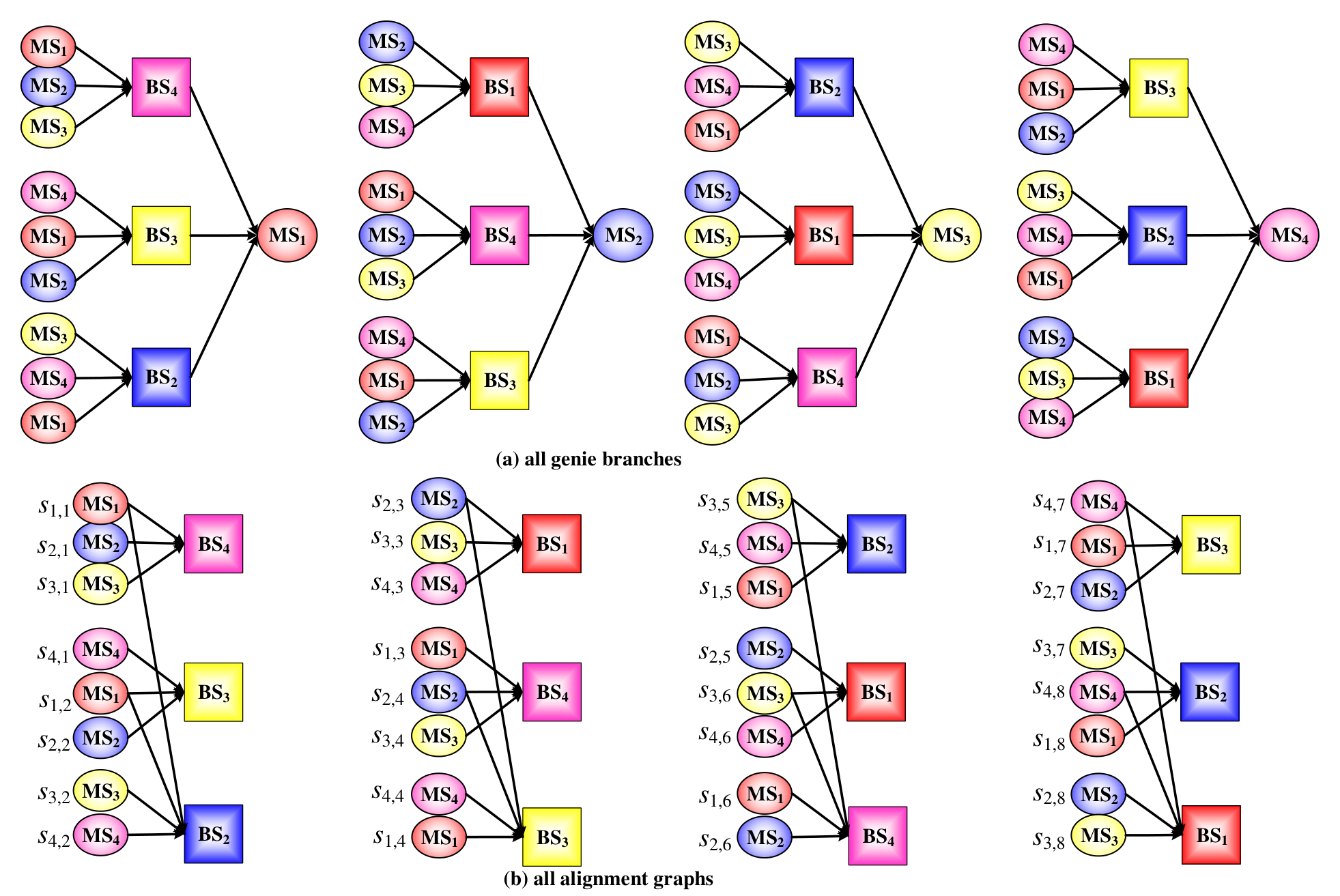
Refer to caption
Fig. 19: Genie branches and alignment graphs for Ex 4.

Following the similar analysis as Ex 11, we can obtain three alignment graphs shown in Fig. 18(b). According to these alignment graphs, we can obtain the alignment equations as follows,

{𝑯4,1​𝒖1,1+𝑯4,2​𝒖2,1+𝑯4,3​𝒖3,1=𝟎𝑯3,4​𝒖4,1+𝑯3,1​𝒖1,1+𝑯3,2​𝒖2,1=𝟎𝑯2,1​𝒖1,1+𝑯2,1​𝒖1,2+𝑯2,3​𝒖3,2+𝑯2,4​𝒖4,2=𝟎\displaystyle\left\{\begin{array}[]{l}\boldsymbol{H}_{4,1}\boldsymbol{u}_{1,1}+\boldsymbol{H}_{4,2}\boldsymbol{u}_{2,1}+\boldsymbol{H}_{4,3}\boldsymbol{u}_{3,1}=\boldsymbol{0}\\ \boldsymbol{H}_{3,4}\boldsymbol{u}_{4,1}+\boldsymbol{H}_{3,1}\boldsymbol{u}_{1,1}+\boldsymbol{H}_{3,2}\boldsymbol{u}_{2,1}=\boldsymbol{0}\\ \boldsymbol{H}_{2,1}\boldsymbol{u}_{1,1}+\boldsymbol{H}_{2,1}\boldsymbol{u}_{1,2}+\boldsymbol{H}_{2,3}\boldsymbol{u}_{3,2}+\boldsymbol{H}_{2,4}\boldsymbol{u}_{4,2}=\boldsymbol{0}\end{array}\right.
{𝑯1,2​𝒖2,3+𝑯1,3​𝒖3,3+𝑯1,4​𝒖3,3=𝟎𝑯4,1​𝒖1,3+𝑯4,2​𝒖2,4+𝑯4,3​𝒖3,4=𝟎𝑯3,2​𝒖2,3+𝑯3,2​𝒖3,3+𝑯3,4​𝒖4,4+𝑯3,1​𝒖1,4=𝟎\displaystyle\left\{\begin{array}[]{l}\boldsymbol{H}_{1,2}\boldsymbol{u}_{2,3}+\boldsymbol{H}_{1,3}\boldsymbol{u}_{3,3}+\boldsymbol{H}_{1,4}\boldsymbol{u}_{3,3}=\boldsymbol{0}\\ \boldsymbol{H}_{4,1}\boldsymbol{u}_{1,3}+\boldsymbol{H}_{4,2}\boldsymbol{u}_{2,4}+\boldsymbol{H}_{4,3}\boldsymbol{u}_{3,4}=\boldsymbol{0}\\ \boldsymbol{H}_{3,2}\boldsymbol{u}_{2,3}+\boldsymbol{H}_{3,2}\boldsymbol{u}_{3,3}+\boldsymbol{H}_{3,4}\boldsymbol{u}_{4,4}+\boldsymbol{H}_{3,1}\boldsymbol{u}_{1,4}=\boldsymbol{0}\end{array}\right.
{𝑯2,3​𝒖3,5+𝑯2,4​𝒖4,5+𝑯2,1​𝒖1,5=𝟎𝑯1,2​𝒖2,5+𝑯1,3​𝒖3,6+𝑯1,4​𝒖4,6=𝟎𝑯4,3​𝒖3,5+𝑯4,3​𝒖3,6+𝑯4,1​𝒖1,6+𝑯4,2​𝒖2,6=𝟎\displaystyle\left\{\begin{array}[]{l}\boldsymbol{H}_{2,3}\boldsymbol{u}_{3,5}+\boldsymbol{H}_{2,4}\boldsymbol{u}_{4,5}+\boldsymbol{H}_{2,1}\boldsymbol{u}_{1,5}=\boldsymbol{0}\\ \boldsymbol{H}_{1,2}\boldsymbol{u}_{2,5}+\boldsymbol{H}_{1,3}\boldsymbol{u}_{3,6}+\boldsymbol{H}_{1,4}\boldsymbol{u}_{4,6}=\boldsymbol{0}\\ \boldsymbol{H}_{4,3}\boldsymbol{u}_{3,5}+\boldsymbol{H}_{4,3}\boldsymbol{u}_{3,6}+\boldsymbol{H}_{4,1}\boldsymbol{u}_{1,6}+\boldsymbol{H}_{4,2}\boldsymbol{u}_{2,6}=\boldsymbol{0}\end{array}\right.
{𝑯3,4​𝒖4,7+𝑯3,1​𝒖1,7+𝑯3,2​𝒖2,7=𝟎𝑯2,3​𝒖3,7+𝑯2,4​𝒖4,8+𝑯2,1​𝒖1,8=𝟎𝑯1,4​𝒖4,7+𝑯1,4​𝒖4,8+𝑯1,2​𝒖2,8+𝑯1,3​𝒖3,8=𝟎\displaystyle\left\{\begin{array}[]{l}\boldsymbol{H}_{3,4}\boldsymbol{u}_{4,7}+\boldsymbol{H}_{3,1}\boldsymbol{u}_{1,7}+\boldsymbol{H}_{3,2}\boldsymbol{u}_{2,7}=\boldsymbol{0}\\ \boldsymbol{H}_{2,3}\boldsymbol{u}_{3,7}+\boldsymbol{H}_{2,4}\boldsymbol{u}_{4,8}+\boldsymbol{H}_{2,1}\boldsymbol{u}_{1,8}=\boldsymbol{0}\\ \boldsymbol{H}_{1,4}\boldsymbol{u}_{4,7}+\boldsymbol{H}_{1,4}\boldsymbol{u}_{4,8}+\boldsymbol{H}_{1,2}\boldsymbol{u}_{2,8}+\boldsymbol{H}_{1,3}\boldsymbol{u}_{3,8}=\boldsymbol{0}\end{array}\right.

which can be expressed as

𝑨ℓ𝑾Uℓ=𝟎,ℓ=1,2,3,4\displaystyle\boldsymbol{A}_{\ell}\boldsymbol{W}^{U}_{\ell}=\boldsymbol{0},~\ell=1,2,3,4

where

𝑨1\displaystyle\boldsymbol{A}_{1} =[𝑯4,1𝑯4,2𝑯4,3𝑯3,4𝑯3,1𝑯3,2𝑯2,1𝑯2,1𝑯2,3𝑯2,4]\displaystyle=\left[\begin{array}[]{llllllll}\boldsymbol{H}_{4,1}&\boldsymbol{H}_{4,2}&\boldsymbol{H}_{4,3}&&&&&\\ &&&\boldsymbol{H}_{3,4}&\boldsymbol{H}_{3,1}&\boldsymbol{H}_{3,2}&&\\ \boldsymbol{H}_{2,1}&&&&\boldsymbol{H}_{2,1}&&\boldsymbol{H}_{2,3}&\boldsymbol{H}_{2,4}\end{array}\right]
𝑨2\displaystyle\boldsymbol{A}_{2} =[𝑯1,2𝑯1,2𝑯1,4𝑯4,1𝑯4,2𝑯4,3𝑯3,2𝑯3,2𝑯3,4𝑯3,1]\displaystyle=\left[\begin{array}[]{llllllll}\boldsymbol{H}_{1,2}&\boldsymbol{H}_{1,2}&\boldsymbol{H}_{1,4}&&&&&\\ &&&\boldsymbol{H}_{4,1}&\boldsymbol{H}_{4,2}&\boldsymbol{H}_{4,3}&&\\ \boldsymbol{H}_{3,2}&&&&\boldsymbol{H}_{3,2}&&\boldsymbol{H}_{3,4}&\boldsymbol{H}_{3,1}\end{array}\right]
𝑨3\displaystyle\boldsymbol{A}_{3} =[𝑯2,3𝑯2,4𝑯2,1𝑯1,2𝑯1,3𝑯1,4𝑯4,3𝑯4,3𝑯4,1𝑯4,2]\displaystyle=\left[\begin{array}[]{llllllll}\boldsymbol{H}_{2,3}&\boldsymbol{H}_{2,4}&\boldsymbol{H}_{2,1}&&&&&\\ &&&\boldsymbol{H}_{1,2}&\boldsymbol{H}_{1,3}&\boldsymbol{H}_{1,4}&&\\ \boldsymbol{H}_{4,3}&&&&\boldsymbol{H}_{4,3}&&\boldsymbol{H}_{4,1}&\boldsymbol{H}_{4,2}\end{array}\right]
𝑨4\displaystyle\boldsymbol{A}_{4} =[𝑯3,4𝑯3,1𝑯3,2𝑯2,3𝑯2,4𝑯2,1𝑯1,4𝑯1,4𝑯1,2𝑯1,3]\displaystyle=\left[\begin{array}[]{llllllll}\boldsymbol{H}_{3,4}&\boldsymbol{H}_{3,1}&\boldsymbol{H}_{3,2}&&&&&\\ &&&\boldsymbol{H}_{2,3}&\boldsymbol{H}_{2,4}&\boldsymbol{H}_{2,1}&&\\ \boldsymbol{H}_{1,4}&&&&\boldsymbol{H}_{1,4}&&\boldsymbol{H}_{1,2}&\boldsymbol{H}_{1,3}\end{array}\right]
𝑾1U=[𝒖1,1T,𝒖2,1T,𝒖3,1T,𝒖4,1T,𝒖1,2T,𝒖2,2T,𝒖3,2T,𝒖4,2T]T\displaystyle\boldsymbol{W}^{U}_{1}=[\boldsymbol{u}_{1,1}^{T},\boldsymbol{u}_{2,1}^{T},\boldsymbol{u}_{3,1}^{T},\boldsymbol{u}_{4,1}^{T},\boldsymbol{u}_{1,2}^{T},\boldsymbol{u}_{2,2}^{T},\boldsymbol{u}_{3,2}^{T},\boldsymbol{u}_{4,2}^{T}]^{T}
𝑾2U=[𝒖2,3T,𝒖3,3T,𝒖4,3T,𝒖1,3T,𝒖2,4T,𝒖3,4T,𝒖4,4T​£​¬​𝒖1,4T]T\displaystyle\boldsymbol{W}^{U}_{2}=[\boldsymbol{u}_{2,3}^{T},\boldsymbol{u}_{3,3}^{T},\boldsymbol{u}_{4,3}^{T},\boldsymbol{u}_{1,3}^{T},\boldsymbol{u}_{2,4}^{T},\boldsymbol{u}_{3,4}^{T},\boldsymbol{u}_{4,4}^{T}\textsterling\textlnot\boldsymbol{u}_{1,4}^{T}]^{T}
𝑾3U=[𝒖3,5T,𝒖4,5T,𝒖1,5T,𝒖2,5T,𝒖3,6T,𝒖4,6T,𝒖1,6T,𝒖2,6T]T\displaystyle\boldsymbol{W}^{U}_{3}=[\boldsymbol{u}_{3,5}^{T},\boldsymbol{u}_{4,5}^{T},\boldsymbol{u}_{1,5}^{T},\boldsymbol{u}_{2,5}^{T},\boldsymbol{u}_{3,6}^{T},\boldsymbol{u}_{4,6}^{T},\boldsymbol{u}_{1,6}^{T},\boldsymbol{u}_{2,6}^{T}]^{T}
𝑾4U=[𝒖4,7T,𝒖1,7T,𝒖2,7T,𝒖3,7T,𝒖4,8T,𝒖1,8T,𝒖2,8T,𝒖3,8T]T\displaystyle\boldsymbol{W}^{U}_{4}=[\boldsymbol{u}_{4,7}^{T},\boldsymbol{u}_{1,7}^{T},\boldsymbol{u}_{2,7}^{T},\boldsymbol{u}_{3,7}^{T},\boldsymbol{u}_{4,8}^{T},\boldsymbol{u}_{1,8}^{T},\boldsymbol{u}_{2,8}^{T},\boldsymbol{u}_{3,8}^{T}]^{T}

For each BS, the number of received ICIs is (G−1)​K​d=24(G-1)Kd=24 ICIs. There are twelve alignment equations for four BSs. Therefore, the users can help each BS cancel three ICIs. Meanwhile, each BS can cancel the remaining M−K​d=29−8=21M-Kd=29-8=21 ICIs. As a result, all the ICIs can be jointly eliminated by the users and BSs, so that dQuan=8d^{\mathrm{Quan}}=8 is achievable by the designed IA transceiver.

From the examples, we can see that the genie branches can reflect how to align ICIs to make the transceivers to cancel the maximal number of ICIs. Therefore, the IA transceivers designed from the genie branches can achieve the DoF upper-bound for the networks with the antenna configurations in Region II.

VI Conclusion

In this paper, we provided the information theoretic maximal DoF for the GG-cell KK-user M×NM\times N symmetric MIMO-IBC network. For most antenna configurations in Region I, the information theoretic maximal DoF per user are M​N/(M+K​N)MN/(M+KN), which can be achieved by the asymptotic IA. The sum DoF linearly increase with GG but at the cost of infinite symbol extensions. For all antenna configurations in Region II, the information theoretic maximal DoF are the piecewise linear function of MM and NN, which can be achieved by the linear IA. The sum DoF are bounded by M+NM+N. To derive the DoF upper-bound for the networks with arbitrary antenna configurations, we proposed a unified way to construct the genie to help each BS or user resolve the maximal number of ICIs. By converting an information theoretic DoF upper-bound problem into a linear algebra problem, we obtained the closed-form DoF upper-bound expression for general case. The constructed genies constituted a genie tree, which indicates how to introduce genies to derive the tightest DoF upper-bound and how to align ICIs to derive the maximal achievable DoF. From the genie tree, we designed a non-iterative linear IA transceiver, which can achieve the information theoretic maximal DoF in Region II. The basic principles to derive the DoF upper-bound and design the feasible IA transceiver can be extended into more general asymmetric networks.

References

  • [1] C. Wang, T. Gou, and S. A. Jafar, “Subspace alignment chains and the degrees of freedom of the three-user MIMO Interference Channel,” IEEE Trans. Inf. Theory, vol. 60, no. 5, 2432–2479, May 2014.
  • [2] S. A. Jafar and M. J. Fakhereddin, “Degrees of freedom for the MIMO interference channel,” IEEE Trans. Inf. Theory, vol. 53, no. 7, pp. 2637–2642, Jul. 2007.
  • [3] V. R. Cadambe and S. A. Jafar, “Interference alignment and degrees of freedom of the KK-user interference channel,” IEEE Trans. Inf. Theory, vol. 54, no. 8, pp. 3425–3441, Aug. 2008.
  • [4] G. Bresler, D. Cartwright, and D. Tse, “Geometry of the 3-user MIMO interference channel,” in Proc. Allerton, Sep. 2011.
  • [5] T. Gou and S. A. Jafar, “Degrees of freedom of the KK user M×NM\times N MIMO interference channel,” IEEE Trans. Inf. Theory, vol. 56, no. 12, pp. 6040–6057, Dec. 2010.
  • [6] A. Ghasemi, A. Motahari, A. Khandani, “Interference Alignment for the KK User MIMO Interference Channel,” in Proc. IEEE ISIT, Jun. 2010.
  • [7] C. M. Yetis, T. Gou, and S. A. Jafar, Genie chains: Exploring Outer Bounds on the degrees of freedom of MIMO Interference Networks, arXiv:1404.2258v1 [cs.IT], Apr. 2014.
  • [8] L. Ruan, V. K. N. Lau, M. Z. Win, “The feasibility conditions for interference alignment in MIMO networks,” IEEE Trans. Signal Process., vol. 61, no. 8, pp. 2066¨C2077, Apr. 2013.
  • [9] O. Gonzalez, C. Beltran, I. Santamaria, “A feasibility test for linear interference alignment in MIMO channels with constant coefficients,” IEEE Trans. Inf. Theory, vol. 60, n. 3, pp. 1840-1856, March 2014.
  • [10] G. Sridharan and Wei Yu, “Degrees of Freedom of MIMO Cellular Networks: Decomposition and Linear Beamforming Design,” IEEE Trans. Inf. Theory, vol. 61, no. 6, pp. 3339-3364, 2015.
  • [11] J. Sun, Y. Liu, and G. Zhu, “On the degrees of freedom of the cellular network,” in Proc. IEEE ICC, May 2010.
  • [12] S. Park and I. Lee, “Degrees of freedom of multiple broadcast channels in the presence of inter-cell interference,” IEEE Trans. Commun., vol. 59, no. 5, pp. 1481-1487, May 2011.
  • [13] T. Kim, D. J. Love, B. Clerckx, and D. Hwang, “Spatial degrees of freedom of the multicell MIMO multiple access channel,” in Proc. IEEE GLOBECOM, Dec. 2011.
  • [14] C. M. Yetis, T. Gou, S. A. Jafar, and A. H. Kayran, “On feasibility of interference alignment in MIMO interference networks,” IEEE Trans. Signal Process., vol. 58, no. 9, pp. 4771–4782, Sep. 2010.
  • [15] K. Gomadam, V. R. Cadambe, and S. A. Jafar, “Approaching the capacity of wireless networks through distributed interference alignment,” in Proc. IEEE GLOBECOM, Dec. 2008.
  • [16] G. Bresler, D. Cartwright, and D. Tse, “Feasibility of interference alignment for the MIMO interference channel,” IEEE Trans. Inf. Theory, vol. 60, no. 9, pp. 5573–5586, Sep. 2014.
  • [17] M. Razaviyayn, L. Gennady, and Z. Luo, “On the degrees of freedom achievable through interference alignment in a MIMO interference channel,” IEEE Trans. Signal Process., vol. 60, no. 2, pp. 812-821, Sep. 2012.
  • [18] B. Zhuang, R. A. Berry, and M. L. Honig, “Interference alignment in MIMO cellular networks,” in Proc. IEEE ICASSP, May 2011.
  • [19] T. Liu and C. Yang, “On the feasibility of interference alignment for MIMO interference broadcast channels with constant coefficients,” IEEE Trans. Signal Process., vol. 61, no. 9, pp. 2178-2191, May 2013.
  • [20] T. Cover and J. Thomas, Elements of Information Theory, Wiley, 2006.
  • [21] W. B. Jones and W. J. Thron, Continued Fractions: Analytic Theory and Applications, Addison-Wesley, Reading, Mass, 1980.
  • [22] J. A. Bondy and U.S.R. Murty, Graph theory with applications, London: Macmillan, 1976.
  • [23] D. Meyer, Matrix analysis and applied linear algebra, Society for Industrial and Applied Mathematics (SIAM), 2000.
[Uncaptioned image] Tingting Liu (S’09–M’11) received the B.S. and Ph.D. degrees in signal and information processing from Beihang University, Beijing, China, in 2004 and 2011, respectively. From December 2008 to January 2010, she was a visiting student with the School of Electronics and Computer Science, University of Southampton, Southampton, U.K. She is currently an associate professor in the School of Electronics and Information Engineering, Beihang University (BUAA). Her PhD thesis was received ¡°2013 National Excellent Doctoral Thesis Nomination¡±and ¡°2012 Excellent Beijing Doctoral Thesis Award¡±. Her research interests include wireless communications and signal processing, the interference management for ultra-dense networks.
[Uncaptioned image] Chenyang Yang (SM’08) received the M.S.E and Ph.D. degrees in electrical engineering from Beihang University (formerly Beijing University of Aeronautics and Astronautics), Beijing, China, in 1989 and 1997, respectively. Since 1999, she has been a Full Professor with the School of Electronic and Information Engineering, Beihang University. She has published more than 200 international journal and conference papers and filed more than 60 patents in the fields of energy-efficient transmission, coordinated multi-point, interference management, cognitive radio, relay, etc. Her recent research interests include green radio, local caching, and other emerging techniques for next generation wireless networks. Prof. Yang was the Chair of the Beijing chapter of the IEEE Communications Society during 2008-2012 and the Membership Development Committee Chair of the Asia Pacific Board, IEEE Communications Society, during 2011- 2013. She has served as a Technical Program Committee Member for numerous IEEE conferences and was the Publication Chair of the IEEE International Conference on Communications in China 2012 and a Special Session Chair of the IEEE China Summit and International Conference on Signal and Information Processing (ChinaSIP) in 2013. She served as an Associate Editor for the IEEE TRANSACTIONS ON WIRELESS COMMUNICATIONS during 2009-2014 and a Guest Editor for the IEEE JOURNAL ON SELECTED TOPICS IN SIGNAL PROCESSING published in February 2015. She is currently an Associate Editor-in-Chief of the Chinese Journal of Communications and the Chinese Journal of Signal Processing. She was nominated as an Outstanding Young Professor of Beijing in 1995 and was supported by the First Teaching and Research Award Program for Outstanding Young Teachers of Higher Education Institutions by the Ministry of Education during 1999-2004.