A new transfer-matrix algorithm for exact enumerations: self-avoiding walks on the square lattice
Abstract
We recently published [J. Phys A: Math. Theor. 45 115202 (2012)] a new and more efficient implementation of a transfer-matrix algorithm for exact enumerations of self-avoiding polygons. Here we extend this work to the enumeration of self-avoiding walks on the square lattice. A detailed comparison with our previous best algorithm shows very significant improvement in the running time of the new algorithm. The new algorithm is used to extend the enumeration of self-avoiding walks to length 79 from the previous record of 71 and for metric properties, such as the average end-to-end distance, from 59 to 71.
1 Introduction
Self-avoiding walks (SAW) on regular lattices is one of the most important and classic combinatorial problems in statistical mechanics [1]. SAW are often considered in the context of lattice models of polymers [2, 3]. The fundamental problem is the calculation (up to translation) of the number of SAW, , with steps. As most interesting combinatorial problems, SAW have exponential growth, , where is the connective constant, is a (known) critical exponent [4, 5], and is a critical amplitude. Furthermore the enumeration of SAW have traditionally served as a benchmark for both computer performance and algorithm design. A -step self-avoiding walk on a regular lattice is a sequence of distinct vertices such that each vertex is a nearest neighbour of it predecessor. SAW are considered distinct up to translations of the starting point . We shall use the symbol to mean the set of all SAW of length . If and are nearest neighbours we can form self-avoiding polygons (SAP) by inserting an edge between the end-points.

The enumeration of SAW and SAP has a long and glorious history, which for the square lattice has recently been reviewed in [6]. Suffice to say that early calculations were based on various direct counting algorithms of exponential complexity, with computing time growing asymptotically as , where , the connective constant for SAW. Enting [7] was the first to produce a major breakthrough by applying transfer matrix (TM) methods to the enumeration of SAP on finite lattices. Results for finite lattices (rectangles in the case of the square lattice) are then combined to obtain a series expansion for the infinite lattice. This so called finite lattice method (FLM) led to a very significant reduction in complexity to , so . More recently we [8] refined the algorithm using the method of pruning and reduced the complexity to . Pruning is quite simple in theory and essentially works by calculating the minimal order at which a configuration created by the transfer matrix algorithm would contribute to the generations function; if this order exceeds a pre-set maximal order we discard (prune) the configuration. The extension of the FLM to SAW enumeration had to wait until 1993 when Conway, Enting and Guttmann [9] implemented an algorithm with complexity . In 2004 we [10] implemented a TM algorithm based on the same ideas of pruning used to improve the SAP algorithm. It appears that this pruning algorithm has a computational complexity of very close to the CEG algorithm.
All of the above TM algorithms are based on keeping track of the way partially constructed SAW are connected to the left of a cut-line bi-secting the given finite lattice (rectangles in the case of the square lattice). Recently Clisby and Jensen [11] devised a new and more efficient implementation of the transfer-matrix algorithm for SAP. In that implementation we took a new approach and instead kept track of how a partially constructed SAP must be connected to the right of the cut-line. In this paper we extend this approach to the enumeration of SAW. The major gain is that is now quite simple to calculate the order at which a transfer-matrix configuration will contribute, and this in turn results in a much faster algorithm. The draw-back is that some updating rules become much more complicated.
2 The finite-lattice method and TM algorithms
All TM algorithms used to enumerate SAW on the square lattice build on the pioneering work of Enting [7] who enumerated square lattice self-avoiding polygons using the finite lattice method. The first terms in the series for the SAW generating function can be calculated using transfer matrix techniques to count the number of walks in rectangles unit cells wide and cells long. Due to the symmetry of the square lattice one need only consider rectangles with . Any walk spanning such a rectangle has a length of at least steps. By adding the contributions from all rectangles of width (where the choice of depends on available computational resources) and length (with contributions from rectangles with counted twice) the number of walks per vertex of an infinite lattice is obtained correctly up to length .
2.1 Outline of the new TM algorithm
The basic idea of the new algorithm can best be illustrated by considering the specific example of a SAW given in figure 1. Clearly any SAW is topologically equivalent to a line and therefore has exactly two end-points. If we cut the SAW by a vertical line as shown in figure 2 (the dashed lines) we see that the SAW is broken into several pieces to the left and right of the cut-line. On either side of the cut-line we have a set of arcs connecting two edges on the cut-line and at most two line pieces connected to the end-points of the SAW. This means that at any stage a given configuration of occupied edges along the cut-line can be described in two ways. We can describe how the edges are connected forming either arcs or line pieces to the left or right of the cut-line. As we move the cut-line from left to right we can keep track of what happened in the past, that is how the pieces are connected to the left, or prescribe what must happen in the future, that is how edges are to be connected to the right of the cut-line so as to form a valid SAW. The ‘traditional’ TM algorithm keeps track of the past connections. In the new algorithm we keep track of future connections. There is a natural bijection between the configurations which are generated by the two approaches due to the left-right symmetry of the finite lattice. The improved performance of the new approach comes purely from the enhanced efficiency of the pruning algorithm.

An edge of an arc on the cut-linei is assigned one of two labels depending on whether it is the lower or upper end of an arc. In addition there are at most two free edges which are not connected to any occupied edge on the cut-line. Any configuration along the cut-line can thus be represented by a set of edge states , where
| (1) |
If we read from the bottom to the top, the configuration or signature along the cut-lines of the SAW in figure 2 are, respectively, , , and . Since crossings are not permitted this encoding uniquely describes how the occupied edges are connected. As the cut-line is moved a free edge may become connected to a new occupied edge thus forming an arc or an existing arc may form connections to new edges leading to a ‘re-configuration’ of the arcs.

In applying the transfer matrix technique to the enumeration of SAW we regard them as sets of edges on the finite lattice with the properties:
- (1)
A weight is associated with each occupied edge.
- (2)
All vertices (except the two end-points) are of degree 0 or 2.
- (3)
Apart from isolated sites, the graph has a single connected component.
- (4)
Each graph must span the rectangle from left to right and from bottom to top.
The most efficient implementation of the TM algorithm generally involves moving the cut-line in such a way as to build up the lattice vertex by vertex as illustrated in figure 3.
Constraint (1) is trivial to satisfy. The sum over all contributing graphs (valid SAW) is calculated as the cut-line is moved through the lattice. For each configuration of occupied or empty edges along the intersection we maintain a generating function for partial walks with signature . In exact enumeration studies is a truncated polynomial , where is conjugate to the number of occupied edges. In a TM update each source signature (before the cut-line is moved) gives rise to new target signatures (after the move of the cut-line) and or 2 new occupied edges are inserted leading to the update .
Constraint (2) is easy to satisfy. If both kink edges are empty we can leave both new edges empty, insert a new arc by occupying both of the new edges or we may insert a single new edge. If one of the kink edges is occupied then one or none of the new edges will be occupied. If both of the kink edges are occupied both of the new edges must be empty. It is easy to see that these rules leads to graphs satisfying constraint (2). The specific updating rules will naturally depend on the state of the incoming edges as we shall explain in some detail below.
In order to satisfy constraint (4) we need to add more information to a signature. In addition to the usual labeling of the edges intersected by the cut-line we also have to indicate whether the partially completed SAW has reached neither, both, the lower, or the upper borders of the rectangle. We therefore add two extra ‘virtual’ edge states and to the signature. Here ( ) is 0 or 1 if the bottom (top) of the rectangle has or has not been touched.
We shall now give some details of the updating rules which results in the enumeration of all SAW. Constraint (3) will be satisfied by these rules. Firstly we look at the construction of the first column of a finite rectangle. To start a SAW at a vertex on the left border of the rectangle we insert either an arc or a single occupied edge into the totally empty configuration. If we insert an arc both occupied edges must be free; this is so because there are no other occupied edges along the cut-line and the two edges can’t be connected since this would result in a polygon. If we insert a single occupied edge it must be free. Note that it is only during the build-up of the first column that this initial insertion into the completely empty state occurs and this is the only time that new free edges can be created. These rules also ensure that all SAW touch the left-most border of the rectangle.
The updating rules depends primarily on the states of the two incoming edges in the kink; secondarily on the state of the edge immediately below the kink; and finally edge states further from the kink may be affected by the insertion of new occupied edges. The simplest case is that in which both incoming edges are occupied. Recall that the encoding in the new algorithm prescribes how occupied edges are to be connected. We can thus join two edges at the kink only if they belong to the same arc. Hence the only valid case is the kink-state ‘12’. Two situations arise when arc edges are joined at the kink; either there are other occupied edges along the cut-line and we just proceed with the calculation leaving the outgoing edges empty; or all other edges are empty and a completed SAW is formed and added to the running total for the SAW generating function (provided that the SAW has touched both the bottom and top border of the rectangle). All other kink states with two occupied edges (‘11’, ‘22’, ‘21’, ‘13’, ‘23’, ‘31’, ‘32’, ‘33’) are forbidden since they would correspond to connecting occupied edges which should not have been connected. Avoiding these situations is part of the updating rules for the cases where there is one or two empty edges in the kink state. Another consequence of this strong restriction on possible kink states is that we may arrange things such that the vertical kink-edge is empty unless part of the ‘12’ state. In other words the only possible kink-states are ‘00’, ‘10’, ‘20’, ‘30’ and ‘12’.
If the incoming kink state is ‘10’ this edge must be continued along one of the two outgoing edges. The vertical edge can only be occupied if the edge immediately below the kink is empty (otherwise a forbidden kink-state with two occupied edges would be formed). When the incoming kink state is ‘20’ we continue the walk along one of the two outgoing edges. The vertical edge can only be occupied if the edge immediately below the kink is ‘empty’ or ‘lower’. In the latter case we check if there are other occupied edges in the signature; if not we have a completed SAW. When the incoming kink state is ‘30’ we may continue the walk along one of the two outgoing edges as for the ‘10’ case or we can terminate the edge at this vertex creating a new end-point for the walk. In the latter case we again check if there are other occupied edges in the signature and if not we add the generating function to the running total as per the ‘20’ case.
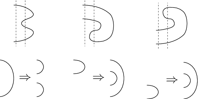
Finally we turn to the case where the incoming edges are empty. This case is by far the most complicated. Obviously we can leave the outgoing edges empty. If the signature has no free edges the only other possibility is to add a new arc on the outgoing edges and connect the new arc to an existing arc somewhere else on the cut-line. This update is the same as for the SAP algorithm and was described in [11]. For completeness we briefly outline the updating rules for this case. The two new occupied edges must connect to existing connected edges provided these are accessible (more on this later). In figure 4 we show the two basic situations: The new occupied edges are either placed inside an existing arc or they are placed outside the arc. In the first case, shown to the left in figure 4, the upper (lower) end of the inserted arc must connect with the upper (lower) end of the existing arc, in terms of the edges involved the states change from ‘1002’ to ‘1212’ (reading from bottom to top). In the second case, in the middle of the figure, the upper (lower) end of the inserted arc must connect with the lower (upper) end of the existing arc, in terms of the edges involved the states change from ‘0012’ to ‘1122’. So both new occupied edges become ‘lower’ arc-ends while the existing lower arc-end is changed to an upper arc-end. Shown to the right in figure 4, there is also a symmetric case where the new arc is placed above the existing arc leading to the state change ‘1200’ to ‘1122’.
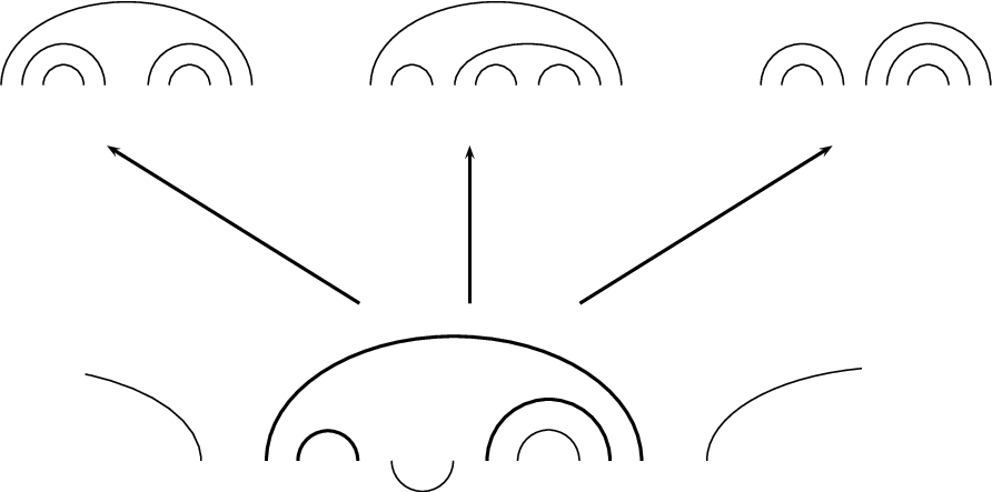
The newly inserted arc can connect to any existing arc that can be reached without crossing another arc. The general situation is illustrated in figure 5 where we see that the new arc can be connected to three existing arcs (indicated by thick lines). The second arc to the right of the new arc is nested inside an existing arc and can therefore not be reached without crossing the enclosing arc. Likewise any arcs outside the large arc enclosing the new arc are inaccessible. So in this case the insertion of a single new arc gives rise to three new arc configurations as illustrated in the top panels of figure 5. The states of the edges in the new arc configurations are obtained by applying the appropriate basic arc insertion from above.
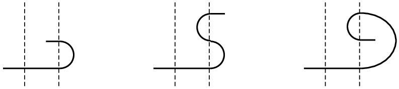
Next we turn to the case where there is one or two free edges in the source signature. In figure 6 we show schematically how a configuration involving a single free edge may change as we insert a new occupied edge or a new arc; in the latter case the free edge may connect to either the lower or upper edge of the new arc. If there are other arcs in the existing configuration these will be unaffected by the insertion. The insertions shown in the figure are possible provided the free edge is accessible, i.e., not hidden inside an existing arc. If two free edges were present and accessible we could connect the newly inserted edge(s) to either of the two free edges and the basic update would be the same.
Since we use the form of the TM algorithm where we ‘grow’ the lattice a single vertex at a time we must split the updating rule into four cases depending on the state of the edge immediately below the kink.
-
Free: We can insert an arc on the two outgoing edges. The lower edge of the arc connects to the existing free edge. The local kink configuration ’300’ becomes ‘123’. We can also insert an edge along one of the outgoing edges. If we occupy the vertical edge this connects with the free edge below. If no other occupied edges are present a completed SAW is formed; otherwise we change the local configuration ‘300’ to ‘120’. Finally we may insert a single occupied edge along the horizontal outgoing edge. This edge must be connected to an existing free edge. So we search above (below) the kink for an accessible free edge and if we find one the state of the outgoing occupied edge is ‘lower’ (‘upper’) while the state of the existing free edge is changed to ‘upper’ (‘lower’). Note that the insertion of a single occupied edge reduces the number of free edges by one.
-
Upper/Lower: We can insert an occupied edge on the horizontal outgoing edge provided there is an accessible free edge above or below the kink.
-
Empty: In this case we can occupy the horizontal or vertical outgoing edge with a single edge or occupy both outgoing edges with an arc; in all cases this only happens if there is an accessible free edge above or below the kink. In the case where we connect to a free end above the kink the change in the signature is schematically that the existing signature becomes , , and , respectively, as illustrated in figure 6.
At this stage it seems nothing has been gained. Some updates simplify while edge- or arc-insertion becomes much more complicated. The pay-off comes when we look to pruning.
2.2 Pruning
The principle behind pruning is quite simple and briefly works as follows. Firstly, for each signature we keep track of the current minimum number of occupied edges already inserted to the left of the cut-line in order to build up that particular configuration. Secondly, we calculate the minimum number of additional steps required to produce a valid walk. There are three contributions, namely the number of steps required to connect all occupied edges into a single walk, the number of steps needed (if any) to ensure that the walk touches both the lower and upper border, and finally the number of steps needed (if any) to extend at least edges in the length-wise direction (remember we only need rectangles with ). If the sum we can discard the partial generating function for that configuration, and of course the configuration itself, because it will not make a contribution to the SAW count up to the maximal length we are trying to obtain. For instance SAW spanning a rectangle with a width close to have to be almost staircase like lines, so that very convoluted walks aren’t possible on these types of rectangles.
In the original approach pruning can be very complicated. With deeply nested configurations one simply has to search through all possible ways of connecting existing occupied edges in order to find the connection pattern, which minimises the number of additional steps required to form a valid SAW. In the new approach almost all of the complications of pruning are gone. Since connections between edges are already prescribed there is one and only one way of completing the SAW! The only complicating factor is that in order to calculate we need to know the nesting level of each arc. The number of edges it takes to connect the two edges of an arc at positions and is simply . Note that only arcs contribute to the step count required to connect the occupied edges in order to form a SAW. Free edges only enter into consideration when we have to calculate the number of steps required to connect the SAW to the lower and upper borders of the rectangle and ensure that the SAW extends at least edges in the length-wise direction. This pruning procedure can be performed in operations.
2.3 Comparative study of the algorithms
In analysing the complexity of the two algorithms, we note that the update step when the cut-line is moved may result in signatures for the previous algorithm, and for the new one. However, in the average case we still expect the new algorithm to create signatures, as connections with distant occupied edges typically do not contribute to the generating function (either because the edges are inaccessible, or the resulting partial SAW configurations have too many occupied edges and are pruned away). For pruning, we believe that the complexity of the old algorithm is exponential in , whereas for the new algorithm the complexity is .
In table 1 we compare the resources used by the two algorithms in a calculation of the number of SAW of length up to . From this it is clear that the new approach is much more efficient with substantial savings in time. The required number of configurations and terms go down very slightly while the total CPU time decreases by about 70% for . In figure 7 we plot the ratio of the time used by the two algorithms versus and we notice a clear (reasonably monotonic) decrease with . The slight scatter in the data can have many causes one being that the calculations were done on multi-core processors which can be sensitive to what else is being computed on the processor.
| Old Algorithm | New Algorithm | |||||
|---|---|---|---|---|---|---|
| Configs | Terms | Time | Configs | Terms | Time | |
| 41 | 258167 | 949978 | 00:04:03 | 237959 | 237959 | 00:02:07 |
| 43 | 458272 | 1656198 | 00:09:10 | 417066 | 1514488 | 00:04:27 |
| 45 | 794580 | 2922585 | 00:20:33 | 728771 | 2669337 | 00:09:31 |
| 47 | 1404805 | 5204306 | 00:45:03 | 1293429 | 4646527 | 00:20:49 |
| 49 | 2479142 | 9155623 | 01:33:09 | 2257207 | 8153021 | 00:38:11 |
| 51 | 4303075 | 16201349 | 03:15:17 | 3932460 | 14608709 | 01:20:35 |
| 53 | 7698939 | 28342605 | 06:55:35 | 6945579 | 25443108 | 02:33:12 |
| 55 | 13457105 | 49905607 | 15:21:27 | 12198903 | 44768207 | 05:24:34 |
| 57 | 23486864 | 89241921 | 32:22:55 | 21475037 | 78816673 | 11:08:06 |
| 59 | 42037696 | 154839352 | 67:15:57 | 37409087 | 138688285 | 21:41:24 |
| 61 | 72844262 | 275510888 | 138:10:11 | 65787437 | 245737647 | 39:58:11 |

3 Extended SAW enumerations
The transfer-matrix algorithm is eminently suited to parallel computations and here we used the approach described in [12, 10] to extend the enumeration of SAW from length 71 [10] to 79. In addition we have extended the series for some metric properties (such as the end-to-end distance) from 59 to 71 step SAW. One of the main ways of achieving a good parallel algorithm using data decomposition is to try to find an invariant under the operation of the updating rules. That is we seek to find some property of the configurations along the cut-line which does not alter in a single iteration. The algorithm for the enumeration of SAW is quite complicated since not all possible configurations occur due to pruning, and the insertion of new occupied edges can change the state of an occupied edge far removed. However, there still is an invariant since any edge not directly involved in the update cannot change from being empty to being occupied and vice versa. That is only the kink edges can change their occupation status. This invariant allows us to parallelise the algorithm in such a way that we can do the calculation completely independently on each processor with just two redistributions of the data set each time an extra column is added to the lattice.
The bulk of the calculations for this paper were performed on the cluster of the NCI National Facility at ANU. The NCI peak facility was a Sun Constellation Cluster with 1492 nodes in Sun X6275 blades, each containing two quad-core 2.93GHz Intel Nehalem CPUs with most nodes having 3GB of memory per core (24GB per node). It took a total of about 16500 CPU hours to enumerate SAW up to length 79. We used up to 400 processors (or more accurately cores) and up to 1TB of memory. Some details of resource use are given below.
The integer coefficients occurring in the series expansion become very large and the calculation was therefore performed using modular arithmetic and the series was calculated modulo various integers and then reconstructed at the end using the Chinese remainder theorem. In the calculation of we used the moduli and which allowed us to represent correctly. The NCI cluster is a heavily used shared computing facility so our major constraint was CPU time rather than memory. For this reason we chose to perform the calculation for all in the same run. Effectively this increased the memory requirement by some 50% but only results in an increase in running time of some 15% (compared to a run using a single ).
The algorithm for the calculation of metric properties was described in [10] and we won’t repeat it here. Suffice to say that the algorithm requires the multiplication of integers so to avoid overflow we have to use moduli smaller than (signed integers) and in practise we use the largest prime numbers smaller than . In this case we had to use 4 primes to represent the integer coefficients and again we calculate series modulo all 4 primes in a single run. The calculation of the metric properties took a total of about 8000 CPU hours.
Table 2 lists the new terms obtained in this work for the number of SAW with perimeter 72–79. The full series are available at www.ms.unimelb.edu.au/˜iwan.
| 72 | 11107224538074654820152678182884 |
| 73 | 29442884996760677051402398150644 |
| 74 | 78023796077779727644807609460228 |
| 75 | 206797849568186990141402577046860 |
| 76 | 547952781764285893561169365957068 |
| 77 | 1452142167241575828091155500636684 |
| 78 | 3847327231644550282490410907667972 |
| 79 | 10194710293557466193787900071923676 |
3.1 Resource use
| Procs | Time | Min Conf | Max Conf | Min Term | Max Term | -min | -max | |
|---|---|---|---|---|---|---|---|---|
| 20 | 48 | 71 | 13148840 | 13269033 | 105620097 | 110799361 | 810 | 839 |
| 21 | 64 | 130 | 17692356 | 17973627 | 123093203 | 128413924 | 1012 | 1047 |
| 22 | 96 | 233 | 19262398 | 19818552 | 117757527 | 124452609 | 1212 | 1269 |
| 23 | 128 | 366 | 20979889 | 21455635 | 117135449 | 123820823 | 1303 | 1375 |
| 24 | 192 | 548 | 18927269 | 19259207 | 101433367 | 105334639 | 1361 | 1427 |
| 25 | 256 | 766 | 18383861 | 18745970 | 97671731 | 100083799 | 1457 | 1530 |
| 26 | 256 | 1044 | 23823377 | 24298689 | 117585078 | 121505762 | 1692 | 1768 |
| 27 | 400 | 1320 | 18909565 | 19281974 | 86963922 | 90679689 | 1697 | 1792 |
| 28 | 400 | 1603 | 22401386 | 22874296 | 95884039 | 98305119 | 1779 | 1876 |
| 29 | 400 | 1837 | 25481090 | 25840551 | 100310512 | 102930835 | 1814 | 1919 |
| 30 | 400 | 2011 | 26643740 | 27211923 | 95761871 | 98905129 | 1843 | 1949 |
| 31 | 400 | 2134 | 26570470 | 26955370 | 86419643 | 88567259 | 1797 | 2078 |
| 32 | 400 | 1997 | 23597167 | 23964367 | 65382639 | 67106763 | 1679 | 1800 |
| 33 | 400 | 1367 | 17534151 | 18395643 | 46251198 | 51913381 | 1341 | 1426 |
| 34 | 280 | 685 | 17266488 | 17639105 | 38259003 | 39771128 | 932 | 1047 |
| 35 | 128 | 231 | 13357320 | 23294968 | 24188367 | 45450559 | 480 | 1357 |
In table 3 we have listed the main resources used by the parallel algorithm in order to enumerate SAW up to length 79. For each width we first list the number of processors used and the total CPU time in hours required to complete the calculation for a given width. One of the main issues in parallel computing is that of load balancing. That is, we wish to ensure to the greatest extent possible that the workload is shared equally among all the processors. This aspect is examined via the numbers in columns 4–9. At any given time during the calculation each processor handles a subset of the total number of configurations. For each processor we monitor the maximal number of configurations and terms retained in the generating functions. Note that the number of terms listed is per modulo ; so in total three times this number is actually stored. The load balancing can be roughly gauged by looking at the largest (Max Conf) and smallest (Min Conf) maximal number of configurations handled by individual processors during the execution of the program. In columns 6 and 7 are listed the largest (Max Term) and smallest (Min Term) maximal number of terms retained in the generating functions associated with the subset of configurations. As can be seen the algorithm is very well balanced. Finally in columns 8 and 9 we have listed the minimal and maximal total time (in seconds) spent by any processor in the redistribution part of the algorithm and as can be seen this part of the algorithm takes a total of some 15% of the CPU time. Note that most of this time is spent preparing for the redistribution and processing the data after it has been moved. The actual time spent in the MPI message passing routines is less than 5% of total CPU time.
4 Series analysis and results
The number of SAW of length , believed to have the asymptotic behaviour
| (2) |
where is the connective constant and is a critical exponent. We shall also study the associated generating function
| (3) |
so the generating function has a singularity at . As for the three metric properties we have for the mean-square end-to-end distance of step SAW that
| (4) |
where is a new critical exponent, with associated generating function
| (5) |
The mean-square radius of gyration of step SAW is defined as
| (6) |
and has an associated generating function
| (7) |
where the factors under the sum ensure that the coefficients are integer valued. Finally, the mean-square distance of a monomer from the end-points of step SAW is
| (8) |
with generating function
| (9) |
The critical exponents are believed to be universal in that they only depend on the dimension of the underlying lattice. on the other hand is non-universal. For SAW in two dimensions the critical exponents and have been predicted exactly, though non-rigorously, using Coulomb-gas arguments [4, 5].
The asymptotic form (2) for only explicitly gives the leading contribution. In general one would expect corrections to scaling so
| (10) |
In addition to “analytic” corrections to scaling of the form , there are “non-analytic” corrections to scaling of the form , where the correction-to-scaling exponent isn’t an integer. In fact one would expect a whole sequence of correction-to-scaling exponents , which are both universal and also independent of the observable. Much effort has been devoted to determining the leading non-analytic correction-to-scaling exponent for two-dimensional SAW. In [13] we studied the amplitudes and the correction-to-scaling exponents for two-dimensional SAW, using a combination of series-extrapolation and Monte Carlo methods. We enumerated all self-avoiding walks up to 59 steps on the square lattice, and up to 40 steps on the triangular lattice, measuring the metric properties mentioned above, and then carried out a detailed and careful analysis of the data in order to accurately estimate the amplitudes and correction-to-scaling exponent. This analysis unequivocally confirmed that the data is consistent with the exact value as obtained from Coulomb-gas arguments [4, 5].
Besides the physical singularity there is another singularity at [14, 15] which has a critical exponent consistent with the exact value . Given the value for the non-analytic correction-to-scaling exponent the asymptotic form used in [13] was
| (11) | |||||
There will also be sequences of additional terms arising from higher-order correction-to-scaling exponents.
To test the singularity structure of the generating functions we used the numerical method of differential approximants [16]. We will not describe the method here and refer the interested reader to [16] for details; and Chapter 8 of [17] for an overview of our use of the method. In table 4 we list estimates for the critical point and exponent . The estimates were obtained by averaging values obtained from second and third order differential approximants. For each order of the inhomogeneous polynomial we averaged over those approximants to the series which used at least the first 71 terms of the series. The quoted error for these estimates reflects the spread (basically one standard deviation) among the approximants. Note that these error bounds should not be viewed as a measure of the true error as they cannot include possible systematic sources of error. Based on these estimates we conclude that and . The estimate for is consistent with though several orders of magnitude less accurate than the estimate obtained from an analysis of the SAP series [11]; and due to our conservative error-bars the estimate for is just consistent with the exact value .
| Second order DA | Third order DA | |||
|---|---|---|---|---|
| 0 | 0.37905227478(90) | 1.3437488(14) | 0.37905227604(95) | 1.3437435(27) |
| 2 | 0.37905227492(70) | 1.3437391(34) | 0.37905227663(33) | 1.3437452(14) |
| 4 | 0.37905227679(32) | 1.3437440(12) | 0.37905227658(38) | 1.3437456(16) |
| 6 | 0.379052276419(97) | 1.34374286(30) | 0.37905227672(32) | 1.3437457(12) |
| 8 | 0.37905227617(35) | 1.34374299(63) | 0.37905227670(22) | 1.34374578(84) |
| 10 | 0.37905227630(17) | 1.34374334(46) | 0.37905227670(28) | 1.34374564(88) |
To gauge whether or not the estimates truly are as well converged as the results in table 4 would suggest we find it useful to plot the actual individual estimates against (where is the last terms used to form a given differential approximant). In the left panel of figure 8 we have plotted the estimates for as a function of . Each point represents an estimate from a third order differential approximant. The approximants appear very well converged and given the very high resolution of the abscissa there is no sign of any significant systematic drift. In the right panel we plotted the estimate for versus the corresponding estimates for . If the conjecture for the exact value of is correct these estimates should ideally pass through the point of intersection between the conjectured value and the extremely accurate estimate for obtained from the SAP series. All in all these plots clearly are consistent with the exact value .

4.1 Amplitudes
In our paper [13] we also obtained accurate amplitude estimates. Here we shall therefore only briefly report on the slightly improved estimates for the amplitude based on directly fitting our extended series for to the asymptotic expansion (11). For the metric properties we use a similar form except that the two dominant exponents from the singularity at and from the singularity at are changed to be and for the end-to-end distance series (5), and for the mean monomer distance series (9), and and for the radius of gyration series (7).

We find it very useful to plot the amplitude estimates vs. where is the last coefficient used by the fit. In the top-left panel of figure 9 we plot the estimates for the leading amplitude from various fits. The legend numbers indicates the number of terms used in the fit by each part of the asymptotic expansion (11), using the exponents given in the explicit form (11). Similar plots for the metric properties are shown in the other panels obtained from fits using the exponents listed previously. From this data we obtain improved estimates for the critical amplitudes for the number of SAW, ; the end-to-end distance, ; the radius of gyration, ; and the mean monomer distance, .
While the amplitudes are non-universal, there are many universal amplitude ratios. Any ratio of the metric amplitudes, e.g. and , is expected to be universal [18]. Of particular interest is the linear combination [18, 19] (which we shall call the CSCPS relation)
| (12) |
where and are the thermal and magnetic renormalization-group eigenvalues, respectively, of the -vector model at . In two dimensions ( and , hence ) Cardy and Saleur [18] (as corrected by Caracciolo, Pelissetto and Sokal [19] have predicted, using conformal field theory, that . This conclusion has been confirmed by previous high-precision Monte Carlo work [19] as well as by series extrapolations [20, 10]. Our new amplitude estimates leads to a high precision confirmation of the CSCPS relation
5 Summary
We have implemented a new algorithm for the enumeration of SAW on the square lattice; the new method shows considerable promise for future enumeration studies. The new algorithm was used to extend the series for the number of SAW on the square lattice from to . Our analysis of the extended series confirmed that the critical exponents have the exact values and . We obtained improved estimates for the critical amplitudes for the number of SAW, ; the end-to-end distance, ; the radius of gyration, ; and the mean monomer distance, .
Acknowledgements
This work was supported by an award under the Merit Allocation Scheme on the NCI National Facility at the ANU and by funding under the Australian Research Council’s Discovery Projects scheme by the grant DP120101593.
References
References
- [1] Madras N and Slade G 1993 The self-avoiding walk (Boston: Birkhäuser)
- [2] Vanderzande C 1998 Lattice models of polymers (Cambridge: Cambridge University Press)
- [3] Janse van Renburg E J 2000 The statistical mechanics of interacting walks, polygons, animals and vesicles (Oxford: Oxford University Press)
- [4] Nienhuis B 1982 Exact critical point and critical exponents of O models in two dimensions Phys. Rev. Lett. 49 1062–1065
- [5] Nienhuis B 1984 Critical behavior of two-dimensional spin models and charge asymmetry in the Coulomb gas J. Stat. Phys. 34 731–761
- [6] Guttmann A J and Conway A R 2001 Square lattice self-avoiding walks and polygons Ann. Comb. 5 319–345
- [7] Enting I G 1980 Generating functions for enumerating self-avoiding rings on the square lattice J. Phys. A: Math. Gen. 13 3713–3722
- [8] Jensen I and Guttmann A J 1999 Self-avoiding polygons on the square lattice J. Phys. A: Math. Gen. 32 4867–4876
- [9] Conway A R, Enting I G and Guttmann A J 1993 Algebraic techniques for enumerating self-avoiding walks on the square lattice J. Phys. A: Math. Gen. 26 1519–1534
- [10] Jensen I 2004 Enumeration of self-avoiding walks on the square lattice J. Phys. A: Math. Gen. 37 5503–5524
- [11] Clisby N and Jensen I 2012 A new transfer-matrix algorithm for exact enumerations: self-avoiding polygons on the square lattice J. Phys. A: Math. Gen. 45 115202
- [12] Jensen I 2003 A parallel algorithm for the enumeration of self-avoiding polygons on the square lattice J. Phys. A: Math. Gen. 36 5731–5745
- [13] Caracciolo S, Guttmann A J, Jensen I, Pelissetto A, Rogers A N and Sokal A D 2005 Correction-to-scaling exponents for two-dimensional self-avoiding walks J. Stat. Phys. 120 1037–1100
- [14] Guttmann A J and Whittington S G 1978 Two-dimensional lattice embeddings of connected graphs of cyclomatic index two J. Phys. A: Math. Gen. 11 721–729
- [15] Barber M N, Guttmann A J, Middlemiss K M, Torrie G M and Whittington S G 1978 Some tests of scaling theory for a self-avoiding walk attached to a surface J. Phys. A: Math. Gen. 11 1833–1842
- [16] Guttmann A J 1989 Asymptotic analysis of power-series expansions in Phase Transitions and Critical Phenomena (eds. C Domb and J L Lebowitz) (New York: Academic) vol. 13 1–234
- [17] Guttmann A J, ed. 2009 Polygons, Polyominoes and Polycubes vol. 775 of Lecture Notes in Physics (Springer)
- [18] Cardy J L and Saleur H 1989 Universal distance ratios for two-dimensional polymers J. Phys. A: Math. Gen. 22 L601–L604
- [19] Caracciolo S, Pelissetto A and Sokal A D 1990 Universal distance ratios for two-dimensional self-avoiding walks: corrected conformal invariance predictions J. Phys. A: Math. Gen. 23 L969–L974
- [20] Guttmann A J and Yang Y S 1990 Universal distance ratios for 2d saws: series results J. Phys. A: Math. Gen. 23 L117–L119