Cosmological investigations of (extended) nonlinear massive gravity schemes with non-minimal coupling

K. Bamba Email: bamba@kmi.nagoya-u.ac.jp Affiliation: Kobayashi-Maskawa Institute for the Origin of Particles and the Universe,
Nagoya University, Nagoya 464-8602, Japan Md. Wali Hossain Email: wali@ctp-jamia.res.in Affiliation: Centre for Theoretical Physics, Jamia Millia Islamia, New Delhi-110025, India R. Myrzakulov Email: rmyrzakulov@gmail.com Affiliation: Eurasian International Center for Theoretical Physics, Eurasian National University, Astana 010008, Kazakhstan S. Nojiri Email: nojiri@phys.nagoya-u.ac.jp Affiliation: Kobayashi-Maskawa Institute for the Origin of Particles and the Universe,
Nagoya University, Nagoya 464-8602, Japan Affiliation: Department of Physics, Nagoya University, Nagoya 464-8602, Japan M. Sami Email: sami@iucaa.ernet.in Affiliation: Centre for Theoretical Physics, Jamia Millia Islamia, New Delhi-110025, India

Abstract

In this paper we investigate the case of non-minimal coupling in the (extended) nonlinear massive gravity theories. We first consider massive gravity in the Brans-Dicke background such that the graviton mass is replaced by $A^{2}(\sigma)m$ where $\sigma$ is the Brans-Dicke field and $A(\sigma)$ is conformal coupling and show that there is no viable thermal history of the universe in this case. We then invoke a cubic galileon term as nonlinear completion of the $\sigma$ Lagrangian and show that there is a stable de Sitter solution in this case. However, the de Sitter is blocked by the matter phase which is also a simultaneous attractor of the dynamics. The de Sitter phase can, however, be realized by invoking unnatural fine tunings. We next investigate cosmology of quasi-dilaton nonlinear massive gravity with non-minimal coupling. As a generic feature of the non-minimal coupling, we show that the model exhibits a transient phantom phase which is otherwise impossible. While performing the observational data analysis on the models, we find that a small value of coupling constant is allowed for quasi-dilaton nonlinear massive gravity. For both the cases under consideration, it is observed that we have an effective pressure of matter which comes from the constraint equation. For mass-varying nonlinear massive gravity in the Brans-Dicke background, the effective pressure of matter is non zero which affects the evolution of the Hubble parameter thereby spoiling consistency of the model with data. As for, quasi-dilaton nonlinear massive gravity, the effective pressure of matter can be kept around zero by controlling the coupling constant, the model is shown to be fit well with observations.

pacs

98.80.-k, 95.36.+x, 04.50.Kd

I Introduction

There is an alternative thought in cosmology that late time cosmic acceleration is not to due dark energy but is rather caused by the large scale modification of Einstein theory of general relativity (for review one can see [1, 2, 3, 4]). A modified theory of gravity should essentially reduce to the Einstein theory along with some extra degree(s) of freedom. These degrees of freedom directly couple with matter and might violate local physics where the Einstein theory is an excellent agreement with observations and thereby need to be screened out. There are two mechanisms of hiding the extra degree(s) of freedom depending upon whether the degrees of freedom are massive or massless. Chameleon screening [5, 6] relies on the fact that the mass of the field(s) representing the extra degree(s) becomes environment dependent such that the field acquires a large mass in high density regime escaping its detection locally. In case of massless field(s), screening is achieved using the Vainshtein mechanism [7] which operates through kinetic suppression which is a nonlinear phenomenon.

In chameleon supported theories, mass screening to the required accuracy leaves no scope for large scale modification to be cause of cosmic acceleration. The Vainshtein screening naturally arises in galileon field theory which involves non linear completion of the free scalar field. Galileons [8, 9, 10], in four dimensions, are the reprehensive of the Lovelock structure [11] and thereby ghost free. They occur in nonlinear massive gravity in the decoupling limit.

Massive gravity provides with a novel large scale modification that could account for late time cosmic acceleration. Indeed, the Newtonian potential for a static source with mass $M$ is given by $GM\mathrm{e}^{-mr}/r$ in case the gravitational force is mediated by graviton with mass $m$ . The graviton mass should be typically of the order of $H_{0}$ such that the modification is felt only at large scales. The introduction of mass gives rise to the weakening of gravity at large scales $-$ an effect which can be mimicked by cosmological constant in the standard lore. It is certainly a novel perspective that cosmological constant gets related to mass of graviton in massive gravity.

A linear theory of massive gravity was formulated by Pauli and Fierz in 1939 [12] with a motivation to write down the consistent relativistic equation for spin-2 field. The theory, however, suffers from the van Dam-Veltman-Zakharov (vDVZ) discontinuity problem [13, 14]. It was pointed out by Vainshtein that the linear approximation is violated for a massive body. The problem of discontinuity is solved putting the theory in the non linear background but a ghost known as the Boulware-Deser (BD) ghost kicks in [15]. This results sounds like a no go theorem and it took many years to overcome the problem. The nonlinear theory of massive gravity which is ghost free with the Vainshtein screening in built is known as the de Rham, Gabadadze, Tolley ( $dRGT$ ) [16, 17] (for a review one can see [18]). This theory is a consistent generalization of Pauli-Fierz theory in nonlinear background. It was shown by Hassan and Rosen [19] that the Hamiltonian constraint is maintained at the nonlinear order along with the associated secondary constraint, which implies the absence of the BD ghost.

It looks at the onset that we should be able to formulate the Friedmann-Lemaître-Robertson-Walker (FLRW) cosmology in massive gravity. However, leaving the problem of superluminality aside which an essential feature of any ghost free nonlinear massive gravity [20], cosmological solutions in the $dRGT$ theory have been examined in Refs. [21, 22], and also it turns out that the FLRW cosmology is absent in the $dRGT$ [23]: The spatially flat geometry does not exist and the other two branches, $K\pm 1$ are unstable [24], where $K$ is the spatial curvature, except the case that a particular frame is taken to enhance the symmetry [25]. Let us note that the $dRGT$ admits inhomogeneous and anisotropic stable backgrounds [23, 26, 27, 28, 29], and that this fact may be interesting in view of the recently observed large anisotropy in radio data(see [30] and references therein).

However, if we want to retain the standard framework, we need to modify the $dRGT$ to reconcile with the homogeneity and isotropy. Perhaps the simplest way out could be to replace the mass of graviton by a field dependent quantity a la mass-varying massive gravity [31, 33, 32, 34, 35] and quasi-dilaton nonlinear massive gravity [36, 37]. Though we have a self accelerating solution in mass-varying massive gravity, the massive gravity dominated era is an intermediate state and the late time cosmic acceleration caused by the quintessence effect [33, 34, 35]. On the other hand, in the quasi-dilaton nonlinear massive gravity, the late time cosmic acceleration comes from the massive part in the Lagrangian such that the massive gravity dominated era is an attractor of the dynamics [36, 37]. In this setting, there is an underlying symmetry and the graviton mass becomes a function of dilaton, $\sigma$ . The model has interesting cosmological features, in particular, it has de Sitter solution as an attractor of the dynamics and a viable matter dominated regime. In this scenario, things are arranged in such a way that $\sigma$ does not directly couple to matter in the Einstein frame. However, the model suffers from the ghost instability [38, 39] which signifies that the FRW background itself is unstable. Efforts have recently been made to develop a consistent extended quasi-dilaton massive gravity [40, 41] free from ghosts but with the same background dynamics as in the original framework. Efforts were also made to see the cosmology by coupling DBI galileon to the massive gravity [42, 43]. Though this model is ghost free [42] it does not posses flat FLRW solution [43, 44]. Cosmological perturbations in $dRGT$ and extended $dRGT$ have also been seen in Refs. [29, 39, 45, 43, 46, 38, 47]. Moreover, we mention that non-minimal couplings in massive gravity have been investigated in the context of bimetric gravity [48]. This consideration has also been generalized to multigravity in Ref. [49]. Apart from this, many works have been done on bimetric and multimetric gravity [50, 51, 52, 53, 54, 55, 56, 57, 58]. Furthermore, tunneling effect between vacua [59] and an application to quantum cosmology [60] have been studied.

In this paper, we investigate cosmological dynamics of extended massive gravity models with non-minimal coupling. We organize the structure of the paper as follows. In Section II, we study cosmological behavior for different cases of mass-varying nonlinear massive gravity in presence of non-minimal coupling. In sub sections II.1 $\&$ II.1.1, we discuss the decoupling limit and the Vainshtein screening for the action (1). Cosmology based upon the action (1) complimented with the cubic galileon Lagrangian is discussed in sub section II.2. In section III, we investigate cosmological dynamics of non-minimally coupled quasi-dilaton nonlinear massive gravity. Sub section III.3 is devoted to study of observational constraints on the model parameters. Finally, in section IV, we summarize our results. In Appendix, we present the method used to do the data analysis using the $\chi^{2}$ minimization method.

II Non minimal coupling and mass-varying massive gravity

Let us consider the following action in the Einstein frame

$\displaystyle\mathcal{S}_{E}$	$\displaystyle=\int d^{4}x\sqrt{-g}\Big[\frac{M_{\textrm{Pl}}^{2}}{2}R-\frac{1}{2}g^{\mu\nu}\partial_{\mu}\sigma\partial_{\nu}\sigma-V(\sigma)$
	$\displaystyle-\frac{m^{2}M_{\textrm{Pl}}^{2}}{4}A^{4}\left(4\,\mathcal{U}_{2}(\mathcal{K})+\alpha_{3}\mathcal{U}_{3}(\mathcal{K})+\alpha_{4}\mathcal{U}_{4}(\mathcal{K})\right)\Big]$
	$\displaystyle+\int d^{4}x\sqrt{-g}\mathcal{L}_{m}(A^{2}g_{\mu\nu},\psi)\,,$	(1)

where $\tilde{g}_{\mu\nu}$ is the Jordan frame metric related to the Einstein frame metric $g_{\mu\nu}$ by the relation

\tilde{g}_{\mu\nu}=A^{2}(\sigma)g_{\mu\nu}\,.

(2)

Here $A^{2}(\sigma)$ is the conformal factor relating the two metrics of the two frames. For simplicity we assume the coupling $\beta=-M_{\textrm{Pl}}~({\rm d}\ln A/{\rm d}\sigma)$ to be constant. This leads to

A(\sigma)=\mathrm{e}^{-\beta\sigma/M_{\textrm{Pl}}}\,,

(3)

where $M_{\textrm{Pl}}$ is the reduced Planck mass. In the action (1) $m$ is the graviton mass, $\sigma$ is a scalar field and $V(\sigma)$ is the potential of the $\sigma$ field. In the mass term we have a coupling between the dilaton field and the massive gravity. Due to the conformal factor the mass of the graviton $m$ in pure $dRGT$ is replaced here by the term $mA^{2}(\sigma)$ giving rise to a mass-varying nonlinear massive gravity action which can possibly give a viable cosmology.

The functions $\mathcal{U}_{i}$ $(i=2,3,4)$ are given by


	$\displaystyle\mathcal{U}_{2}(\mathcal{K})=\frac{1}{2!}\varepsilon_{\mu\alpha..}\varepsilon^{\nu\beta..}\mathcal{K}_{\nu}^{\mu}\mathcal{K}_{\beta}^{\alpha}~=[\mathcal{K}^{2}]-[\mathcal{K}]^{2}\,,$		(4a)
	$\displaystyle\mathcal{U}_{3}(\mathcal{K})=\frac{1}{1!}\varepsilon_{\mu\alpha\gamma.}\varepsilon^{\nu\beta\delta.}\mathcal{K}^{\mu}_{\nu}\mathcal{K}^{\alpha}_{\beta}\mathcal{K}^{\gamma}_{\delta}~=-[\mathcal{K}]^{3}+3[\mathcal{K}][\mathcal{K}^{2}]-2[K^{3}]\,,$		(4b)
	$\displaystyle\mathcal{U}_{4}(\mathcal{K})=\frac{1}{0!}\varepsilon_{\mu\alpha\gamma\rho}\varepsilon^{\nu\beta\delta\sigma}\mathcal{K}^{\mu}_{\nu}\mathcal{K}^{\alpha}_{\beta}\mathcal{K}^{\gamma}_{\delta}\mathcal{K}^{\rho}_{\sigma}~=-[\mathcal{K}]^{4}+6[\mathcal{K}^{2}][\mathcal{K}]^{2}-8[\mathcal{K}^{3}][\mathcal{K}]-3[\mathcal{K}^{2}]^{2}+6[\mathcal{K}^{4}]\,,$		(4c)

where $[\mathcal{K}]=g^{\mu\nu}\mathcal{K}_{\mu\nu}$ , $[\mathcal{K}^{2}]=\mathcal{K}^{\mu}_{\nu}\mathcal{K}^{\nu}_{\mu}$ , $[\mathcal{K}^{3}]=\mathcal{K}^{\mu}_{\nu}\mathcal{K}^{\nu}_{\alpha}\mathcal{K}^{\alpha}_{\mu}$ and $[\mathcal{K}^{4}]=\mathcal{K}^{\mu}_{\nu}\mathcal{K}^{\nu}_{\alpha}\mathcal{K}^{\alpha}_{\beta}\mathcal{K}^{\beta}_{\mu}$ . The matrix $\mathcal{K}^{\mu}_{\nu}$ has the following form

\mathcal{K}^{\mu}_{\nu}=\delta^{\mu}_{\nu}-\sqrt{g^{\mu\alpha}\partial_{\alpha}\phi^{a}\partial_{\nu}\phi^{b}\eta_{ab}}

(5)

where $a,b\in(0,1,2,3)$ are internal indices, $\eta_{ab}=\text{diag}(-1,1,1,1)$ and $\phi^{a}$ are the four Stückelberg scalars introduced to restore general covariance [61].

It would be instructive to cast the action (1) in the Jordan frame

	$\displaystyle\mathcal{S}_{J}=\int d^{4}x\sqrt{-\tilde{g}}\Big[\frac{M_{\textrm{Pl}}^{2}}{2}\tilde{R}\Psi$
	$\displaystyle{}-\frac{M_{\textrm{Pl}}^{2}}{2}\frac{\omega_{\rm BD}(\Psi)}{\Psi}\tilde{g}^{\mu\nu}\left(\partial_{\mu}\Psi\partial_{\nu}\Psi\right)-\Psi^{2}V(\Psi)$
	$\displaystyle{}-\frac{m^{2}M_{\textrm{Pl}}^{2}}{4}\left(4\,\mathcal{U}_{2}(\tilde{\mathcal{K}})+\alpha_{3}\mathcal{U}_{3}(\tilde{\mathcal{K}})+\alpha_{4}\mathcal{U}_{4}(\tilde{\mathcal{K}})\right)\Big],$		(6)

where the quantities with the $tilde$ represent the corresponding Einstein frame quantities in the Jordan frame with $\omega_{\rm BD}$ as the Brans-Dicke parameter. The $\tilde{\mathcal{K}}^{\mu}_{\nu}$ matrices are given by,

\tilde{\mathcal{K}}^{\mu}_{\nu}=\delta^{\mu}_{\nu}-A(\sigma)\sqrt{\tilde{g}^{\mu\alpha}\partial_{\alpha}\phi^{a}\partial_{\nu}\phi^{b}\eta_{ab}}~;~~\text{and}~~\Psi\equiv A^{-2}\,,

(7)

which reduces to $\mathcal{K}^{\mu}_{\nu}$ after using the conformal transformation. It is observed that if we choose, $\beta=-1$ , the action (6) becomes same as the one in quasi-dilaton nonlinear massive gravity [36] in the Jordan frame without the potential $V(\sigma)$ . Now to make the coefficient in front of the kinetic term of the $\sigma$ field in the Einstein frame $1/2$ with a right sign, we need to have [62, 63]

\omega_{\rm BD}=\frac{1}{2}\left[\frac{1}{2M_{\textrm{Pl}}^{2}(d\ln A/d\sigma)^{2}}-3\right]\,,

(8)

the conformal factor(3) in case of which gives

\omega_{\rm BD}=\frac{1-6\beta^{2}}{4\beta^{2}}\,.

(9)

Let us for simplicity omit the potential and notice that if we choose $\beta=1/\sqrt{6}$ , kinetic term for $\sigma$ field would be absent in Jordan frame but would reappear in the Einstein frame by virtue of conformal transformations. Then the Jordan frame action would be simplified to

	$\displaystyle\mathcal{S}_{J}$	$\displaystyle=\int d^{4}x\sqrt{-\tilde{g}}\Big[\frac{M_{\textrm{Pl}}^{2}}{2}\tilde{R}e^{2\beta\sigma/M_{\textrm{Pl}}}-\frac{m^{2}M_{\textrm{Pl}}^{2}}{4}\left(4\,\mathcal{U}_{2}(\tilde{\mathcal{K}})\right.$
		$\displaystyle\left.+\alpha_{3}\mathcal{U}_{3}(\tilde{\mathcal{K}})+\alpha_{4}\mathcal{U}_{4}(\tilde{\mathcal{K}})\right)\Big]+\int d^{4}x\sqrt{-\tilde{g}}\mathcal{L}_{m}(\tilde{g}_{\mu\nu},\psi)$		(10)

The latter is nothing but the massive gravity action in the Brans-Dicke background. However, we shall consider the generalized Brans-Dicke action (6). We should go to the Einstein frame to diagonalize the Jordan frame action at the cost of coupling to matter and obtain (1). However, we replace the graviton mass with a function of the $\sigma$ field thereby allowing us to have the FLRW cosmology, which is otherwise not possible to be realized. The viability of cosmology should then be checked.

II.1 Decoupling limit and the Vainshtein screening

The decoupling limit is a sort of high energy limit such that the energy scales are much larger than the graviton mass

		$\displaystyle M_{\textrm{Pl}}\to\infty\,,~~~m\to 0\,,~~~\Lambda_{3}=(M_{\textrm{Pl}}m^{2})^{1/3}=\text{fixed}\,,~~~$
		$\displaystyle\frac{T_{\mu\nu}}{M_{\textrm{Pl}}}=\rm fixed\,.$		(11)

Here, we mention that the ways of taking a decoupling limit have also been investigated in Refs. [64, 65].

Secondly, we shall canonically normalize the fields: $h_{\mu\nu}\to 2\hat{h}_{\mu\nu}/M_{\textrm{Pl}},\pi\to\hat{\pi}/m^{2}M_{\textrm{Pl}}$ and ignore the helicity 1 field, they get decoupled from matter in this limit. One defines the covariant tensor $H_{\mu\nu}$ as $H_{\mu\nu}=g_{\mu\nu}-\partial_{\mu}\phi^{a}\partial_{\nu}\phi^{b}\eta_{ab}$ . From this expression, we find

\displaystyle g_{\mu\nu}=\eta_{\mu\nu}+\frac{2\hat{h}_{\mu\nu}}{M_{\textrm{Pl}}}=H_{\mu\nu}+\partial_{\mu}\phi^{a}\partial_{\nu}\phi^{b}\eta_{ab}.

(12)

The canonically normalized helicity-0 graviton $\pi$ is defined as $\phi^{a}=\delta^{a}_{\mu}x^{\mu}-\eta^{a\mu}\partial_{\mu}\hat{\pi}/\Lambda_{3}^{3}$ , which yields

\displaystyle H_{\mu\nu}=\frac{2\hat{h}_{\mu\nu}}{M_{\textrm{Pl}}}+\frac{2\Pi_{\mu\nu}}{\Lambda_{3}^{3}}-\frac{\Pi_{\mu\nu}^{2}}{\Lambda_{3}^{6}}\,,

(13)

where $\Pi_{\mu\nu}=\partial_{\mu}\partial_{\nu}\hat{\pi}$ , $\Pi_{\mu\nu}^{2}=\Pi_{\mu\alpha}\Pi^{\alpha}_{\nu}$ and $\Pi=\Pi^{\mu}_{\mu}$ .

In the decoupling limit, only the linearized term survives from the Einstein-Hilbert action; the $\sigma$ field kinetic term remains unaffected. The total derivative terms do not disappear from the description because they now figure with $\sigma$ and we have the first order interactions containing the galileon terms. In the action (1), in decoupling limit, we imagine $\mathrm{e}^{-4\beta\sigma/M_{\textrm{Pl}}}\simeq 1-4\beta\sigma/M_{\textrm{Pl}}$ in the mass term. The first term in decoupling limit would provide the interaction term plus the total derivative. The latter has no effect on dynamics. However, the total derivative term multiplied by $\sigma$ (coming from the second term of exponential expansion) has dynamics. Thus, we obtain

		$\displaystyle\mathcal{L}_{dc}=\frac{1}{2}\hat{h}^{\mu\nu}(\mathcal{E}\hat{h})_{\mu\nu}-\frac{1}{2}\partial^{\mu}\sigma\partial_{\mu}\sigma$
		$\displaystyle+2\hat{h}^{\mu\nu}\Lambda_{3}^{3}\left[2X^{(1)}_{\mu\nu}+\frac{(3\alpha_{3}+4)}{4}X_{\mu\nu}^{(2)}+\frac{(\alpha_{3}+4\alpha_{4})}{4}X_{\mu\nu}^{(3)}\right]$
		$\displaystyle+\beta\sigma\left[4\frac{\mathcal{U}_{2}(\Pi)}{\Lambda^{3}_{3}}+\alpha_{3}\frac{\mathcal{U}_{3}(\Pi)}{\Lambda^{3}_{6}}+\alpha_{4}\frac{\mathcal{U}_{4}(\Pi)}{\Lambda^{9}_{3}}\right]$
		$\displaystyle+\frac{2}{M_{\textrm{Pl}}}\hat{h}_{\mu\nu}T^{\mu\nu}\,,$		(14)

where the action of the Einstein operator on a symmetric object $Z_{\alpha\beta}$ is given by

	$\displaystyle(\mathcal{E}Z)_{\mu\nu}=$	$\displaystyle\Box Z_{\mu\nu}-\eta_{\mu\nu}\Box Z-\partial_{\mu}\partial^{\alpha}Z_{\nu\alpha}-\partial_{\nu}\partial^{\alpha}Z_{\mu\alpha}$
		$\displaystyle+\partial_{\mu}\partial_{\nu}Z+\eta_{\mu\nu}\partial^{\alpha}\partial^{\beta}Z_{\alpha\beta}\equiv\mathcal{E}^{\alpha\beta}_{\mu\nu}Z_{\alpha\beta}\,.$		(15)

Here we have used (following [16, 18])

	$\displaystyle\frac{\delta}{\delta h^{\mu\nu}}\left(\sqrt{-g}\mathcal{U}_{n}\right)\|_{h_{\mu\nu}=0}=\bar{X}^{\mu\nu}_{(n)}$
	$\displaystyle\equiv\Lambda_{3}^{3}\sum_{n\geq 2}\alpha_{n}\left(X^{(n)}_{\mu\nu}+nX^{(n-1)}_{\mu\nu}\right)\,,$		(16)

where

X^{(n)}_{\mu\nu}=\frac{1}{\Lambda_{3}^{3}}\Big[-n\Pi^{\alpha}_{\mu}X^{(n-1)}_{\alpha\nu}+\Pi^{\alpha\beta}X^{(n-1)}_{\alpha\beta}\eta_{\mu\nu}\Big]\,,

(17)

which gives


	$\displaystyle X_{\mu\nu}^{(1)}=-\frac{1}{4\Lambda_{3}^{3}}\varepsilon_{\mu\alpha}^{~~~~..}\varepsilon_{\nu\beta..}\Pi^{\alpha\beta}\,,$		(18a)
	$\displaystyle X_{\mu\nu}^{(2)}=-\frac{1}{2\Lambda_{3}^{6}}\varepsilon_{\mu\alpha\rho}^{~~~~~.}\varepsilon_{\nu\beta\sigma.}\Pi^{\alpha\sigma}\Pi^{\beta\rho}\,,$		(18b)
	$\displaystyle X_{\mu\nu}^{(3)}=-\frac{1}{2\Lambda_{3}^{9}}\varepsilon_{\mu\alpha\rho\gamma}\varepsilon_{\nu\beta\sigma\delta}\Pi^{\alpha\sigma}\Pi^{\beta\gamma}\Pi^{\rho\delta}\,,$		(18c)

with $X^{(0)}_{\mu\nu}=1/2~\eta_{\mu\nu}$ . Here we have also used the fact that $X^{(n)}_{\mu\nu}=0$ for all $n\geq 4$ . We notice that the next term in the expansion containing $\sigma/M_{\textrm{Pl}}$ would vanish in the decoupling limit. Also notice that the factor $M_{\textrm{Pl}}^{2}/4$ , which one gets expanding the Einstein-Hilbert action to the quadratic level, is taken care of by the field redefinition in the first term of the action.

The action (14) can be partially diagonalized through a linear conformal transformation. Since $\hat{h}^{\mu\nu}X_{\mu\nu}^{(3)}$ cannot be diagonalized by any local transformation, we remove this term by choosing its coefficient to be equal to zero as $\alpha_{3}=-4\alpha_{4}$ . As for the conformal transformation

\hat{h}_{\mu\nu}\to\hat{h}_{\mu\nu}+2\hat{\pi}\eta_{\mu\nu}+2\frac{D}{\Lambda^{3}_{3}}\partial_{\mu}\hat{\pi}\partial_{\nu}\hat{\pi}\,;~D=-(1-3\alpha_{4})\,,

(19)

that we make on the action (14) in sequence, we notice the following


	$\displaystyle\mathcal{E}^{\alpha\beta}_{\mu\nu}Z_{\alpha\beta}=-4\Lambda_{3}^{3}X^{(1)}_{\mu\nu}\,,~Z_{\alpha\beta}=\hat{\pi}\eta_{\alpha\beta}\,,$		(20a)
	$\displaystyle\mathcal{E}^{\alpha\beta}_{\mu\nu}Z_{\alpha\beta}=2\Lambda_{3}^{6}X^{(2)}_{\mu\nu}\,,~Z_{\alpha\beta}=\partial_{\alpha}\hat{\pi}\partial_{\beta}\hat{\pi}\,,$		(20b)
	$\displaystyle\hat{\pi}\eta^{\mu\nu}X^{(1)}_{\mu\nu}=\frac{3}{2\Lambda_{3}^{3}}\hat{\pi}\Box\hat{\pi}=-\frac{1}{4\Lambda_{3}^{3}}\varepsilon\varepsilon\Pi\,.$		(20c)

The decoupling limit Lagrangian finally acquires the form

	$\displaystyle\mathcal{L}_{dc}=\frac{1}{2}\hat{h}^{\mu\nu}(\mathcal{E}\hat{h})_{\mu\nu}-\frac{1}{2}\partial^{\mu}\sigma\partial_{\mu}\sigma-2\hat{\pi}\varepsilon\varepsilon\Pi+\frac{4D}{\Lambda_{3}^{3}}\hat{\pi}\varepsilon\varepsilon\Pi\Pi-\frac{2D^{2}}{\Lambda^{6}_{6}}\hat{\pi}\varepsilon\varepsilon\Pi\Pi\Pi+\beta\sigma\left[\frac{2}{\Lambda^{3}_{3}}\varepsilon\varepsilon\Pi\Pi-\frac{4\alpha_{4}}{\Lambda^{3}_{6}}\varepsilon\varepsilon\Pi\Pi\Pi+\frac{\alpha_{4}}{\Lambda^{9}_{3}}\varepsilon\varepsilon\Pi\Pi\Pi\Pi\right]$
	$\displaystyle+\frac{2}{M_{\textrm{Pl}}}\hat{h}_{\mu\nu}T^{\mu\nu}+\frac{2}{M_{\textrm{Pl}}}\hat{\pi}T+\frac{1}{M_{\textrm{Pl}}}\frac{2D}{\Lambda^{3}_{3}}\partial_{\mu}\hat{\pi}\partial_{\nu}\hat{\pi}T^{\mu\nu}\,,$		(21)

where $\varepsilon\varepsilon\Pi=\varepsilon_{\mu...}\varepsilon_{\nu}^{~~...}\Pi^{\mu\nu}$ , $\varepsilon\varepsilon\Pi\Pi=\varepsilon_{\mu\alpha..}\varepsilon_{\nu\beta}^{~~~..}\Pi^{\mu\nu}\Pi^{\alpha\beta}$ , $\varepsilon\varepsilon\Pi\Pi\Pi=\varepsilon_{\mu\alpha\gamma.}\varepsilon_{\nu\beta\rho}^{~~~~~.}\Pi^{\mu\nu}\Pi^{\alpha\beta}\Pi^{\gamma\rho}$ and $\varepsilon\varepsilon\Pi\Pi\Pi\Pi=\varepsilon_{\mu\alpha\gamma\lambda}\varepsilon_{\nu\beta\rho\delta}\Pi^{\mu\nu}\Pi^{\alpha\beta}\Pi^{\gamma\rho}\Pi^{\lambda\delta}$ [36]. Here we have also used $\eta^{\mu\nu}\varepsilon_{\mu}\varepsilon_{\nu}\Pi\Pi=\Pi^{\mu\nu}\varepsilon_{\mu}\varepsilon_{\nu}\Pi$ by keeping in mind that $\partial^{\mu}X^{(n)}_{\mu\nu}=0$ and $\partial^{\mu}\Pi^{(n)}_{\mu\nu}=0$ [66, 18].

Let us notice that all the terms appearing in the above Lagrangian (21) belong to the class of galileons. For instance, in the terms containing the product of $\sigma$ and $\mathcal{U}^{{}^{\prime}s}$ , one of the differential operators from $\partial\partial\pi$ can be shifted to $\sigma$ by means of integration by parts thereby converting $\sigma\mathcal{U}^{{}^{\prime}s}$ into a corresponding galileon Lagrangian.

II.1.1 Screening and local physics

The decoupling Lagrangian provides an accurate description of local physics a la the Vainshtein affect. It is interesting to note that the direct coupling of $\sigma$ to the metric completely disappears in the decoupling limit; the longitudinal mode of graviton $\hat{\pi}$ alone directly couples to gravity. Hence $\sigma$ has no direct impact locally though $\sigma$ is coupled to $\hat{\pi}$ . However, the non minimal coupling can have impact on large scales. As for the local physics, we have to worry about the screening of $\hat{\pi}$ and in what follows we check the same.

The equations of motion for $\sigma$ and $\hat{\pi}$ which follow from the Eq. (21) have the following forms

	$\displaystyle\Box\sigma+\frac{2\beta}{\Lambda_{3}^{3}}\varepsilon\varepsilon\Pi\Pi-4\frac{\alpha_{4}\beta}{\Lambda_{3}^{6}}\varepsilon\varepsilon\Pi\Pi\Pi+\frac{\beta\alpha_{4}}{\Lambda_{3}^{9}}\varepsilon\varepsilon\Pi\Pi\Pi\Pi$
	$\displaystyle=0\,,$		(22)
	$\displaystyle-4\varepsilon\varepsilon\Pi+\frac{12D}{\Lambda_{3}^{3}}\varepsilon\varepsilon\Pi\Pi-\frac{8D^{2}}{\Lambda_{3}^{6}}\varepsilon\varepsilon\Pi\Pi\Pi+\frac{4\beta}{\Lambda_{3}^{3}}\varepsilon\varepsilon\Sigma\Pi-$
	$\displaystyle\frac{12\beta\alpha_{4}}{\Lambda_{3}^{6}}\varepsilon\varepsilon\Sigma\Pi\Pi+\frac{4\beta\alpha_{4}}{\Lambda_{3}^{9}}\varepsilon\varepsilon\Sigma\Pi\Pi\Pi=-\frac{2}{M_{P}}T\,,$		(23)

where $\Sigma=\partial_{\mu}\partial^{\mu}\sigma$ . Since in this model the Einstein frame metric is coupled to the $\sigma$ field through conformal coupling, the matter conservation equation gets modified here and it becomes $\partial_{\mu}T^{\mu}_{\nu}=\frac{\beta}{M_{\textrm{Pl}}}T\partial_{\nu}\sigma$ (here we have used partial derivative because we are working in the decoupling limit). Hence it is possible to think that we can have another term in Eq. (23) coming from the last term of the Eq. (21) due to the modified matter conservation equation. However, in the modified matter conservation equation we have a term with the factor $\beta/M_{\textrm{Pl}}$ , thanks to which the contribution from the modified matter conservation equation will vanish in the decoupling limit. Thus we do not have any contribution in Eq. (23) from the conformal transformation. Here we should note that again we have used the property of $X^{(n)}_{\mu\nu}$ that $\partial^{\mu}X^{(n)}_{\mu\nu}=0$ .

For a static spherically symmetric source, $T_{00}=-M\delta(r)/r^{2}$ , the above equations can be integrated and eventually give rise to algebraic equations for $\hat{\pi}^{\prime}/r$ and $\sigma^{\prime}/r$ as

	$\displaystyle\lambda_{\sigma}-8\beta\left(\lambda_{\pi}^{2}-\alpha_{4}\lambda_{\pi}^{3}\right)=0\,,$		(24)
	$\displaystyle 12\lambda_{\pi}-24D\lambda_{\pi}^{2}+8D^{2}\lambda_{\pi}^{3}-8\beta\lambda_{\pi}\lambda_{\sigma}+12\beta\alpha_{4}\lambda_{\pi}^{2}\lambda_{\sigma}$
	$\displaystyle=\left(\frac{r_{V}}{r}\right)^{3}\,,$		(25)

where $\lambda_{\pi}=\hat{\pi}^{\prime}/\Lambda_{3}^{3}r$ , $\lambda_{\sigma}=\sigma^{\prime}/\Lambda_{3}^{3}r$ , and $r_{V}=\left(M/(m^{2}M_{\textrm{Pl}}^{2})\right)^{1/3}$ is the Vainshtein radius.

Putting the value of $\lambda_{\sigma}$ from Eq. (24) to Eq. (25), we can have

	$\displaystyle 12\lambda_{\pi}-24D\lambda_{\pi}^{2}+8\left(D^{2}-8\beta^{2}\right)\lambda_{\pi}^{3}+160\alpha_{4}\beta^{2}\lambda_{\pi}^{4}-$
	$\displaystyle 96\alpha_{4}^{2}\beta^{2}\lambda_{\pi}^{5}=\left(\frac{r_{V}}{r}\right)^{3}\,.$		(26)

At distances much smaller than the Vainshtein radius ( $r\ll r_{v}$ ), keeping the highest non-linearity, we get

	$\displaystyle\lambda_{\pi}\simeq-\left(\frac{r_{V}}{r}\right)^{3/5}\left(\frac{1}{96\beta^{2}\alpha_{4}^{2}}\right)^{1/5}\,,$		(27)
	$\displaystyle\Rightarrow\frac{\pi}{h_{00}}\propto\left(\frac{r}{r_{V}}\right)^{12/5}\,,$		(28)

where $h_{00}$ is the gravitational potential which goes as $\sim 1/r$ and $\pi$ behaves as the potential for the fifth force. Therefore from the last equation we can see that for $r\ll r_{V}$ , the gravitational potential dominates over the potential responsible for the fifth force. Thus local physics is restored here through the Vainshtein mechanism [7] and we naturally get rid of the vDVZ discontinuity [14, 13].

On the other hand, for $r\gg r_{V}$ , the nonlinear effect gets suppressed and the dominating term in Eq. (26) becomes $\lambda_{\pi}$ . From Eq. (26), we find that the fifth force $\pi^{\prime}\sim r_{V}^{3}/r^{2}$ . This means that beyond the Vainshtein radius the fifth force behaves like the Newtonian gravitational force.

We also notice that at distances much smaller than $r_{V}$ , the relation $\lambda_{\sigma}\simeq\lambda^{3}_{\pi}$ informs us that the screening of $\sigma$ is much better than that of $\pi$ .

II.2 Cosmology

The model under consideration (action (1)) is similar to the mass-varying nonlinear massive gravity models considered in Refs. [31, 34, 35, 33, 44], where it has been shown that a non trivial flat FLRW solution can be achieved. In the model under consideration, mass varying term is due to the conformal coupling of matter with the field $\sigma$ in the Einstein frame whereas in the original mass-varying nonlinear massive gravity [31], mass-varying term is related to the potential term which is replaced with the mass squared in the Lagrangian. One should also notice that in case of the action (1), the limit $\beta\to 0$ brings us to the original $dRGT$ nonlinear massive gravity, which has the problem of not having any non-trivial flat universe solution. In our case also the limit $\beta\to 0$ gives the same problem. Here we will study the effects of the non minimal coupling in models of mass-varying nonlinear massive gravity. We would first investigate the cosmological dynamics for the system based upon the action (1) without the potential term. Though it has been argued in Refs. [35, 33, 34] that one needs an extra potential term other than the potential which represents the graviton mass squares term to have late time acceleration. In that case, the de Sitter solution results from the extra potential term rather than the mass of the graviton. However, in the model under consideration, we have conformal coupling factor which modifies the matter continuity equation. It would therefore be interesting to check whether the non minimal coupling can change the situation. Next we will check the impact of adding the cubic galileon Lagrangian ( $L_{3}=-\frac{1}{2}\frac{c_{3}}{M^{3}}(\nabla\sigma)^{2}\Box\sigma$ ) in the action (1) without the potential. We should emphasize that in galileon theory, the cubic order Lagrangian cannot give rise to the self accelerating solution in the standard framework, and that one needs at least the fourth order galileon to execute the task [67, 68]. Adding a potential to the cubic order galileon Lagrangian may also give rise to self acceleration [69]. Finally we will study the effect of the non minimal coupling in cosmology analyzing the action (1). In what follows we set up the necessary equations considering the full action (1) along with the cubic galileon action in the presence of matter and radiation.

Let us suppose the spatially flat FLRW background of the form

ds^{2}=g_{\mu\nu}dx^{\mu}dx^{\nu}=-N(t)^{2}dt^{2}+a(t)^{2}\delta_{ij}dx^{i}dx^{j}\,,

(29)

with $N(t)$ a function of $t$ , $\phi^{0}=f(t)$ and $\phi^{i}=a_{\rm ref}~x^{i}$ , where $a_{\rm ref}$ is a reference scale factor which can be set at very small values like $\lesssim 10^{-9}$ to preserve the thermal history of the universe [35]. Here in the choice of the Stückelberg field we have taken an arbitrary constant $a_{\rm ref}$ to avoid the inconsistency that we obtain at $a=1$ by choosing $\phi^{i}=x^{i}$ . Generally this type of an arbitrary choice of the Stückelberg field is not possible [44] but as argued in Ref. [35] we can take this ansatz for the Stückelberg field as long as our fiducial metric is the Minkowskian.

The spatial volume in action (1) can be integrated out from the measure and we can rewrite the action as

$\displaystyle\mathcal{S}$	$\displaystyle=$	$\displaystyle\frac{M_{\textrm{Pl}}^{2}}{2}\int dt~\Big[-6\frac{a}{N}\dot{a}^{2}+\frac{1}{M_{\textrm{Pl}}^{2}}\frac{a^{3}}{N}\dot{\sigma}^{2}+$	(30)
		$\displaystyle 3m^{2}\mathrm{e}^{-4\beta\sigma/M_{\textrm{Pl}}}a^{3}\Big(NF_{1}(\xi)-\dot{f}F_{2}(\xi)\Big)\Big]-a^{3}NV(\sigma)$
		$\displaystyle-\frac{c_{3}}{M^{3}}\int\frac{a^{2}\dot{a}\dot{\sigma}^{3}}{N^{3}}dt+\mathcal{S}_{m}+\mathcal{S}_{r}\,,$

where $\mathcal{S}_{m}$ and $\mathcal{S}_{r}$ are the matter and the radiation actions, respectively. Here matter is coupled with the $\sigma$ field which modifies the continuity equation of matter.

Varying the action (30) with respect to $N$ and setting $N=1$ at the end, i.e, $\delta\mathcal{S}/\delta N|_{N=1}=0$ , we find the Friedmann equation

\displaystyle 3M_{\textrm{Pl}}^{2}H^{2}=\frac{\dot{\sigma}^{2}}{2}+\rho_{m}+\rho_{r}+\rho_{\rm mg}+\rho_{\rm gal}+V(\sigma)\,.

(31)

By imposing the condition $\delta\mathcal{S}/\delta a|_{N=1}=0$ , we acquire another gravitational field equation

\left(2\dot{H}+3H^{2}\right)M_{\textrm{Pl}}^{2}=-\frac{1}{2}\dot{\sigma}^{2}-p_{\rm mg}-\frac{1}{3}\rho_{r}-p_{\rm gal}+V(\sigma)\,,

(32)

where $\rho_{\rm mg}$ , $\rho_{\rm gal}$ , $p_{\rm mg}$ , and $p_{\rm gal}$ are the energy densities and pressures coming from the massive gravity part and the cubic galileon Lagrangian, respectively, given by

$\displaystyle\rho_{\rm mg}$	$\displaystyle\hskip-1.99997pt=\hskip-1.99997pt$	$\displaystyle-\frac{3}{2}m^{2}M_{\textrm{Pl}}^{2}F_{1}(\xi)\mathrm{e}^{-4\beta\sigma/M_{\textrm{Pl}}}\,,$	(33)
$\displaystyle p_{\rm mg}$	$\displaystyle\hskip-1.99997pt=\hskip-1.99997pt$	$\displaystyle m^{2}M_{\textrm{Pl}}^{2}\mathrm{e}^{-4\beta\sigma/M_{\textrm{Pl}}}\Big(F_{3}(\xi)+\frac{1}{2}\dot{f}F_{1}^{\prime}(\xi)\Big)\,,$	(34)
$\displaystyle\rho_{\rm gal}$	$\displaystyle\hskip-1.99997pt=\hskip-1.99997pt$	$\displaystyle-\frac{3c_{3}}{M^{3}}H\dot{\sigma}^{3}\,,$	(35)
$\displaystyle p_{\rm gal}$	$\displaystyle\hskip-1.99997pt=\hskip-1.99997pt$	$\displaystyle\frac{c_{3}}{M^{3}}\dot{\sigma}^{2}\ddot{\sigma}\,,$	(36)

where we have defined the following quantities for convenience


$\displaystyle\hskip-14.22636pt\xi$	$\displaystyle\hskip-1.99997pt=\hskip-1.99997pt$	$\displaystyle\frac{a_{\mathrm{ref}}}{a}\,,$	(37a)
$\displaystyle\hskip-14.22636ptF_{1}(\xi)$	$\displaystyle\hskip-1.99997pt=\hskip-1.99997pt$	$\displaystyle(1-\xi)\left[4(2-\xi)+\alpha_{3}(1-\xi)(4-\xi)\right.$	(37b)
		$\displaystyle\left.+4\alpha_{4}(1-\xi)^{2}\right]\,,$	(37b)
$\displaystyle\hskip-14.22636ptF_{2}(\xi)$	$\displaystyle\hskip-1.99997pt=\hskip-1.99997pt$	$\displaystyle(1-\xi)\left[4+3\alpha_{3}(1-\xi)+4\alpha_{4}(1-\xi)^{2}\right]\,,$	(37c)
$\displaystyle\hskip-14.22636ptF_{3}(\xi)$	$\displaystyle\hskip-1.99997pt=\hskip-1.99997pt$	$\displaystyle 2\left[6(1-\xi)+\xi^{2}\right]+3\alpha_{3}(1-\xi)(2-\xi)$	(37d)
		$\displaystyle+6\alpha_{4}(1-\xi)^{2}\,,$	(37d)

and the $\prime$ represents the derivative with respect to (w.r.t.) $\xi$ .

The variation of the action (30) with respect to $f(t)$ yields a constraint equation

\mathrm{e}^{-4\beta\sigma/M_{\textrm{Pl}}}F_{2}(\xi)=\frac{C}{a^{3}}\,,

(38)

where $C$ is an integration constant.

As for the field equation for $\sigma$ , it has the following form

	$\displaystyle\ddot{\sigma}+3H\dot{\sigma}+6\beta m^{2}M_{\textrm{Pl}}\mathrm{e}^{-4\beta\sigma/M_{\textrm{Pl}}}\left(F_{1}(\xi)-\dot{f}F_{2}(\xi)\right)$
	$\displaystyle-\frac{3c_{3}}{M^{3}}\dot{\sigma}\Bigl(3H^{2}\dot{\sigma}+\dot{H}\dot{\sigma}+2H\ddot{\sigma}\Bigr)+V^{\prime}(\sigma)$
	$\displaystyle=-\frac{\beta}{M_{\textrm{Pl}}}\rho_{m}\,.$		(39)

Now if we consider $C\neq 0$ , then from Eq. (38), we have the expression for $\dot{\sigma}$ and hence we can define a density parameter for the kinetic part of the $\sigma$ field as

\Omega_{\sigma}=\frac{1}{96\beta^{2}}\left(\frac{F_{1}^{\prime}}{F_{2}}\right)^{2}\,.

(40)

We can also define a density parameter for the massive gravity part and the cubic galileon term as follows

	$\displaystyle\Omega_{\rm mg}$	$\displaystyle\hskip-1.99997pt=\hskip-1.99997pt$	$\displaystyle-\frac{1}{2}\frac{m^{2}}{H^{2}}\frac{C}{a^{3}}\frac{F_{1}(\xi)}{F_{2}(\xi)}\,,$		(41)
	$\displaystyle\Omega_{\rm gal}$	$\displaystyle\hskip-1.99997pt=\hskip-1.99997pt$	$\displaystyle\frac{c_{3}M_{\textrm{Pl}}}{4^{3}\beta^{3}M^{3}}H^{2}\left(\frac{F_{1}^{\prime}}{F_{2}}\right)^{3}\,.$		(42)

Continuity equations of matter and radiation are given by

	$\displaystyle\dot{\rho_{m}}+3H\rho_{m}$	$\displaystyle\hskip-1.99997pt=\hskip-1.99997pt$	$\displaystyle\frac{\beta}{M_{\textrm{Pl}}}\dot{\sigma}\rho_{m}\,,$		(43)
	$\displaystyle\dot{\rho_{r}}+4H\rho_{r}$	$\displaystyle\hskip-1.99997pt=\hskip-1.99997pt$	$\displaystyle 0\,.$		(44)

Equation (43) informs us that the evolution of matter density is modified by virtue of its interaction with other components. Using Eqs. (38) and (43), we have the following relation

\dot{\rho_{m}}+3H\rho_{m}\left(1+\frac{F_{1}^{\prime}}{12F_{2}}\right)=0\,,

(45)

which implies that matter acquires an effective pressure $p_{m(\text{eff})}=\rho_{m}\frac{F_{1}^{\prime}}{12F_{2}}$ with an effective equation of state parameter $w_{m(\text{eff})}=\frac{F_{1}^{\prime}}{12F_{2}}$ . Hence due to the presence of conformal coupling, matter phase does not have the conventional equation of state; it has an effective non zero pressure.

Table 1: The critical points of the autonomous system (54)-(56), their existence conditions, the eigenvalues of the perturbation matrix, and the stability conditions are given here. The numerical values of effective equation of state (

w_{\text{eff}}

) and dark energy equation of state (

w_{\text{DE}}

) are also included.

Cr.P.	$\Omega_{r}$	$\Omega_{\rm mg}$	$\xi$	$\Omega_{m}$	$\Omega_{\sigma}$	$w_{\rm eff}$	$w_{\rm DE}$	Existence	Stability	Eigenvalues
								conditions
A	0	0	0	$1-3/32\beta^{2}$	$3/32\beta^{2}$	$-1/4$	$-8\beta^{2}/3$	$\beta^{2}\geq 3/32$	Attractor	$-1$ , $-3/4$ , $-7/4$
B	$1-3/32\beta^{2}$	0	0	0	$3/32\beta^{2}$	1/3	1/3	$\beta^{2}\geq 3/32$	Saddle	$-1$ , 1,7/4
C	0	$1-3/32\beta^{2}$	0	0	$3/32\beta^{2}$	0	0	$\beta^{2}\geq 3/32$	Saddle	$-1$ , $-1$ , 3/4

Next by differentiating Eq. (31) we have

$\displaystyle\frac{\dot{H}}{H^{2}}$	$\displaystyle\hskip-1.99997pt=\hskip-1.99997pt$	$\displaystyle-\frac{1}{2(1-\Omega_{\sigma}-2\Omega_{\text{gal}})}\Bigg\{3\Omega_{m}\left(1+\frac{F_{1}^{\prime}}{12F_{2}}\right)+4\Omega_{r}$	(46)
		$\displaystyle+\Omega_{\rm mg}\left[3+\xi\left(\frac{F_{1}^{\prime}}{F_{1}}-\frac{F_{2}^{\prime}}{F_{2}}\right)\right]+\xi(2\Omega_{\sigma}+3\Omega_{\rm gal})$
		$\displaystyle\times\left(\frac{F_{1}^{\prime\prime}}{F_{1}}-\frac{F2^{\prime}}{F_{2}}\right)-\frac{\lambda}{4\beta}y^{2}\frac{F_{1}^{\prime}}{F_{2}}\Bigg\}\,,$

where

	$\displaystyle\Omega_{m}$	$\displaystyle\hskip-1.99997pt=\hskip-1.99997pt$	$\displaystyle\frac{\rho_{m}}{3H^{2}M_{\textrm{Pl}}^{2}}\,,$		(47)
	$\displaystyle\Omega_{r}$	$\displaystyle\hskip-1.99997pt=\hskip-1.99997pt$	$\displaystyle\frac{\rho_{r}}{3H^{2}M_{\textrm{Pl}}^{2}}\,,$		(48)

are matter and radiation density parameters and

	$\displaystyle y$	$\displaystyle\hskip-1.99997pt=\hskip-1.99997pt$	$\displaystyle\frac{\sqrt{V}}{\sqrt{3}HM_{\textrm{Pl}}}\,,$		(49)
	$\displaystyle\lambda$	$\displaystyle\hskip-1.99997pt=\hskip-1.99997pt$	$\displaystyle-M_{\textrm{Pl}}\frac{{\rm d}V/{\rm d}\sigma}{V}\,.$		(50)

It would be convenient to express the the effective equation of state parameter $w_{\text{eff}}$ and the dark energy equation of state parameter $w_{\text{DE}}$ , respectively, as

	$\displaystyle w_{\text{eff}}$	$\displaystyle\hskip-1.99997pt=\hskip-1.99997pt$	$\displaystyle-1-\frac{2}{3}\frac{\dot{H}}{H^{2}}\,,$		(51)
	$\displaystyle w_{\text{DE}}$	$\displaystyle\hskip-1.99997pt=\hskip-1.99997pt$	$\displaystyle\frac{w_{\rm eff}-\frac{1}{3}\Omega_{r}}{\Omega_{\rm DE}}\,,$		(52)

where $\Omega_{\rm DE}$ is the dimensionless density parameter of the dark energy components, i.e,

\Omega_{\rm DE}=\Omega_{\sigma}+\Omega_{\rm mg}+\Omega_{\rm gal}+y^{2}\,.

(53)

In the following subsection, we shall discuss the cosmological dynamics of the model under consideration using the above framework.

II.2.1 Evolution for $c_{3}=0$ and $V(\sigma)=0$

Let us first consider the action (30) without invoking the potential and the galileon term. As we said earlier that though the potential term is necessary to get the de Sitter solution for mass varying nonlinear massive gravity, we are here interested in to study the effect of the conformal coupling on the cosmological evolution. It would be instructive to cast the evolution equations in the autonomous system by defining the dimensionless variables $\xi$ , $\Omega_{\rm mg}$ and $\Omega_{r}$ as

$\displaystyle\frac{\rm d\xi}{\rm d\ln a}$	$\displaystyle\hskip-1.99997pt=\hskip-1.99997pt$	$\displaystyle-\xi\,,$	(54)
$\displaystyle\frac{\rm d\Omega_{\rm mg}}{\rm d\ln a}$	$\displaystyle\hskip-1.99997pt=\hskip-1.99997pt$	$\displaystyle-\Omega_{\rm mg}\left[3+\xi\left(\frac{F_{1}^{\prime}}{F_{1}}-\frac{F_{2}^{\prime}}{F_{2}}\right)+2\frac{\dot{H}}{H^{2}}\right]\,,$	(55)
$\displaystyle\frac{\rm d\Omega_{r}}{\rm d\ln a}$	$\displaystyle\hskip-1.99997pt=\hskip-1.99997pt$	$\displaystyle-2\Omega_{r}\left(2+\frac{\dot{H}}{H^{2}}\right)\,.$	(56)

Looking at the above equations, it is seen that for every fixed points we have $\xi=0$ such that at the fixed points, $\Omega_{\sigma}=\frac{3}{32\beta^{2}}$ giving rise to $\beta^{2}\geq 3/32$ . For estimates, we shall take the generic value of $\beta\sim 1$ .

It should be noted that for $\beta\to 0$ , we find $\Omega_{\sigma}\to\infty$ , which means that we do not have viable cosmology. This is obvious because in the limit $\beta\to 0$ , the model under consideration reduces to the $dRGT$ , which does not support the spatially flat FLRW cosmology [23]. Let us note that in the Ref. [38], apart from the $\sigma$ field which defines the variable mass, the Stuckelberg field $f(t)$ is itself dynamical giving rise to a wider phase space than the case under consideration. Critical points and their nature of stability for the autonomous system under consideration are written in Table 1. The stability analysis shows that massive gravity mimics matter during the late time giving rise to an effective equation of state parameter $\omega_{\rm eff}=-0.25$ which is an attractor of the dynamics(see Table 1). Critical point (A) in the table is the only attractor in this case. This stable point corresponds to $\Omega_{\rm mg}=0$ and $\Omega_{m}\simeq 1$ ( $\beta\sim 1$ ). The matter acquires here a slightly negative equation of state due to its interaction with the other components in the model.

Refer to caption — Figure 1: Phase portrait for the dynamical system corresponding t equations (54)-(56) is represented by trajectories in the $\Omega_{\rm mg}$ - $\Omega_{m}$ plane for the parameter choice $\alpha_{3}=1$ , $\alpha_{4}=1$ and $\beta=3$ . Different trajectories are for different initial conditions. All trajectories are seen to converge to the point $A$ which represents matter dominated era as an attractor solution for the case we have considered. The figure also clearly shows that the massive gravity dominated era is an intermediate era which is a saddle point.

Clearly we do not have dark energy solution in this case. Fig. 1 confirms the stability nature of the fixed point. All trajectories are seen converging towards the point $A$ . Fig. 2 shows the cosmological evolution of the different components of the energy density. It also shows that the massive gravity dominated era is an intermediate state and a saddle point. Fig. 3 also supports the results depicted in Table 1 and clearly shows that during the late time, which is matter dominated, the effective equation of state ( $w_{\rm eff}$ ) becomes $-0.25$ and remains in that state since it is an attractor solution. During the numerical analysis to keep $\Omega_{\sigma}$ small we took $\beta=3$ to plot this phase-portrait. Our analysis shows that conformal coupling alone can not ensure a viable cosmology. We might look for other possibilities to correct this situation.

II.2.2 Evolution for $c_{3}\neq 0$ and $V(\sigma)=0$

Table 2: The critical points of the autonomous system (54)-(56) and (57), their nature of stability, the eigenvalues of the perturbation matrix are given here. The values of effective equation of state (

w_{\text{eff}}

) and dark energy equation of state (

w_{\text{DE}}

) are also given.

Cr.P.	$\Omega_{r}$	$\Omega_{\rm mg}$	$\Omega_{\rm gal}$	$\Omega_{m}$	$\Omega_{\sigma}$	$w_{\rm eff}$	$w_{\rm DE}$	Stability	Eigenvalues
D	$1-3/32\beta^{2}$	0	0	0	$3/32\beta^{2}$	1/3	1/3	Saddle	$-1$ ,1, $7/4$ , $-4$
E	0	0	0	$1-3/32\beta^{2}$	$3/32\beta^{2}$	$-1/4$	$-8\beta^{2}/3$	Attractor	$-1$ , $-9/4$ , $-3/4$ , $-7/4$
F	0	$1-3/32\beta^{2}$	0	0	$3/32\beta^{2}$	0	0	Saddle	$-1$ , $-1$ , $3/4$ , $-3$
G	0	0	$1-3/32\beta^{2}$	0	$3/32\beta^{2}$	$-1$	$-1$	Attractor	$-1$ , $-3$ , $-4$ , $-9/4$

We next examine the case for which $c_{3}\neq 0$ but without invoking the potential term. We again need to set up the autonomous system which can be done by introducing one more dimensionless variable $\Omega_{\rm gal}$ to quantify the contribution of the galileon term in addition to the variables considered in the previous subsection. Consequently, we have the following evolution equation for $\Omega_{\rm gal}$ ,

\displaystyle\frac{\rm d\Omega_{gal}}{\rm d\ln a}

\displaystyle=-\Omega_{\text{gal}}\left[3\xi\left(\frac{F_{1}^{\prime\prime}}{F_{1}}-\frac{F_{2}^{\prime}}{F_{2}}\right)-2\frac{\dot{H}}{H^{2}}\right]\,.

(57)

Here Eq. (57) along with Eqs. (54)–(56) will form the autonomous system.

In this case, we can define the total dark energy density parameter as

\Omega_{\text{DE}}=\Omega_{\sigma}+\Omega_{\text{gal}}+\Omega_{\rm mg}\,.

(58)

Table 2 displays the fixed points and their stability analysis. It is clear from the table that in this case, there are two attractors, one of them, $(E)$ , represents the matter dominated phase whereas the second attractor $(G)$ corresponds to de Sitter solution. Keeping in mind the generic values of the coupling $\beta\sim 1$ , it follows from Table 2 that the de Sitter is contributed by the galileon term ( $\Omega_{\rm gal}\simeq 1$ and $\Omega_{m}=0$ ) whereas on the other hand, in case of the attractor (D), $\Omega_{\rm gal}=0$ and $\Omega_{m}\sim 1$ . It should be emphasized that both the attractors exist in the phase space simultaneously and this becomes problematic. As a result, though we have a de Sitter solution in this model but it can not be approached during evolution. As universe exits the radiation era and enters the matter dominated phase, it never leaves it as the latter is an attractor of the dynamics. However, if we begin evolving the system very close to de Sitter, we can have late time cosmic acceleration but it requires unnatural fine tunings. Fig. 4 is the phase portrait of the dynamical system under consideration. Fig. 4 confirms the results of Table 2 and it clearly shows that since we have two attractor solutions, the system will choose one of them depending upon the initial conditions. It is also clear from the figure that if we pick up initial conditions for which the system chooses the attractor solution at point $G$ then we can not have matter and radiation dominated eras and the system remains in the de Sitter phase forever. To have the matter and radiation eras we need to choose initial conditions appropriately so that the system chooses the attractor ( $E$ ) which is naturally reached during evolution. But in that case we cannot reach the de Sitter solution which is screened out here by the matter phase.

It is clear that formally we can realize the de Sitter solution at the cost of minimal completion of scalar field by lower order galileon term $L_{3}$ . We did not invoke $L_{4}$ which by itself can give rise to the de Sitter solution in the standard framework [67, 68].

II.2.3 Evolution for $c_{3}=0$ and $V(\sigma)\neq 0$

Table 3: The critical points of the autonomous system (54)-(56) and (59), their nature of stability, the eigenvalues of the perturbation matrix are given here. The values of effective equation of state (

w_{\text{eff}}

) and dark energy equation of state (

w_{\text{DE}}

) are also given.

Cr.P.	$\Omega_{r}$	$\Omega_{\rm mg}$	$\xi$	y	$\Omega_{m}$	$\Omega_{\sigma}$	$w_{\rm eff}$	$w_{\rm DE}$	Stability	Eigenvalues
H	$1-\frac{3}{32\beta^{2}}$	0	0	0	0	$\frac{3}{32\beta^{2}}$	1/3	1/3	Saddle	-1,1, $\frac{7}{4}$ , $2-\frac{3\lambda}{8\beta}$
I	0	0	0	0	$1-\frac{3}{32\beta^{2}}$	$\frac{3}{32\beta^{2}}$	$-1/4$	$-8\beta^{2}/3$	Saddle for	-1, $-\frac{3}{4}$ , $-\frac{7}{4},\frac{3(3\beta-\lambda)}{8\beta}$
									$\lambda<3\beta$
J	0	$1-\frac{3}{32\beta^{2}}$	0	0	0	$\frac{3}{32\beta^{2}}$	0	0	Saddle	-1,-1, $\frac{3}{4}$ , $\frac{3}{8}\left(4-\frac{\lambda}{\beta}\right)$
K	0	0	0	$\pm\left(1-\frac{3}{32\beta^{2}}\right)^{\frac{1}{2}}$	0	$\frac{3}{32\beta^{2}}$	$-1+\frac{\lambda}{4\beta}$	$-1+\frac{\lambda}{4\beta}$	Attractor for	-1, $-4+\frac{3\lambda}{4\beta}$ , $-3+\frac{3\lambda}{4\beta}$ ,
									$\lambda<3\beta~~\rm{for}\beta>0$	$-\frac{9}{4}+\frac{3\lambda}{4\beta}$
									$\lambda<16\beta/3~~\rm{for}\beta<0$

Now let us explore the case with $c_{3}=0$ and non zero potential. This system is quite similar to the mass varying massive gravity model except that here we have a non minimal coupling between the matter field and the $\sigma$ field in the Einstein frame (minimal coupling case is studied in Refs. [34, 35, 33, 44]). In the previous section we have observed that the non minimal coupling modifies the matter phase and does not naturally gives rise to late time acceleration, it will be interesting here to compare the minimal and non minimal cases.

To check for cosmological evolution, let us consider an exponential potential $V(\sigma)=V_{0}\mathrm{e}^{-\lambda\sigma/M_{\textrm{Pl}}}$ . Also consider the dimensionless variable $y$ along with the dimensionless variables $\xi$ , $\Omega_{\rm mg}$ and $\Omega_{r}$ to form the autonomous system. The evolution equation for $y$ has the form,

\displaystyle\frac{\rm dy}{\rm d\ln a}

\displaystyle=y\left(\frac{\lambda}{8\beta}\frac{F_{1}^{\prime}}{F_{2}}-\frac{\dot{H}}{H^{2}}\right)\,,

(59)

where $\dot{H}/H^{2}$ is given by Eq. (46) considering $c_{3}=0$ . For this case the total energy density of the dark energy is given by

\Omega_{\rm DE}=\Omega_{\sigma}+\Omega_{\rm mg}+y^{2}\,.

(60)

The Eq. (59) with Eqs. (54)–(56) forms the autonomous system. Fixed points and their nature of stability are indicated in Table 3. In this case we have only one attractor which is a de Sitter solution. We should note that like other cases the matter phase is disturbed here also due to the effective pressure of the matter. Now to have small values of $\Omega_{\sigma}$ we have to set the value of $\beta$ at least such that $\beta\sim 1$ . This tells us that $w_{\rm eff}\backsimeq-1$ implies that $\lambda$ takes small numerical values.

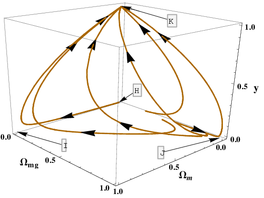
Fig. 5 shows the stability of critical points of the autonomous system (54)–(56) and (59) which is consistent with the results described in the Table 3. In Fig. 5 the points $H$ , $I$ , $J$ and $K$ are represented by the points $(\Omega_{m},\Omega_{\rm mg},y)\equiv(0,0,0)$ , $(\sim 1,0,0)$ , $(0,\sim 1,0)$ and $(0,0,\sim 1)$ respectively. We can see that all trajectories are going towards the attractor solution i.e, point $K$ . Fig. 5 and Table 3 show that the stability nature of this system is similar to the mass-varying massive gravity model without any conformal coupling.

Now let us compare these results with the minimal coupling case. For the minimal coupling case the fixed points and their nature of stability remains same but what changes is the $w_{\rm eff}$ for the matter dominated era and it changes to standard equation of state for matter. Also the $w_{\rm DE}$ approaches $0$ during matter dominated era. Contribution from massive gravity for all the cases behaves like matter giving rise to conventional equation of state for matter. So the coupling between matter and the field $\sigma$ actually removes the degeneracy between the two fixed points representing the matter dominated era and massive gravity dominated era.

As for the effect of the coupling on the evolution let us check the evolution of Hubble parameter. In Fig. 6 we have compared the evolution of the Hubble parameter for non minimal coupling case with the minimal coupling case and $\Lambda$ CDM model. We have used the available data for Hubble parameter $H(z)$ [71, 72, 73, 74, 75, 76, 77] and their $1\sigma$ error bars. From the data of $H(z)$ , we have calculated normalized Hubble parameter, i.e, $H/H_{0}$ where $H_{0}$ is the present value of the Hubble parameter. We have taken the value of $H_{0}$ from PLANCK 2013 results [70] and we have set $H_{0}=67.8~~\rm Km/Sec/Mpc$ . We have also estimated the error in $H/H_{0}$ from the given data. During the evolution we have set the present value of $\Omega_{m}$ to $0.315$ which is taken from the PLANCK 2013 results [70]. Fig. 6 shows that the evolution of the normalized Hubble parameter in $\Lambda$ CDM and minimally coupled case are very similar and also consistent with the available data. But the evolution of the Hubble parameter in the non minimally coupled case defers a lot from the $\Lambda$ CDM and minimally coupled case and is inconsistent with the present data. The deviations of the Hubble parameter changes the evolution of the matter, radiation and dark energy density parameters.

In the three cases discussed above, the limit $\beta\to 0$ is inconsistent which is obvious because in this limit we recover the original $dRGT$ nonlinear massive gravity which cannot give rise to the flat FLRW solution. The model under consideration can give rise to the flat FLRW cosmology with non minimal coupling only. To make the theory consistent with the $\beta\to 0$ limit we may consider a potential term of the $\sigma$ field in the massive gravity part.

III Non-minimal coupling in quasi-dilaton nonlinear massive gravity

In the models discussed in the preceding section, one needs a potential term to have a de Sitter solution irrespective of the conformal coupling term. Though the addition of the cubic galileon term gives a de Sitter solution without potential it is screened by the massive gravity dominated era which is also an attractor solution. So in any case massive gravity term in the varying mass nonlinear massive gravity does not give rise to a viable de Sitter solution. But in quasi-dilaton nonlinear massive gravity we get self acceleration from the massive gravity part [36, 37] without adding any potential term or a galileon. Now let us consider non-minimal coupling in quasi-dilaton nonlinear massive gravity [36] and consider the following action in the Einstein frame

$\displaystyle\mathcal{S}_{E}$	$\displaystyle=\int\rm d^{4}x\sqrt{-g}\bigg[\frac{M_{\textrm{Pl}}^{2}}{2}R-\frac{\omega}{2}g^{\mu\nu}\partial_{\mu}\sigma\partial_{\nu}\sigma$
	$\displaystyle-\frac{m^{2}M_{\textrm{Pl}}^{2}}{8}\left(4\,\mathcal{U}_{2}(\bar{\Bbbk})+\alpha_{3}\mathcal{U}_{3}(\bar{\Bbbk})+\alpha_{4}\mathcal{U}_{4}(\bar{\Bbbk})\right)\bigg]$
	$\displaystyle+\int d^{4}x\sqrt{-g}\mathcal{L}_{m}(A^{2}g_{\mu\nu},\psi)\,,$	(61)

where

\bar{\Bbbk}^{\mu}_{\nu}=\delta^{\mu}_{\nu}-e^{(\beta_{q}+\beta)\sigma/M_{\textrm{Pl}}}\sqrt{g^{\mu\alpha}\partial_{\alpha}\phi^{a}\partial_{\nu}\phi^{b}\eta_{ab}}\,,

(62)

with $\beta_{q}=1$ for the the quasi-dilaton nonlinear massive gravity described in [36]. Though for minimally coupled case ( $\beta=0$ ), we can absorb $\beta$ within the $\sigma$ field by redefining the field leaving the model unchanged.

The action (61) can be motivated from the Jordan frame action

$\displaystyle\mathcal{S}_{J}$	$\displaystyle=$	$\displaystyle\frac{M_{\textrm{Pl}}^{2}}{2}\int\rm d^{4}x\sqrt{-\tilde{g}}$	(63)
		$\displaystyle\bigg[\mathrm{e}^{2\beta\sigma/M_{\textrm{Pl}}}\left(\tilde{R}+\frac{(6\beta^{2}-\omega)}{M_{\textrm{Pl}}^{2}}\tilde{g}^{\mu\nu}\partial_{\mu}\sigma\partial_{\nu}\sigma\right)$
		$\displaystyle-\frac{m^{2}}{4}\mathrm{e}^{4\beta\sigma/M_{\textrm{Pl}}}\left(4\,\mathcal{U}_{2}(\Bbbk)+\alpha_{3}\mathcal{U}_{3}(\Bbbk)+\alpha_{4}\mathcal{U}_{4}(\Bbbk)\right)\bigg]$
		$\displaystyle+\sqrt{-\tilde{g}}\mathcal{L}_{m}(\tilde{g}_{\mu\nu},\psi)\,,$

where

\Bbbk^{\mu}_{\nu}=\delta^{\mu}_{\nu}-e^{\beta_{q}\sigma/M_{\textrm{Pl}}}\sqrt{g^{\mu\alpha}\partial_{\alpha}\phi^{a}\partial_{\nu}\phi^{b}\eta_{ab}}\,.

(64)

III.1 Lagrangian in the decoupling limit

The action (61) is same as the quasi-dilaton nonlinear massive gravity except we have a coupling between the $\sigma$ field with the matter field which will modify the continuity equation of matter. But even in the presence of the conformal coupling the decoupling limit (11) Lagrangian is same as the original model [36]. As for the local physics, we can have a contribution from the conformal coupling which comes from the matter conservation equation. But similar to the varying mass nonlinear massive gravity, the contribution from the conformal factor contains a factor like $\beta/M_{\textrm{Pl}}$ which makes the contribution vanishing in the decoupling limit. Thus the action (61) preserves the local physics through the Vainshtein mechanism.

III.2 Cosmology

By redefining the $\sigma$ field as $\sigma\to\sigma/(\beta_{q}+\beta)$ in the FLRW background (29) the action (61) becomes

	$\displaystyle\hskip-14.22636pt\mathcal{S}_{E}=3M_{Pl}^{2}\int{\rm d}t\biggl[-\frac{a\dot{a}^{2}}{N}+\frac{\omega_{0}}{6M_{\textrm{Pl}}^{2}}~\frac{a^{3}\dot{\sigma}^{2}}{N}$
	$\displaystyle\hskip 2.84526pt+m^{2}a^{3}\left(NG_{1}(\zeta)-\dot{f}aG_{2}(\zeta)\right)\biggr]+\mathcal{S}_{m}+\mathcal{S}_{r}\,,$		(65)

where for the Stückelberg scalars we consider the ansatz

\displaystyle\phi^{0}=f(t)\,,~~~\phi^{i}=x^{i}\,,

(66)

and we have defined

$\displaystyle G_{1}(\zeta)$	$\displaystyle=(1-\zeta)\biggl[2-\zeta+\frac{\alpha_{3}}{4}(1-\zeta)(4-\zeta)$
	$\displaystyle+\alpha_{4}(1-\zeta)^{2}\biggr]\,,$	(67)
$\displaystyle G_{2}(\zeta)$	$\displaystyle=\zeta(1-\zeta)\biggl[1+\frac{3}{4}\alpha_{3}(1-\zeta)+\alpha_{4}(1-\zeta)^{2}\biggr]\,,$	(68)
$\displaystyle\omega_{0}$	$\displaystyle=\frac{\omega}{(\beta_{q}+\beta)^{2}}\,,$	(69)

where $\zeta$ is defined as

\zeta=\frac{\mathrm{e}^{\sigma/M_{\textrm{Pl}}}}{a}.

(70)

In action (65) $\mathcal{S}_{m}$ and $\mathcal{S}_{r}$ represent the matter and radiation actions respectively. We should keep in mind that in the Einstein frame matter is coupled with the $\sigma$ field and this will modify the conservation equation of the matter.

Variation the action (61) with respect to $f$ gives the constraint equation (as an essential feature of any model of non-linear massive gravity)

\displaystyle G_{2}(\zeta)=\frac{C}{a^{4}}\,,

(71)

where $C$ is a constant of integration.

Varying the action (61) with respect to $N(t)$ and setting $N(t)=1$ at the end we get the Friedmann equation [37]

\displaystyle 3M_{\textrm{Pl}}^{2}H^{2}=\frac{\rho_{m}+\rho_{r}-3m^{2}M_{\textrm{Pl}}^{2}G_{1}}{1-\frac{\omega_{0}}{6}\Bigl(1-4\frac{G_{2}}{\zeta G_{2}^{\prime}}\Bigr)^{2}}\,,

(72)

where $\rho_{m}$ and $\rho_{r}$ are the matter and radiation energy density respectively. The primes in $G$ ’s denote derivatives with respect to their argument $\zeta$ .

Table 4: The real and physically meaningful critical points of the autonomous system (81)-(83), their existence conditions, the eigenvalues of the perturbation matrix, and the deduced stability conditions. We also present the corresponding values of the various density parameters, and the values of the observables: deceleration parameter

q

, total equation-of-state parameter

w_{\rm eff}

and dark energy equation-of-state parameter

w_{\rm DE}

Cr.P.	$\Omega_{r}$	$\Omega_{\Lambda}$	$\zeta$	$\Omega_{m}$	$\Omega_{\sigma}$	$q$	$w_{\rm eff}$	$w_{DE}$	Existence	Stability	Eigenvalues
									conditions
$P_{1}$	$1-3\omega_{0}/2$	0	0	0	$3\omega_{0}/2$	1	$1/3$	$1/3$	$0\leq\omega_{0}\leq 2/3$	Saddle point	$-4$ , 4, $1-3\beta_{0}$
										for all $\beta_{0}$
$P_{2}$	0	0	0	$1-3\omega_{0}/2$	$3\omega_{0}/2$	$(1+3\beta_{0})/2$	$\beta_{0}$	$2\beta_{0}/3\omega_{0}$	$0\leq\omega_{0}\leq 2/3$	Saddle point	$-4$ , $3+3\beta_{0}$ ,
										for $\beta_{0}>-1$	$-1+3\beta_{0}$
$P_{3}$	0	$1-3\omega_{0}/2$	0	0	$3\omega_{0}/2$	-1	-1	-1	$0\leq\omega_{0}\leq 2/3$	Attractor	$-4$ , $-4$ ,
										for $\beta_{0}>-1$	$-3(1+\beta_{0})$
$P_{4\pm}$	$1-\omega_{0}/6$	0	$\zeta_{\pm}$	0	$\omega_{0}/6$	1	$1/3$	1/3	$0\leq\omega_{0}\leq 6$ ,	Saddle point	$-4$ ,4, $1+\beta_{0}$
									$0\leq\zeta_{\pm}$	for all $\beta_{0}$
$P_{5\pm}$	0	0	$\zeta_{\pm}$	$1-\omega_{0}/6$	$\omega_{0}/6$	$(1-\beta_{0})/2$	$-\beta_{0}/3$	$-2\beta_{0}/\omega_{0}$	$0\leq\omega_{0}\leq 6$ ,	Saddle point	$-4$ , $-1-\beta_{0}$ ,
									$0\leq\zeta_{\pm}$	for $\beta_{0}<3$	$3-\beta_{0}$
$P_{6\pm}$	0	$1-\omega_{0}/6$	$\zeta_{\pm}$	0	$\omega_{0}/6$	-1	-1	-1	$0\leq\omega_{0}\leq 6$ ,	Attractor	$-4$ , $-4$ , $-3+\beta_{0}$
									$0\leq\zeta_{\pm}$	for $\beta_{0}<3$
$P_{7}$	0	0	1	$1-\omega_{0}/6$	$\omega_{0}/6$	$(1-\beta_{0})/2$	$-\beta_{0}/3$	$-2\beta_{0}/\omega_{0}$	$0\leq\omega_{0}\leq 6$	Attractor	$-4$ , $-1-\beta_{0}$ ,
										for $\beta_{0}>-1$	$-1-\beta_{0}$
$P_{8}$	$\Omega_{r}$	$1-\omega_{0}/6$	$1$	0	$\omega_{0}/6$	$1$	$1/3$	$1/3$	$0\leq\omega_{0}\leq 6$	Saddle	$-4$ , $1+\beta_{0}$ ,0
		- $\Omega_{r}$								for $\beta_{0}>-1$

Similarly, variation with respect to $\sigma$ gives the dilaton evolution equation

\frac{\omega_{0}}{a^{3}}\frac{d}{dt}(a^{3}\dot{\sigma})-3M_{\textrm{Pl}}m^{2}\zeta\left(G_{1}^{\prime}(\zeta)-a\dot{f}G_{2}^{\prime}(\zeta)\right)=-\frac{\beta_{0}}{M_{\textrm{Pl}}}\rho_{m}\,,

(73)

where

\beta_{0}=\frac{\beta}{\beta_{q}+\beta}\,.

(74)

Continuity equations for matter and radiation are same as Eqs. (43) and (44), respectively. Now using Eq. (71) we can get an effective pressure for the matter phase which is given by

p_{m(\rm eff)}=-\frac{\beta_{0}}{3}\left(1-\frac{4G_{2}}{\zeta G_{2}^{\prime}}\right)\,.

(75)

Here we can also have an effective pressure for the matter phase which is the contribution from the conformal coupling. Now let us study how this effective pressure affects the cosmology of the model. And to study this we need to form an autonomous system. Let us first introduce the density parameters

$\displaystyle\Omega_{m}$	$\displaystyle=\frac{\rho_{m}}{3M_{\textrm{Pl}}^{2}H^{2}}\,,$	(76)
$\displaystyle\Omega_{r}$	$\displaystyle=\frac{\rho_{r}}{3M_{\textrm{Pl}}^{2}H^{2}}\,,$	(77)
$\displaystyle\Omega_{\Lambda}$	$\displaystyle=-\frac{m^{2}}{H^{2}}G_{1}\,,$	(78)
$\displaystyle\Omega_{\sigma}$	$\displaystyle=\frac{\omega_{0}}{6}\left(1-4\frac{G_{2}}{\zeta G_{2}^{\prime}}\right)^{2}\,,$	(79)

with which we can rewrite the Friedmann equation (72) as

\displaystyle\Omega_{m}+\Omega_{r}+\Omega_{\Lambda}+\Omega_{\sigma}=1\,.

(80)

We can now transform the above cosmological system into its autonomous form, using only the dimensionless variables $\Omega_{r}$ , $\Omega_{\Lambda}$ and $\xi$ , while (80) will be used to eliminate $\Omega_{m}$ . Doing so we obtain

$\displaystyle\frac{{\rm d}\Omega_{r}}{{\rm d}\ln a}$	$\displaystyle=-2\Omega_{r}\left(2+\frac{\dot{H}}{H^{2}}\right)\,,$	(81)
$\displaystyle\frac{{\rm d}\Omega_{\Lambda}}{{\rm d}\ln a}$	$\displaystyle=-2\Omega_{\Lambda}\left(2\frac{G_{2}G_{1}^{\prime}}{G_{1}G_{2}^{\prime}}+\frac{\dot{H}}{H^{2}}\right)\,,$	(82)
$\displaystyle\frac{{\rm d}\xi}{{\rm d}\ln a}$	$\displaystyle=-4\frac{G_{2}}{G_{2}^{\prime}}\,,$	(83)

where the combination $\frac{\dot{H}}{H^{2}}$ can be acquired differentiating the Friedmann equation (72) as

	$\displaystyle\hskip-28.45274pt\frac{\dot{H}}{H^{2}}=\frac{1}{6-\omega_{0}\left(1-4\frac{G_{2}}{\zeta G_{2}^{\prime}}\right)^{2}}$
	$\displaystyle\times\Biggl\{-9\Omega_{m}\left[1-\frac{\beta_{0}}{3}\left(1-\frac{4G_{2}}{\zeta G_{2}^{\prime}}\right)\right]-12\Omega_{r}$
	$\displaystyle-12\frac{G_{2}}{G_{2}^{\prime}}\left[\frac{G_{1}^{\prime}}{G_{1}}\Omega_{\Lambda}+\frac{\omega_{0}}{6}\frac{\rm d}{{\rm d}\zeta}\left(1-4\frac{G_{2}}{\zeta G_{2}^{\prime}}\right)^{2}\right]\Biggr\}\,.$		(84)

The effective equation of state parameter $w_{\rm eff}$ , the deceleration parameter $q$ and the dark energy equation of state parameter $w_{\rm DE}$ are defined as

$\displaystyle w_{\rm eff}$	$\displaystyle\hskip-1.99997pt=\hskip-1.99997pt$	$\displaystyle-1-\frac{2}{3}\frac{\dot{H}}{H^{2}}\,,$	(85)
$\displaystyle q$	$\displaystyle\hskip-1.99997pt=\hskip-1.99997pt$	$\displaystyle-1-\frac{\dot{H}}{H^{2}}=\frac{1}{2}+\frac{3}{2}w_{\rm eff}\,,$	(86)
$\displaystyle w_{\rm DE}$	$\displaystyle\hskip-1.99997pt=\hskip-1.99997pt$	$\displaystyle\frac{w_{\rm eff}-w_{r}\Omega_{r}}{\Omega_{\Lambda}+\Omega_{\sigma}}\,,$	(87)

where the combination $\dot{H}/H^{2}$ is given by Eq. (84) and $w_{r}=1/3$ .

The critical points of the above autonomous system are extracted setting the left hand sides of equations (81)–(83) to zero. In particular, equation (83) implies that at the critical points $G_{2}(\zeta)=0$ , which according to (68) gives $\zeta=0$ , $\zeta=1$ and

\displaystyle\zeta_{\pm}

\displaystyle=1+\frac{3\alpha_{3}\pm\sqrt{9\alpha_{3}^{2}-64\alpha_{4}}}{8\alpha_{4}}\,.

(88)

To be physical, the critical points have to possess $0\leq\Omega_{r}\leq 1$ , $0\leq\Omega_{\Lambda}+\Omega_{\sigma}\leq 1$ , $0\leq\zeta$ and of course $\zeta\in{\cal{R}}$ . Now, in order for $\zeta_{\pm}\in{\cal{R}}$ , we require $9\alpha_{3}^{2}-64\alpha_{4}\geq 0$ while $0\leq\zeta$ leads to the necessary conditions for $\alpha$ ’s using Eq. (88). All the fixed points and their nature of stability along with the values of effective equation of state ( $w_{\rm eff}$ ) and dark energy equation of state ( $w_{\rm DE}$ ) are given in Table 4. Fig. 7 shows the trajectories on the $\Omega_{m}$ – $\Omega_{\rm DE}$ plane. For $\zeta=1$ the matter phase is an attractor point which is represented in the Fig. 7 by the purple lines. But for $\zeta=0$ or $\zeta=\zeta_{\pm}$ we have late time acceleration as the attractor solution and it is represented in the Fig. 7 by the red lines.

To have viable thermal history of the universe we need to have $\Omega_{\rm DE}\leq 0.01$ during the radiation dominated era which gives a constraint on the value of $\omega_{0}$ ( $\omega_{0}\leq 0.02/3$ ) for $\zeta=0$ and $\omega_{0}\leq 0.06$ for the point $\zeta=\zeta_{\pm}$ . Though this is a rough estimation on the constraint on $\omega_{0}$ . We can have full constraint on $\omega_{0}$ by using the cosmological data sets. We also see from Table 4 that the conditions for stability of the fixed points and the values of the dimensionless variables do not depend on $\alpha$ ’s. But to have $\Omega_{\Lambda}>0$ for the points $P_{3}$ and $P_{6\pm}$ we can have $2+\alpha_{3}+\alpha_{4}<0$ for the point $P_{3}$ , $\alpha_{3}>0$ and $0<\alpha_{4}<\alpha_{3}^{2}/8$ for the point $P_{6+}$ and $\alpha_{3}<0$ and $0<\alpha_{4}<\alpha_{3}^{2}/8$ for the point $P_{6-}$ . These conditions are needed to have viable evolution of the cosmological parameters. But since the stability does not imply explicit dependence on $\alpha$ ’s, we can not have constraints on $\alpha$ ’s from the the observational data sets [37] because maintaining the conditions on $\alpha$ ’s if we change their values, cosmology does not change appreciably. Fig. 8 depicts that the model under consideration gives proper cosmological sequences starting from the radiation dominated era to the late time cosmic acceleration maintaining the proper matter dominated era. Cosmological evolution of the effective equation of state ( $w_{\rm eff}$ ) and dark energy equation of state ( $w_{\rm DE}$ ) are shown in Fig. 9 which clearly shows that the present era is dark energy dominated.

It is clear from Table 4 that due to the presence of conformal coupling, we have a different evolution of the dark energy equation of state ( $w_{\rm DE}$ ) than the one in the minimally coupled quasi-dilaton nonlinear massive gravity [24, 37]. For the case under consideration, $w_{\rm DE}$ has a non zero value for $\beta_{0}\neq 0$ during matter dominated era (see Fig. 9). This figure is plotted such that we can reach the attractor point $P_{3}$ during the late time. Table 4 also tells that for point $P_{3}$ , $\beta_{0}/\omega_{0}\sim 1$ , during matter era ( $w_{\rm DE}\sim 2/3$ ) which is confirmed numerically (see Fig. 9). In minimally coupled case, the value of $w_{\rm DE}$ during the matter era is zero [37] which can be checked from the Table 4 by putting $\beta_{0}=0$ . Hence looking at the evolution of $w_{\rm DE}$ , we can differentiate between the minimally coupled and non-minimally coupled quasi-dilaton nonlinear massive gravity. It is really interesting to note (see Table 4) that in case of the attractor represented by $P_{6\pm}$ , the parameter $w_{\rm DE}$ can reach super negative values before reaching de Sitter during evolution depending upon the values of $\beta_{0}$ and $\omega_{0}$ . We also emphasize that the current data allows phantom acceleration which is realized in our model as a transient phenomenon $-$ a phantom phase without a phantom field. The non-minimal coupling is responsible for the transient phantom behavior, see Fig. 10.

III.3 Observational Constraints

We now get to the investigations on constraints we can have on the model parameters from the observational data sets. The model under consideration has the parameters $\alpha_{3}$ , $\alpha_{4}$ , $\beta_{0}$ , $\omega_{0}$ , $m$ , $\Omega_{m0}$ , $C$ and $H_{0}$ . To obtain the observational constraints on the model parameters we have used the observational data sets of Type Ia Supernovae (SNIa) [81], Baryon Acoustic Oscillations (BAO) [83, 84, 85, 86], and CMB shift parameter [79] and Hubble parameter data [71, 72, 73, 74, 75, 76, 77].

Since we have many parameters we fix some them from the stability conditions. It is clear from Table 4 that the fixed points and their conditions for stability do not depend on $\alpha_{3}$ and $\alpha_{4}$ . Thus the cosmology does not depend on the $\alpha$ ’s and consequently we can not get any constraint on $\alpha$ ’s. But we can have some conditions on $\alpha$ ’s from the consideration that at the fixed point $\Omega_{\Lambda}>0$ . From these conditions we can fix some values for $\alpha_{3}$ and $\alpha_{4}$ . One should note that maintaining the conditions on $\alpha$ ’s if one change their values then the cosmology does not change and that is why we can not have any constraint on the $\alpha$ ’s [37]. So we fix $\alpha_{3}=1$ and $\alpha_{4}=0.115$ which respect the conditions on $\alpha$ ’s for the point $P_{6+}$ . We also fix the present value of the Hubble parameter $H_{0}$ from the Planck 2013 result [70]. Since the autonomous system and the fixed points do not depend on the value of $C$ , we can not also derive any constraint on it. Also the numerical evolution of the autonomous system does not depend on graviton mass $m$ but we can have an estimation of the value of $m$ from the evolution of the Hubble parameter for the best fit values of the other model parameters. So finally we are left with three model parameters $\beta_{0}$ , $\omega_{0}$ and $\Omega_{m0}$ .

Total $\chi^{2}$ is defined in Eq. (89). Along with the total $\chi^{2}$ which incorporates the recent Planck result, we have also used the estimation on the present value of matter density parameter ( $\Omega_{m0}$ ) as a prior information where mean value of $\Omega_{m0}$ lies at 0.315. We have taken the maximum uncertainty of $\Omega_{m0}$ measurement in Planck results which is 0.018. The detailed procedure of data analysis is given in Appendix. We have varied the parameter $\beta_{0}$ from $-0.2$ to $0.1$ , parameter $\omega_{0}$ from $-2.5$ to $1$ and $\Omega_{m0}$ from $0.24$ to $0.36$ . Minimizing the total $\chi^{2}$ , we get the best fit values for the parameters. For this model best fit values of the considered model parameters are $\beta_{0}\approx-0.04$ , $\omega_{0}\approx-0.5$ and $\Omega_{m0}\approx 0.3$ .

Fig. 11 shows the 1 $\sigma$ and 2 $\sigma$ contours on $\beta_{0}-\Omega_{m0}$ plane after marginalizing on the parameter $\omega_{0}$ . Similarly Figs. 12 and 13 show the 1 $\sigma$ and 2 $\sigma$ contours on $\omega_{0}-\Omega_{m0}$ and $\beta_{0}-\omega_{0}$ planes respectively after marginalizing on $\beta_{0}$ and $\Omega_{m0}$ respectively. Fig. 11 shows that very small value of $\beta_{0}$ is allowed. Fig. 12 shows the consistency with the results depicted in Table 4 which tells us that very small positive value of $\omega_{0}$ is allowed to have viable thermal history of the universe. This figure also tells us that negative values of $\omega_{0}$ can also give viable cosmology corresponding to phantom phase in the evolution of the dark energy component.

Next from Eq. (74), we observe that if we put the conformal coupling constant $\beta=0$ then $\beta_{0}$ also becomes zero and the theory reduces to the original quasi-dilaton nonlinear massive gravity [36]. But observationally we found that though $\beta_{0}=0$ is allowed within the $1\sigma$ confidence level we also have some non zero values of $\beta_{0}$ allowed within the $1\sigma$ confidence level; the best fit value of $\beta_{0}$ is non zero. Given the present data. However, given the present data, we can not claim which one of them, minimal/non minimal coupling is more favored. We find that generally small numerical values of non minimal coupling in the quasi-dilaton nonlinear massive gravity are favored.

IV Conclusions

In this paper, we have investigated the effect of non-minimal coupling in (extended) massive gravity theories. As our first example, we have studied the case of mass varying nonlinear massive gravity in Brans-Dicke framework. In this scenario, the conformal coupling is responsible for making the graviton mass varying. General theory of relativity is restored by Vainshtein screening in this case such that conformal coupling does not affect the local physics.

Our analysis shows that if we do not complement the $\sigma$ Lagrangian by potential or by a non linear galileon Lagrangian, the conformal coupling alone can not give rise to de Sitter solution. It gives rise to an effective pressure of matter such that the matter dominated era is a late time attractor. And as a result we do not have the required equation of state at late times.

We next invoke cubic galileon Lagrangian and potential for the $\sigma$ field. Adding cubic galileon alone leads to a de Sitter solution as an attractor of the dynamics but simultaneously we also have matter dominated era as an attractor solution. We have bi-stability in this case and while following the thermal history of the universe, we can not reach the de Sitter phase because the latter is blocked by the matter era. Only by invoking unnatural fine tunings, we can realize the de Sitter phase which is not desirable. However, replacing the galileon term by a potential of the $\sigma$ field, it is possible to obtain a stable de Sitter solution. It is interesting that the potential term turns the matter phase into a saddle point under certain conditions. Though this scenario can give us a right sequence of different cosmological eras, we can not get rid of the problem of having a constant non zero equation of state for the matter phase. Evolution of the normalized Hubble parameter in this model is compared to that of the minimal case and the $\Lambda$ CDM using the available data and it is found that the evolution of the Hubble parameter in this model does not fit with data while the case of minimal coupling is consistent with observations. Thus the conformal coupling appreciably changes the evolution of the Hubble parameter.

Next we studied the effect of conformal coupling for quasi-dilaton nonlinear massive gravity. In this case we have considered an extra coupling $\beta_{q}$ which makes the model consistent in the limit $\beta\to 0$ . We have performed detailed dynamical analysis for this model. In this setting, we find a de Sitter solution as a late time attractor. We have shown that model under consideration gives rise to viable cosmology. From the dynamical analysis, it is found that the fixed points and their conditions for stability do not depend upon the numerical values of the parameters, $\alpha_{3}$ and $\alpha_{4}$ thereby cosmology is not sensitive to these parameters. Also we do not find any dependency of cosmological dynamics on the graviton mass $m$ and parameter $C$ as these two parameters do not appear in the dynamical system explicitly.

We have also analyzed the observational constraints on the model parameters $\beta$ , $\omega$ and $\Omega_{mo}$ . It is found that both the parameters $\beta$ and $\omega$ are preferred to have small numerical values both positive and negative allowed within the 2 $\sigma$ confidence level.

Our investigations reveal that not any mass-varying non linear massive gravity scheme can give rise to a viable cosmology at the background level. The quasi-dilaton model turns out to be very generic in the list of such models. And our analysis shows that the non minimal coupling in the quasi-dilaton nonlinear massive gravity can give rise to viable cosmology. From the observational data analysis it is found that small value of the conformal coupling is favored. It is remarkable that the introduction of non-minimal coupling in quasi-dilaton model can give rise to a transient phantom phase allowed by the recent data with certain preference [70]. This is a generic feature of the scenario that allows to realize phantom behavior without a phantom field. Future observations might distinguish the quasi-dilaton model from its counter part with non minimal coupling considered in this paper.

Last but not least, It will be important to investigate whether the non-minimal coupling alone (without the extra terms introduced in [40] which do not disturb background) can ensure the stability of the background. If it does not, it will be important to incorporate the extra terms along with non minimal coupling and investigate the phantom behavior and stability issues. We defer this work for our future investigations.

Acknowledgements.

We thank T. Koivisto for useful comments. M.W.H. acknowledges the funding from CSIR, govt. of India. The work is supported in part by the JSPS Grant-in-Aid for Young Scientists (B) # 25800136 (K.B.) and that for Scientific Research (S) # 22224003 and (C) # 23540296 (S.N.). M.S. thanks Kobayashi-Maskawa Institute (KMI) for the Origin of Particles and the Universe for hosting him as a senior JSPS fellow (L-12522), where the work was initiated. He also thanks the Eurasian International Center for Theoretical Physics, Eurasian National University, Astana 010008, Kazakhstan, where the work was completed. R.M. thanks KMI for hospitality during his visit to Nagoya, during KMI-IEEC Joint International Workshop – Inflation, Dark Energy, and Modified Gravity in the PLANCK Era. He acknowledges fruitful discussions with S. Nojiri and K. Bamba on the related theme.

Table 5: Values of

\frac{d_{A}(z_{\star})}{D_{V}(Z_{BAO})}

for different values of

z_{BAO}

$z_{BAO}$	0.106	0.2	0.35	0.44	0.6	0.73
$\frac{d_{A}(z_{\star})}{D_{V}(Z_{BAO})}$	$30.95\pm 1.46$	$17.55\pm 0.60$	$10.11\pm 0.37$	$8.44\pm 0.67$	$6.69\pm 0.33$	$5.45\pm 0.31$

Appendix A Observational Data Analysis

Here we briefly review the sources of observational constraints used in this manuscript, namely Type Ia Supernovae constraints, BAO, CMB and data of Hubble parameter. The total $\chi^{2}$ defined as

\displaystyle\chi_{\rm tot}^{2}=\chi_{\rm SN}^{2}+\chi_{\rm Hub}^{2}+\chi_{\rm BAO}^{2}+\chi_{\rm CMB}^{2}\,,

(89)

where the individual $\chi^{2}_{i}$ for every data set is calculated as follows.

Table 6: Hubble parameter versus redshift data [78].

$z$	$H(z)$	$\sigma_{H}$	Reference
	(km/s/Mpc)	(km/s/Mpc)
0.070	69	19.6	[74]
0.100	69	12	[71]
0.120	68.6	26.2	[74]
0.170	83	8	[71]
0.179	75	4	[73]
0.199	75	5	[73]
0.200	72.9	29.6	[74]
0.270	77	14	[71]
0.280	88.8	36.6	[74]
0.350	76.3	5.6	[77]
0.352	83	14	[73]
0.400	95	17	[71]
0.440	82.6	7.8	[75]
0.480	97	62	[72]
0.593	104	13	[73]
0.600	87.9	6.1	[75]
0.680	92	8	[73]
0.730	97.3	7.0	[75]
0.781	105	12	[73]
0.875	125	17	[73]
0.880	90	40	[72]
0.900	117	23	[71]
1.037	154	20	[73]
1.300	168	17	[71]
1.430	177	18	[71]
1.530	140	14	[71]
1.750	202	40	[71]
2.300	224	8	[76]

a. $\chi^{2}$ for Type Ia Supernovae

In order to incorporate Type Ia constraints we use the Union2.1 data compilation [81] of 580 data points. The relevant observable is the distance modulus $\mu$ which is defined as $\mu=m-M=5\log D_{L}+\mu_{0}$ , where $m$ and $M$ are the apparent and absolute magnitudes of the Supernovae, $D_{L}(z)$ is the luminosity distance $D_{L}(z)=(1+z)\int_{0}^{z}\frac{H_{0}dz^{\prime}}{H(z^{\prime})}$ and $\mu_{0}=5\log\left(\frac{H_{0}^{-1}}{\rm Mpc}\right)+25$ is a nuisance parameter that should be marginalized. The corresponding $\chi^{2}$ writes as

\displaystyle\chi_{\rm SN}^{2}(\mu_{0},\theta)=\sum_{i=1}^{580}\frac{\left[\mu_{th}(z_{i},\mu_{0},\theta)-\mu_{obs}(z_{i})\right]^{2}}{\sigma_{\mu}(z_{i})^{2}}\,,

(90)

where $\mu_{obs}$ denotes the observed distance modulus while $\mu_{th}$ the theoretical one, and $\sigma_{\mu}$ is the uncertainty in the distance modulus. Additionally, $\theta$ denotes any parameter of the specific model at hand. Finally, marginalizing $\mu_{0}$ following [82] we obtain

\displaystyle\chi_{\rm SN}^{2}(\theta)=A(\theta)-\frac{B(\theta)^{2}}{C(\theta)}\,,

(91)

with

		$\displaystyle A(\theta)=\sum_{i=1}^{580}\frac{\left[\mu_{th}(z_{i},\mu_{0}=0,\theta)-\mu_{obs}(z_{i})\right]^{2}}{\sigma_{\mu}(z_{i})^{2}}\,,$		(92)
		$\displaystyle B(\theta)=\sum_{i=1}^{580}\frac{\mu_{th}(z_{i},\mu_{0}=0,\theta)-\mu_{obs}(z_{i})}{\sigma_{\mu}(z_{i})^{2}}\,,$		(93)
		$\displaystyle C(\theta)=\sum_{i=1}^{580}\frac{1}{\sigma_{\mu}(z_{i})^{2}}\,.$		(94)

d. $\chi^{2}$ for Hubble data

Along with the present value of the Hubble parameter we have 29 data points of Hubble parameter given in Table 6. To use the data of Hubble parameter we have used the normalized Hubble parameter defined as, $h=H/H_{0}$ . We fix the value of $H_{0}$ from [70]. Error in normalized Hubble parameter is given by,

\sigma_{h}=\left(\frac{\sigma_{H}}{H}+\frac{\sigma_{H_{0}}}{H_{0}}\right)h\,,

(95)

where $\sigma_{H}$ is the error in Hubble parameter and $\sigma_{H_{0}}$ is the error in present value of the Hubble parameter.

The $\chi^{2}$ for the normalized Hubble parameter data is given by,

\displaystyle\chi_{\rm Hub}^{2}(\mu_{0},\theta)=\sum_{i=1}^{29}\frac{\left[h_{\rm th}(z_{i},\theta)-h_{\rm obs}(z_{i})\right]^{2}}{\sigma_{H}(z_{i})^{2}}\,,

(96)

where $h_{\rm th}$ and $h_{\rm obs}$ are the theoretical and observed values of the normalized Hubble parameter.

b. $\chi^{2}$ for Baryon Acoustic Oscillation (BAO)

We use BAO data from [83, 84, 85, 86], that is of $\frac{d_{A}(z_{\star})}{D_{V}(Z_{BAO})}$ , where $z_{\star}$ is the decoupling time given by $z_{\star}\approx 1091$ , the co-moving angular-diameter distance $d_{A}(z)=\int_{0}^{z}\frac{dz^{\prime}}{H(z^{\prime})}$ and $D_{V}(z)=\left(d_{A}(z)^{2}\frac{z}{H(z)}\right)^{\frac{1}{3}}$ is the dilation scale [87]. th required data are depicted in Table 5.

In order to calculate $\chi_{\mathrm{BAO}}^{2}$ for BAO data we follow the procedure described in Ref. [88], where it is defined as,

\chi_{\rm BAO}^{2}=X_{\rm BAO}^{T}C_{\rm BAO}^{-1}X_{\rm BAO}\,,

(97)

with

X_{\rm BAO}=\left(\begin{array}[]{c}\frac{d_{A}(z_{\star})}{D_{V}(0.106)}-30.95\\ \frac{d_{A}(z_{\star})}{D_{V}(0.2)}-17.55\\ \frac{d_{A}(z_{\star})}{D_{V}(0.35)}-10.11\\ \frac{d_{A}(z_{\star})}{D_{V}(0.44)}-8.44\\ \frac{d_{A}(z_{\star})}{D_{V}(0.6)}-6.69\\ \frac{d_{A}(z_{\star})}{D_{V}(0.73)}-5.45\end{array}\right)\,,

(98)

and the inverse covariance matrix reads as

\displaystyle C^{-1}=\left(\begin{array}[]{cccccc}0.48435&-0.101383&-0.164945&-0.0305703&-0.097874&-0.106738\\ -0.101383&3.2882&-2.45497&-0.0787898&-0.252254&-0.2751\\ -0.164945&-2.45499&9.55916&-0.128187&-0.410404&-0.447574\\ -0.0305703&-0.0787898&-0.128187&2.78728&-2.75632&1.16437\\ -0.097874&-0.252254&-0.410404&-2.75632&14.9245&-7.32441\\ -0.106738&-0.2751&-0.447574&1.16437&-7.32441&14.5022\end{array}\right)\,.

c. $\chi^{2}$ for CMB shift parameter

We use the CMB shift parameter

\displaystyle R=H_{0}\sqrt{\Omega_{m0}}\int_{0}^{1089}\frac{dz^{\prime}}{H(z^{\prime})}\,,

(105)

following [79]. The corresponding $\chi_{\rm CMB}^{2}$ is defined as,

\displaystyle\chi_{\rm CMB}^{2}(\theta)=\frac{(R(\theta)-R_{0})^{2}}{\sigma^{2}}\,,

(106)

with $R_{0}=1.725\pm 0.018$ and $R(\theta)$ [79].

References

[1] E. J. Copeland, M. Sami and S. Tsujikawa, Int. J. Mod. Phys. D 15, 1753 (2006) [hep-th/0603057].
[2] S. Nojiri and S. D. Odintsov, Phys. Rept. 505, 59 (2011) [arXiv:1011.0544 [gr-qc]]; eConf C0602061, 06 (2006) [Int. J. Geom. Meth. Mod. Phys. 4, 115 (2007)] [arXiv:hep-th/0601213].
[3] T. Clifton, P. G. Ferreira, A. Padilla and C. Skordis, Phys. Rept. 513, 1 (2012) [arXiv:1106.2476 [astro-ph.CO]].
[4] K. Bamba, S. Capozziello, S. Nojiri and S. D. Odintsov, Astrophys. Space Sci. 342, 155 (2012) [arXiv:1205.3421 [gr-qc]].
[5] J. Khoury and A. Weltman, Phys. Rev. Lett. 93, 171104 (2004) [astro-ph/0309300].
[6] J. Khoury and A. Weltman, Phys. Rev. D 69, 044026 (2004) [astro-ph/0309411].
[7] A. I. Vainshtein, Phys. Lett. B 39, 393 (1972).
[8] M. A. Luty, M. Porrati and R. Rattazzi, JHEP 0309, 029 (2003) [hep-th/0303116].
[9] A. Nicolis and R. Rattazzi, JHEP 0406, 059 (2004) [hep-th/0404159].
[10] A. Nicolis, R. Rattazzi and E. Trincherini, Phys. Rev. D 79, 064036 (2009) [arXiv:0811.2197 [hep-th]].
[11] K. Van Acoleyen and J. Van Doorsselaere, Phys. Rev. D 83, 084025 (2011) [arXiv:1102.0487 [gr-qc]].
[12] M. Fierz, W. Pauli, Proc. Roy. Soc. Lond. A173, 211 (1939).
[13] H. van Dam and M. J. G. Veltman, Nucl. Phys. B 22, 397 (1970).
[14] V. I. Zakharov, JETP Lett. 12, 312 (1970) [Pisma Zh. Eksp. Teor. Fiz. 12, 447 (1970)].
[15] D. G. Boulware, S. Deser, Phys. Rev. D6, 3368 (1972).
[16] C. de Rham and G. Gabadadze, Phys. Rev. D 82, 044020 (2010) [arXiv:1007.0443 [hep-th]].
[17] C. de Rham, G. Gabadadze and A. J. Tolley, Phys. Rev. Lett. 106, 231101 (2011) [arXiv:1011.1232 [hep-th]].
[18] K. Hinterbichler, Rev. Mod. Phys. 84, 671 (2012) [arXiv:1105.3735 [hep-th]].
[19] S. F. Hassan and R. A. Rosen, Phys. Rev. Lett. 108, 041101 (2012) [arXiv:1106.3344 [hep-th]].
[20] S. Deser and A. Waldron, Phys. Rev. Lett. 110, 111101 (2013) [arXiv:1212.5835 [hep-th]].
[21] K. Koyama, G. Niz and G. Tasinato, Phys. Rev. Lett. 107, 131101 (2011) [arXiv:1103.4708 [hep-th]].
[22] K. Koyama, G. Niz and G. Tasinato, Phys. Rev. D 84, 064033 (2011) [arXiv:1104.2143 [hep-th]].
[23] G. D’Amico, C. de Rham, S. Dubovsky, G. Gabadadze, D. Pirtskhalava and A. J. Tolley, Phys. Rev. D 84, 124046 (2011) [arXiv:1108.5231 [hep-th]].
[24] A. De Felice, A. E. Gumrukcuoglu and S. Mukohyama, Phys. Rev. Lett. 109, 171101 (2012) [arXiv:1206.2080 [hep-th]].
[25] N. Khosravi, G. Niz, K. Koyama and G. Tasinato, JCAP 1308, 044 (2013) [arXiv:1305.4950 [hep-th]].
[26] A. E. Gumrukcuoglu, C. Lin and S. Mukohyama, Phys. Lett. B 717 (2012) 295 [arXiv:1206.2723 [hep-th]].
[27] A. De Felice, A. E. Gumrukcuoglu, C. Lin and S. Mukohyama, JCAP 1305, 035 (2013) [arXiv:1303.4154 [hep-th]].
[28] A. E. Gumrukcuoglu, C. Lin and S. Mukohyama, JCAP 1111, 030 (2011) [arXiv:1109.3845 [hep-th]].
[29] A. E. Gumrukcuoglu, C. Lin and S. Mukohyama, JCAP 1203, 006 (2012) [arXiv:1111.4107 [hep-th]].
[30] P. Jain and J. P. Ralston, Mod. Phys. Lett. A 14, 417 (1999) [astro-ph/9803164].
[31] Q. -G. Huang, Y. -S. Piao and S. -Y. Zhou, Phys. Rev. D 86, 124014 (2012) [arXiv:1206.5678 [hep-th]].
[32] Q. -G. Huang, K. -C. Zhang and S. -Y. Zhou, JCAP 1308, 050 (2013) [arXiv:1306.4740 [hep-th]].
[33] Y. -F. Cai, C. Gao and E. N. Saridakis, JCAP 1210, 048 (2012) [arXiv:1207.3786 [astro-ph.CO]].
[34] E. N. Saridakis, Class. Quant. Grav. 30, 075003 (2013) [arXiv:1207.1800 [gr-qc]].
[35] G. Leon, J. Saavedra and E. N. Saridakis, Class. Quant. Grav. 30, 135001 (2013) [arXiv:1301.7419 [astro-ph.CO]].
[36] G. D’Amico, G. Gabadadze, L. Hui and D. Pirtskhalava, Phys. Rev. D 87, 064037 (2013) arXiv:1206.4253 [hep-th].
[37] R. Gannouji, M. W. Hossain, M. Sami and E. N. Saridakis, Phys. Rev. D 87, 123536 (2013) [arXiv:1304.5095 [gr-qc]].
[38] A. E. Gumrukcuoglu, K. Hinterbichler, C. Lin, S. Mukohyama and M. Trodden, Phys. Rev. D 88, 024023 (2013) [arXiv:1304.0449 [hep-th]].
[39] G. D’Amico, G. Gabadadze, L. Hui and D. Pirtskhalava, Class. Quant. Grav. 30, 184005 (2013) [arXiv:1304.0723 [hep-th]].
[40] A. De Felice and S. Mukohyama, Phys. Lett. B 728, 622 (2014) [arXiv:1306.5502 [hep-th]].
[41] A. De Felice, A. E. Gumrukcuoglu and S. Mukohyama, arXiv:1309.3162 [hep-th].
[42] M. Andrews, G. Goon, K. Hinterbichler, J. Stokes and M. Trodden, Phys. Rev. Lett. 111, 061107 (2013) [arXiv:1303.1177 [hep-th]].
[43] M. Andrews, K. Hinterbichler, J. Stokes and M. Trodden, Class. Quant. Grav. 30, 184006 (2013) [arXiv:1306.5743 [hep-th]].
[44] K. Hinterbichler, J. Stokes and M. Trodden, Phys. Lett. B 725, 1 (2013) [arXiv:1301.4993 [astro-ph.CO]].
[45] G. D’Amico, Phys. Rev. D 86, 124019 (2012) [arXiv:1206.3617 [hep-th]].
[46] P. Guarato and R. Durrer, arXiv:1309.2245 [gr-qc].
[47] Z. Haghani, H. R. Sepangi and S. Shahidi, Phys. Rev. D 87, 124014 (2013) [arXiv:1303.2843 [gr-qc]].
[48] Y. Akrami, T. S. Koivisto, D. F. Mota and M. Sandstad, arXiv:1306.0004 [hep-th].
[49] N. Tamanini, E. N. Saridakis and T. S. Koivisto, arXiv:1307.5984 [hep-th].
[50] S. F. Hassan and R. A. Rosen, JHEP 1202, 126 (2012) [arXiv:1109.3515 [hep-th]].
[51] M. S. Volkov, JHEP 1201, 035 (2012) [arXiv:1110.6153 [hep-th]].
[52] M. von Strauss, A. Schmidt-May, J. Enander, E. Mortsell and S. F. Hassan, JCAP 1203, 042 (2012) [arXiv:1111.1655 [gr-qc]].
[53] Y. Akrami, T. S. Koivisto and M. Sandstad, JHEP 1303, 099 (2013) [arXiv:1209.0457 [astro-ph.CO]].
[54] S. F. Hassan and R. A. Rosen, JHEP 1204, 123 (2012) [arXiv:1111.2070 [hep-th]].
[55] N. Khosravi, N. Rahmanpour, H. R. Sepangi and S. Shahidi, Phys. Rev. D 85, 024049 (2012) [arXiv:1111.5346 [hep-th]].
[56] V. Baccetti, P. Martin-Moruno and M. Visser, Class. Quant. Grav. 30, 015004 (2013) [arXiv:1205.2158 [gr-qc]].
[57] M. Berg, I. Buchberger, J. Enander, E. Mortsell and S. Sjors, JCAP 1212, 021 (2012) [arXiv:1206.3496 [gr-qc]].
[58] S. Deser, M. Sandora and A. Waldron, arXiv:1306.0647 [hep-th].
[59] Y. -l. Zhang, R. Saito and M. Sasaki, JCAP 1302, 029 (2013) [arXiv:1210.6224 [hep-th]].
[60] M. Sasaki, D. -h. Yeom and Y. -l. Zhang, arXiv:1307.5948 [gr-qc].
[61] N. Arkani-Hamed, H. Georgi and M. D. Schwartz, Annals Phys. 305, 96 (2003) [hep-th/0210184].
[62] A. De Felice and S. Tsujikawa, Living Rev. Rel. 13, 3 (2010) [arXiv:1002.4928 [gr-qc]].
[63] Y. Fujii and K. Maeda, The Scalar-Tensor Theory of Gravitation (Cambridge Monographs on Mathematical Physics, Cambridge Univ. Press, 2003).
[64] C. de Rham, G. Gabadadze, L. Heisenberg and D. Pirtskhalava, Phys. Rev. D 83, 103516 (2011) [arXiv:1010.1780 [hep-th]].
[65] C. de Rham and L. Heisenberg, Phys. Rev. D 84, 043503 (2011) [arXiv:1106.3312 [hep-th]].
[66] M. Mirbabayi, Phys. Rev. D 86, 084006 (2012) [arXiv:1112.1435 [hep-th]].
[67] R. Gannouji and M. Sami, Phys. Rev. D 82, 024011 (2010) [arXiv:1004.2808 [gr-qc]].
[68] A. Ali, R. Gannouji and M. Sami, Phys. Rev. D 82, 103015 (2010) [arXiv:1008.1588 [astro-ph.CO]].
[69] A. Ali, R. Gannouji, M. W. Hossain and M. Sami, Phys. Lett. B 718, 5 (2012) [arXiv:1207.3959 [gr-qc]].
[70] P. A. R. Ade et al. [Planck Collaboration], arXiv:1303.5076 [astro-ph.CO].
[71] J. Simon, L. Verde and R. Jimenez, Phys. Rev. D 71, 123001 (2005) [astro-ph/0412269].
[72] D. Stern, R. Jimenez, L. Verde, M. Kamionkowski and S. A. Stanford, JCAP 1002, 008 (2010) [arXiv:0907.3149 [astro-ph.CO]].
[73] M. Moresco, L. Verde, L. Pozzetti, R. Jimenez and A. Cimatti, JCAP 1207, 053 (2012) [arXiv:1201.6658 [astro-ph.CO]].
[74] C. Zhang, H. Zhang, S. Yuan, T. -J. Zhang and Y. -C. Sun, arXiv:1207.4541 [astro-ph.CO].
[75] C. Blake, S. Brough, M. Colless, C. Contreras, W. Couch, S. Croom, D. Croton and T. Davis et al., Mon. Not. Roy. Astron. Soc. 425, 405 (2012) [arXiv:1204.3674 [astro-ph.CO]].
[76] N. G. Busca, T. Delubac, J. Rich, S. Bailey, A. Font-Ribera, D. Kirkby, J. M. Le Goff and M. M. Pieri et al., Astron. Astrophys. 552, A96 (2013) [arXiv:1211.2616 [astro-ph.CO]].
[77] C. -H. Chuang and Y. Wang, arXiv:1209.0210 [astro-ph.CO].
[78] O. Farooq and B. Ratra, Astrophys. J. 766, L7 (2013) [arXiv:1301.5243 [astro-ph.CO]].
[79] E. Komatsu et al. [WMAP Collaboration], Astrophys. J. Suppl. 192, 18 (2011) [arXiv:1001.4538 [astro-ph.CO]].
[80] K. A. Olive, G. Steigman and T. P. Walker, Phys. Rept. 333, 389 (2000) [arXiv:astro-ph/9905320].
[81] N. Suzuki, D. Rubin, C. Lidman, G. Aldering, R. Amanullah, K. Barbary, L. F. Barrientos and J. Botyanszki et al., Astrophys. J. 746, 85 (2012) [arXiv:1105.3470 [astro-ph.CO]].
[82] R. Lazkoz, S. Nesseris and L. Perivolaropoulos, JCAP 0511, 010 (2005) [astro-ph/0503230].
[83] C. Blake, E. Kazin, F. Beutler, T. Davis, D. Parkinson, S. Brough, M. Colless and C. Contreras et al., Mon. Not. Roy. Astron. Soc. 418, 1707 (2011) [arXiv:1108.2635 [astro-ph.CO]].
[84] W. J. Percival et al. [SDSS Collaboration], Mon. Not. Roy. Astron. Soc. 401, 2148 (2010) [arXiv:0907.1660 [astro-ph.CO]].
[85] F. Beutler, C. Blake, M. Colless, D. H. Jones, L. Staveley-Smith, L. Campbell, Q. Parker and W. Saunders et al., Mon. Not. Roy. Astron. Soc. 416, 3017 (2011) [arXiv:1106.3366 [astro-ph.CO]].
[86] N. Jarosik, C. L. Bennett, J. Dunkley, B. Gold, M. R. Greason, M. Halpern, R. S. Hill and G. Hinshaw et al., Astrophys. J. Suppl. 192, 14 (2011) [arXiv:1001.4744 [astro-ph.CO]].
[87] D. J. Eisenstein et al. [SDSS Collaboration], Astrophys. J. 633, 560 (2005) [astro-ph/0501171].
[88] R. Giostri, M. V. d. Santos, I. Waga, R. R. R. Reis, M. O. Calvao and B. L. Lago, JCAP 1203, 027 (2012) [arXiv:1203.3213 [astro-ph.CO]].

Cosmological investigations of (extended) nonlinear massive gravity schemes with non-minimal coupling

Abstract

pacs

I Introduction

II Non minimal coupling and mass-varying massive gravity

II.1 Decoupling limit and the Vainshtein screening

II.1.1 Screening and local physics

II.2 Cosmology

II.2.1 Evolution for c3=0c_{3}=0 and V⁡(σ)=0V(\sigma)=0

II.2.2 Evolution for c3≠0c_{3}\neq 0 and V⁡(σ)=0V(\sigma)=0

II.2.3 Evolution for c3=0c_{3}=0 and V⁡(σ)≠0V(\sigma)\neq 0

III Non-minimal coupling in quasi-dilaton nonlinear massive gravity

III.1 Lagrangian in the decoupling limit

III.2 Cosmology

III.3 Observational Constraints

IV Conclusions

Acknowledgements.

Appendix A Observational Data Analysis

References

II.2.1 Evolution for $c_{3}=0$ and $V(\sigma)=0$

II.2.2 Evolution for $c_{3}\neq 0$ and $V(\sigma)=0$

II.2.3 Evolution for $c_{3}=0$ and $V(\sigma)\neq 0$