跳到论文正文
W Papers独立论文阅读器 arXiv:1309.5900 论文正文 计算阅读时间 · 0%
引用这篇论文根据当前论文元数据生成,正式投稿前建议核对。


License: arXiv.org perpetual non-exclusive license
arXiv:1309.5900v1 [math.OC] 23 Sep 2013

A study of the one dimensional total generalised variation regularisation problem.

Konstantinos Papafitsoros Address: Department of Applied Mathematics and Theoretical Physics, Cambridge Centre for Analysis, University of Cambridge, United Kingdom Email address: k.papafitsoros@maths.cam.ac.uk and Kristian Bredies Address: Institute for Mathematics and Scientific Computing, Karl-Franzens University of Graz, Austria Email address: kristian.bredies@uni-graz.at
Date: August 24, 2026
Abstract.

In this paper we study the one dimensional second order total generalised variation regularisation (TGV) problem with L2L^{2} data fitting term. We examine some properties of this model and we calculate exact solutions using simple piecewise affine functions as data terms. We investigate how these solutions behave with respect to the TGV parameters and we verify our results using numerical experiments.

Key words and phrases: 
Exact solution of inverse problems, total generalised variation regularisation

1. Introduction

1.1. Context and related work

During the last years, the seek for appropriate regularisation techniques has become a major issue in the field of inverse problems and more particularly, in the area of mathematical imaging. A regulariser of good quality is one that provides reconstructed images that are close to the desired result quantitatively and are aesthetically pleasing as well. A particularly efficient regulariser of this kind has been the total generalised variation of second order, TGVβ,α2\mathrm{TGV}_{\beta,\alpha}^{2}, introduced recently in [BKP09]. For an open and bounded domain Ω⊆ℝd\Omega\subseteq\mathbb{R}^{d} and positive parameters α\alpha and β\beta the TGVβ,α2\mathrm{TGV}_{\beta,\alpha}^{2} functional reads

(1.1) TGVβ,α2(u):=sup{∫Ωudiv2vdx:v∈𝒞c2(Ω,Sd×d),∥v∥∞≤β,∥divv∥∞≤α},\mathrm{TGV}_{\beta,\alpha}^{2}(u):=\sup\left\{\int_{\Omega}u\,\mathrm{div}^{2}v~dx:\;v\in\mathcal{C}_{c}^{2}(\Omega,S^{d\times d}),\;\|v\|_{\infty}\leq\beta,\;\|\mathrm{div}v\|_{\infty}\leq\alpha\right\},

where Sd×dS^{d\times d} is the set of the d×dd\times d symmetric matrices and u∈L1​(Ω)u\in L^{1}(\Omega).

The total generalised variation–based regularisation has the ability to adapt to the regularity of the data and images restored with this method are typically piecewise smooth that is to say, not only the discontinuities but also the affine structures are preserved. This is in contrast to total variation–based reconstructed images [ROF92, CL97] which exhibit an undesirable piecewise constant structure (staircasing effect). Recall the definition of the total variation (TV) functional:

(1.2) TV(u):=sup{∫Ωudivvdx:v∈𝒞c1(Ω,ℝd),∥v∥∞≤1}.\mathrm{TV}(u):=\sup\left\{\int_{\Omega}u\,\mathrm{div}v~dx:\;v\in\mathcal{C}_{c}^{1}(\Omega,\mathbb{R}^{d}),\;\|v\|_{\infty}\leq 1\right\}.

Some successful applications of total generalised variation in image reconstruction and in related tasks have been done in image denoising [BKP09, Bre12], image deblurring [BV11, Bre12], reconstruction of MRI images [KBPS11], diffusion tensor imaging [VBK13] and JPEG decompression [BH12]. In most of the tasks above the reconstructed image is obtained as a minimiser of a variational problem of the type

(1.3) minu⁡1s​∫Ω|T​u−f|s​𝑑x+TGVβ,α2​(u),\min_{u}\;\frac{1}{s}\int_{\Omega}|Tu-f|^{s}dx+\mathrm{TGV}_{\beta,\alpha}^{2}(u),

where s=1s=1 or 22, TT is a linear operator and ff are the given corrupted data. In the task of denoising images corrupted by Gaussian noise, we have s=2s=2 and TT is the identity operator. This is the case we are focusing on this paper.

Before the introduction of the total generalised variation, total variation had been one of the most popular choices for imaging tasks. As a consequence, much work has been done in order to investigate the mathematical properties of TV regularisation. The purpose of the present paper is to do the same for TGV regularisation. So far, most emphasis has been given to the study of the exact solutions of the following family of variational problems

(1.4) minu⁡1s​∫Ω|u−f|s+α​TV​(u),\min_{u}\frac{1}{s}\int_{\Omega}|u-f|^{s}+\alpha\,\mathrm{TV}(u),

where α\alpha is a positive parameter, Ω⊆ℝd\Omega\subseteq\mathbb{R}^{d} is an open domain with d=1d=1 or 22 and s=1s=1 or 22.

The model with s=2s=2 is typically used to denoise images corrupted by Gaussian noise. In [Mey01], Meyer showed that if ff is a characteristic function of a circle then the solution of (1.4) is equal to the characteristic function of the same circle with a decreased height. This loss of contrast, which is more intense as the value of the parameter α\alpha increases, is a characteristic feature of the total variation regularisation. In [CCN07], Caselles, Chambolle and Novaga showed that the jump set of the solution uu is contained in the jump set of the data ff. In [SC03], Strong and Chan provided exact solutions of TV regularisation for simple 1D and rotationally invariant 2D data and similar results are obtained through techniques analysed by Ring in [Rin00]. In [Gra07], Grasmair proved the equivalence of TV regularisation and the taut-string algorithm, see also the work of Hinterberger et al. [HHK+03].

For results regarding exact solutions of the TV regularisation problem (1.4) with s=1s=1 we refer the reader to [CE05, DAG09, Nik02] among others.

Related work regarding the study of the analytical properties of some higher order regularisation methods can also be found in the literature. In [PS08] Pöschl and Scherzer studied exact solutions in the case where the regulariser is the total variation of an arbitrary order derivative of uu. In [DMFLM09] a higher-order non-convex model is investigated by Dal Maso et al.. Regarding exact solutions of TGV regularisation, properties of analytical solutions for the one dimensional case for the L1L^{1} data fitting case are studied in [BKV13]. Finally in [BBBM13], Benning et al. investigate the capability of infimal convolution, second order TV and TGV regularisation to recover certain data exactly apart from a loss of contrast. We are also aware of an unpublished work of Pöschl and Scherzer [PS13] which was prepared at the same time, independently of our work and also addresses exact solutions of L2L^{2}–TGV2 in dimension one. Their focus is on determining how to choose the parameters such that the solutions do not coincide with the respective L2L^{2}–TV and L2L^{2}–TV2 solutions.

In this paper we are studying further the one dimensional second order TGV2β,α{}_{\beta,\alpha}^{2} regularisation problem with L2L^{2} data fitting term. The motivation is to understand deeper how this kind of regularisation behaves, by computing exact solutions for simple data functions and to investigate how these solutions change with respect to the values of the parameters α\alpha and β\beta.

1.2. Outline of the paper

In Section 2, we fix our notation and we recall some basic notions regarding Radon measures and functions of bounded variation. We also introduce the TGV functional along with some of its basic properties.

In Section 3, we formulate our problem, i.e., one dimensional second order TGV regularisation with L2L^{2} data fitting term and we derive the corresponding optimality conditions in the spirit of [BKV13], using Fenchel duality.

In Section 4, we examine some of the basic properties of the exact solutions, e.g., behaviour near and away from the boundary, preservation of discontinuities and facts about the L2L^{2}–linear regression. We also show that at least for even data, the TGV and TV regularisations coincide under some conditions.

In Section 5, which is the main section of the paper, we compute exact solutions of the TGVβ,α2\mathrm{TGV}_{\beta,\alpha}^{2} regularisation problem for three different data functions: a piecewise constant function with a single jump, a piecewise affine function with a single jump and a hat function. Emphasis is given on how the characteristic features of the solutions (discontinuities, piecewise affinity) are affected by the parameters α\alpha and β\beta.

Finally, in Section 6, our computations are verified using numerical experiments.

2. Preliminaries

In this section we recall some definitions and results that we are going to use and we also fix our notation.

2.1. Radon measures and functions of bounded variation

We denote with ℳ⁡(Ω)\mathcal{M}(\Omega) the space of real valued finite Radon measures. If μ\mu is a Radon measure then |μ||\mu| denotes its total variation measure. From the Radon-Nikodým theorem we have that there exists a |μ||\mu|–integrable function, denoted with sgn⁡(μ)\mathrm{sgn}(\mu) such that μ=sgn⁡(μ)​|μ|\mu=\mathrm{sgn}(\mu)|\mu| and has the property that sgn⁡(μ)=1\mathrm{sgn}(\mu)=1, |μ||\mu|–a.e.. The one dimensional Lebesgue measure is denoted with ℒ\mathcal{L}.

Recall that for an open Ω⊆ℝd\Omega\subseteq\mathbb{R}^{d} we say that a function u∈L1​(Ω)u\in L^{1}(\Omega) is of bounded variation if its distributional derivative can be represented by a finite Radon measure D​uDu, i.e.,

∫Ωuv′dx=−∫ΩvdDu,∀v∈Cc∞(Ω).\int_{\Omega}uv^{\prime}~dx=-\int_{\Omega}v~dDu,\quad\forall v\in C_{c}^{\infty}(\Omega).

Equivalently, uu is a function of bounded variation if it has finite total variation TV⁡(u)\mathrm{TV}(u), where

TV(u):=sup{∫Ωudivvdx:v∈𝒞c1(Ω,ℝd),∥v∥∞≤1},\mathrm{TV}(u):=\sup\left\{\int_{\Omega}u\,\mathrm{div}v~dx:\;v\in\mathcal{C}_{c}^{1}(\Omega,\mathbb{R}^{d}),\;\|v\|_{\infty}\leq 1\right\},

and in that case TV⁡(u)\mathrm{TV}(u) is equal to |D​u|​(Ω)|Du|(\Omega) which is the total variation measure of D​uDu evaluated in Ω\Omega, see for example [AFP00]. The space of functions of bounded variation is denoted with BV⁡(Ω)\mathrm{BV}(\Omega) which is a Banach space under the norm ‖u‖BV⁡(Ω):=‖u‖L1​(Ω)+|D​u|(Ω)\|u\|_{\mathrm{BV}(\Omega)}:=\|u\|_{L^{1}(\Omega)}+|Du|(\Omega). The distributional derivative D​uDu of a BV function can be decomposed into the absolutely continuous Da​uD^{a}u and the singular part Ds​uD^{s}u with respect to ℒ\mathcal{L}, i.e., D​u=Da​u+Ds​uDu=D^{a}u+D^{s}u with Da​u=u′​ℒD^{a}u=u^{\prime}\mathcal{L}. Here u′u^{\prime} denotes the density function of Dα​uD^{\alpha}u with respect to ℒ\mathcal{L}.

We say that a sequence of BV functions (un)n∈ℕ(u_{n})_{n\in\mathbb{N}} converges to uu weakly∗ in BV⁡(Ω)\mathrm{BV}(\Omega) if it converges in L1L^{1} and the sequence of measures (D​un)n∈ℕ(Du_{n})_{n\in\mathbb{N}} converges to D​uDu weakly∗ in the sense of Radon measures, i.e., limn→∞∫Ωv​𝑑D​un=∫Ωv​𝑑D​u\lim_{n\to\infty}\int_{\Omega}v~dDu_{n}=\int_{\Omega}v~dDu for all v∈𝒞0​(Ω)v\in\mathcal{C}_{0}(\Omega). If Ω\Omega has Lipschitz boundary then every sequence which is bounded with respect to ∥⋅∥BV⁡(Ω)\|\cdot\|_{\mathrm{BV}(\Omega)} has a weakly∗ converging subsequence, see [AFP00].

For the rest of the paper Ω\Omega will be a bounded open interval of the real line, i.e., Ω=(a,b)\Omega=(a,b).

In the one dimensional case the notion of the precise representative is a useful one. For a function u∈BV⁡(a,b)u\in\mathrm{BV}(a,b) the pointwise variation of uu in (a,b)(a,b) is defined as

pV(u,(a,b))=sup{∑i=1n−1|u(xi+1)−u(xi)|:n≥2,a<x1<⋯<xn<b}.\mathrm{pV}(u,(a,b))=\sup\left\{\sum_{i=1}^{n-1}|u(x_{i+1})-u(x_{i})|:\;n\geq 2,\;a<x_{1}<\cdots<x_{n}<b\right\}.

There exist representatives u~\tilde{u} of uu that have the property

pV(u~,(a,b))=inf{pV(v):v=ua.e.}=|Du|(Ω),\mathrm{pV}(\tilde{u},(a,b))=\inf\left\{\mathrm{pV}(v):\;v=u\;\;a.e.\right\}=|Du|(\Omega),

and those are called good representatives of uu. There exists a unique c∈ℝc\in\mathbb{R} such that the functions

ul​(x)=c+D​u​((a,x)),ur=c+D​u​((a,x])u^{l}(x)=c+Du((a,x)),\quad u^{r}=c+Du((a,x])

are good representatives where ulu^{l} and uru^{r} are left and right continuous respectively. We define the functions

u¯​(x)=max⁡{ul​(x),ur​(x)},u¯​(x)=min⁡{ul​(x),ur​(x)},\overline{u}(x)=\max\{u^{l}(x),u^{r}(x)\},\quad\underline{u}(x)=\min\{u^{l}(x),u^{r}(x)\},

which are also good representatives of uu. The jump set of uu, JuJ_{u}, is defined as the set of atoms of uu, i.e., Ju={x∈(a,b):D​u​({x})≠0}J_{u}=\{x\in(a,b):\;Du(\{x\})\neq 0\}. We refer again the reader to [AFP00].

Another useful concept is the one of the Radon norm ∥⋅∥ℳ\|\cdot\|_{\mathcal{M}}. For a distribution 𝒯\mathcal{T} in Ω\Omega we define

∥𝒯∥ℳ=sup{⟨𝒯,v⟩:v∈𝒞c∞(Ω),∥v∥∞≤1}.\|\mathcal{T}\|_{\mathcal{M}}=\sup\left\{\langle\mathcal{T},v\rangle:\;v\in\mathcal{C}_{c}^{\infty}(\Omega),\;\|v\|_{\infty}\leq 1\right\}.

We have that 𝒯\mathcal{T} is represented by a finite Radon measure, say μ\mu, if and only if ‖𝒯‖ℳ\|\mathcal{T}\|_{\mathcal{M}} is finite and in that case it is equal to |μ|​(Ω)|\mu|(\Omega). If 𝒯\mathcal{T} is represented by an integrable function uu then ‖u‖ℳ=‖u‖L1​(Ω)\|u\|_{\mathcal{M}}=\|u\|_{L^{1}(\Omega)}. If u∈BV⁡(Ω)u\in\mathrm{BV}(\Omega) then ‖D​u‖ℳ=|D​u|(Ω)\|Du\|_{\mathcal{M}}=|Du|(\Omega).

2.2. Convex analysis

If XX, X∗X^{\ast} are two vector spaces placed in duality and FF is a real convex function defined on XX, then F∗F^{\ast} denotes the convex conjugate of FF:

F∗​(x∗)=supx∈X⟨x∗,x⟩−F⁡(x).F^{\ast}(x^{\ast})=\sup_{x\in X}\;\langle x^{\ast},x\rangle-F(x).

If A⊆XA\subseteq X then ℐA\mathcal{I}_{A} denotes the indicator function of AA:

ℐ⁡(x)={0if ​x∈A,+∞if ​x∉A.\mathcal{I}(x)=\begin{cases}0&\text{if }\;x\in A,\\ +\infty&\text{if }\;x\notin A.\end{cases}

2.3. Basic facts about TGV

In the arbitrary dimension, the second order total generalised variation functional is defined as

TGVβ,α2(u):=sup{∫Ωudiv2vdx:v∈𝒞c2(Ω,Sd×d),∥v∥∞≤β,∥divv∥∞≤α},\mathrm{TGV}_{\beta,\alpha}^{2}(u):=\sup\left\{\int_{\Omega}u\,\mathrm{div}^{2}v~dx:\;v\in\mathcal{C}_{c}^{2}(\Omega,S^{d\times d}),\;\|v\|_{\infty}\leq\beta,\;\|\mathrm{div}v\|_{\infty}\leq\alpha\right\},

where Sd×dS^{d\times d} is the set of the d×dd\times d symmetric matrices and u∈L1​(Ω)u\in L^{1}(\Omega), see [BKP09]. This is a proper, convex, rotationally invariant functional, lower semicontinuous on each Lp​(Ω)L^{p}(\Omega), 1≤p<∞1\leq p<\infty. In [BV11], an equivalent formulation was proved:

TGVβ,α2​(u)=minw∈BD⁡(Ω)⁡α​‖D​u−w‖ℳ+β​‖D​w‖ℳ,\mathrm{TGV}_{\beta,\alpha}^{2}(u)=\min_{w\in\mathrm{BD}(\Omega)}\;\alpha\|Du-w\|_{\mathcal{M}}+\beta\|Dw\|_{\mathcal{M}},

where BD⁡(Ω)\mathrm{BD}(\Omega) is the space of functions of bounded deformation [Tem85]. In the one dimensional case the two formulations read

(2.1) TGVβ,α2​(u)\displaystyle\mathrm{TGV}_{\beta,\alpha}^{2}(u) =\displaystyle= sup{∫Ωuv′′dx:v∈𝒞c2(Ω),∥v∥∞≤β,∥v′∥∞≤α}\displaystyle\sup\left\{\int_{\Omega}uv^{\prime\prime}~dx:\;v\in\mathcal{C}_{c}^{2}(\Omega),\;\|v\|_{\infty}\leq\beta,\;\|v^{\prime}\|_{\infty}\leq\alpha\right\}
(2.2) TGVβ,α2​(u)\displaystyle\mathrm{TGV}_{\beta,\alpha}^{2}(u) =\displaystyle= minw∈BV⁡(Ω)⁡α​‖D​u−w‖ℳ+β​‖D​w‖ℳ.\displaystyle\min_{w\in\mathrm{BV}(\Omega)}\;\alpha\|Du-w\|_{\mathcal{M}}+\beta\|Dw\|_{\mathcal{M}}.\

In [BV11], it was also proved that there exist positive constants c<Cc<C that depend only at the size of the domain such that for every uu with finite total generalised variation we have

c​‖u‖BV⁡(Ω)≤‖u‖L1​(Ω)+TGVβ,α2​(u)≤C​‖u‖BV⁡(Ω).c\|u\|_{\mathrm{BV}(\Omega)}\leq\|u\|_{L^{1}(\Omega)}+\mathrm{TGV}_{\beta,\alpha}^{2}(u)\leq C\|u\|_{\mathrm{BV}(\Omega)}.

3. Formulation of the problem and optimality conditions

The problem we are interested to study is the one dimensional second order TGV minimisation problem with L2L^{2} data fitting term, i.e,

(3.1) minu∈BV⁡(Ω)⁡12​∫Ω(u−f)2​𝑑x+TGVβ,α2​(u),\min_{u\in\mathrm{BV}(\Omega)}\;\frac{1}{2}\int_{\Omega}(u-f)^{2}dx+\mathrm{TGV}_{\beta,\alpha}^{2}(u),

for positive parameters α\alpha, β\beta and f∈L2​(Ω)f\in L^{2}(\Omega). Using the alternative formulation of TGV, (2.2), we can see that problem (3.1) is equivalent to

(𝒫\mathcal{P}) minu∈BV​(Ω)w∈BV​(Ω)⁡12​∫Ω(u−f)2​𝑑x+α​‖D​u−w‖ℳ+β​‖D​w‖ℳ.\min_{\begin{subarray}{c}u\in\text{BV}(\Omega)\\ w\in\text{BV}(\Omega)\end{subarray}}\;\frac{1}{2}\int_{\Omega}(u-f)^{2}dx+\alpha\|Du-w\|_{\mathcal{M}}+\beta\|Dw\|_{\mathcal{M}}.

Let us note here that a solution (u,w)(u,w) for ( P ) exists, see [BV11]. Uniqueness is guaranteed for uu but not for ww. In fact ww is a solution to an L1L^{1}–TV\mathrm{TV} minimisation problem:

w\displaystyle w =\displaystyle= argminw∈BV⁡(Ω)​α​‖D​u−w‖ℳ+β​‖D​w‖ℳ⇔\displaystyle\underset{w\in\mathrm{BV}(\Omega)}{\operatorname{argmin}}\;\alpha\|Du-w\|_{\mathcal{M}}+\beta\|Dw\|_{\mathcal{M}}\iff
w\displaystyle w =\displaystyle= argminw∈BV⁡(Ω)​‖Da​u+Ds​u−w‖ℳ+βα​|D​w|​(Ω)⇔\displaystyle\underset{w\in\mathrm{BV}(\Omega)}{\operatorname{argmin}}\;\|D^{a}u+D^{s}u-w\|_{\mathcal{M}}+\frac{\beta}{\alpha}|Dw|(\Omega)\iff
w\displaystyle w =\displaystyle= argminw∈BV⁡(Ω)​∫Ω|u′−w|​𝑑x+βα​TV​(w).\displaystyle\underset{w\in\mathrm{BV}(\Omega)}{\operatorname{argmin}}\;\int_{\Omega}|u^{\prime}-w|~dx+\frac{\beta}{\alpha}\mathrm{TV}(w).

In order to study exact solutions of the problem ( P ) we essentially follow [BKV13] where the corresponding L1L^{1}–data fitting term case is examined. We identify the predual problem of ( P ) and derive the optimality conditions using Fenchel–Rockafellar duality.

Consider the following problem

(𝒫′\mathcal{P}^{\prime}) sup{∫Ωfv′′dx−12∫Ω(v′′)2:v∈H02(Ω),∥v∥∞≤β,∥v′∥∞≤α}.\sup\left\{\int_{\Omega}fv^{\prime\prime}~dx-\frac{1}{2}\int_{\Omega}(v^{\prime\prime})^{2}:\;v\in H_{0}^{2}(\Omega),\;\|v\|_{\infty}\leq\beta,\;\|v^{\prime}\|_{\infty}\leq\alpha\right\}.

We shall prove that ( P ′ ) is the predual problem of ( P ). Firstly, we show that ( P ′ ) has a solution indeed.

Proposition 3.1.

The problem ( P ) admits a unique solution in H02​(Ω)H_{0}^{2}(\Omega).

Proof.

Because of the estimate ‖v‖∞+‖v′‖∞≤C​‖v‖H02​(Ω)\|v\|_{\infty}+\|v^{\prime}\|_{\infty}\leq C\|v\|_{H_{0}^{2}(\Omega)}, for all v∈H02​(Ω)v\in H_{0}^{2}(\Omega), [Eva10], we have that the set K={v∈H02(Ω):∥v∥∞≤β,∥v′∥∞≤α}K=\left\{v\in H_{0}^{2}(\Omega):\;\|v\|_{\infty}\leq\beta,\;\|v^{\prime}\|_{\infty}\leq\alpha\right\} is normed-closed and since it is convex, it is also weakly closed. Moreover since (12∥⋅∥L2​(Ω)2)∗=12∥⋅∥L2​(Ω)2(\frac{1}{2}\|\cdot\|_{L^{2}(\Omega)}^{2})^{\ast}=\frac{1}{2}\|\cdot\|_{L^{2}(\Omega)}^{2} we have that

supv∈L2​(Ω)∫Ωfvdx−12∫Ωv2dx=(12∥⋅∥L2​(Ω)2)∗(f)=12∥f∥L2​(Ω)2.\sup_{v\in L^{2}(\Omega)}\int_{\Omega}fv~dx-\frac{1}{2}\int_{\Omega}v^{2}~dx=\Big(\frac{1}{2}\|\cdot\|_{L^{2}(\Omega)}^{2}\Big)^{\ast}(f)=\frac{1}{2}\|f\|_{L^{2}(\Omega)}^{2}.

Thus the supremum in ( P ′ ) is finite and we denote it with sup𝒫′\sup\mathcal{P}^{\prime}. Consider now a maximising sequence (vn)n∈ℕ(v_{n})_{n\in\mathbb{N}} such that

∫Ωf​vn′′​𝑑x−12​∫Ω(vn′′)2​𝑑x→sup𝒫′.\int_{\Omega}fv_{n}^{\prime\prime}~dx-\frac{1}{2}\int_{\Omega}(v_{n}^{\prime\prime})^{2}~dx\to\sup\mathcal{P}^{\prime}.

Then there exists a positive constant MM such that

(3.2) |∫Ωf​vn′′​𝑑x−12​∫Ω(vn′′)2​𝑑x|≤M,∀n∈ℕ.\left|\int_{\Omega}fv_{n}^{\prime\prime}~dx-\frac{1}{2}\int_{\Omega}(v_{n}^{\prime\prime})^{2}~dx\right|\leq M,\quad\forall n\in\mathbb{N}.

We will show that the sequence (‖vn′′‖L2​(Ω))n∈ℕ\left(\|v_{n}^{\prime\prime}\|_{L^{2}(\Omega)}\right)_{n\in\mathbb{N}} is bounded as well. Suppose not, then lim supn∫Ω(vn′′)2​𝑑x=∞\limsup_{n}\int_{\Omega}(v_{n}^{\prime\prime})^{2}~dx=\infty. Thus, passing to a subsequence if necessary we have

∫Ωf​vn′′​𝑑x−12​∫Ω(vn′′)2​𝑑x≤‖f‖L2​(Ω)​‖vn′′‖L2​(Ω)−12​‖vn′′‖L2​(Ω)2→−∞,\int_{\Omega}fv_{n}^{\prime\prime}~dx-\frac{1}{2}\int_{\Omega}(v_{n}^{\prime\prime})^{2}~dx\leq\|f\|_{L^{2}(\Omega)}\|v_{n}^{\prime\prime}\|_{L^{2}(\Omega)}-\frac{1}{2}\|v_{n}^{\prime\prime}\|_{L^{2}(\Omega)}^{2}\to-\infty,

which is a contradiction from (3.2). Hence, we have that the sequence (vn)n∈ℕ(v_{n})_{n\in\mathbb{N}} is bounded in H02​(Ω)H_{0}^{2}(\Omega) and from the reflexivity of that space we get the existence of a subsequence (vnk)k∈ℕ(v_{n_{k}})_{k\in\mathbb{N}} and a function v∈H02​(Ω)v\in H_{0}^{2}(\Omega) such that vnk→vv_{n_{k}}\to v weakly. Since KK is weakly closed we have that v∈Kv\in K. Moreover the functional to maximise is weakly upper semicontinuous since ∫Ωf​(⋅)′′​𝑑x\int_{\Omega}f(\cdot)^{\prime\prime}~dx is continuous in H02​(Ω)H_{0}^{2}(\Omega) and −12∥⋅∥L2​(Ω)2-\frac{1}{2}\|\cdot\|_{L^{2}(\Omega)}^{2} is weakly upper semicontinuous. Thus

sup𝒫′≥∫Ωf​v′′​𝑑x−12​∫Ω(v′′)2​𝑑x≥lim supk∫Ωf​vnk′′​𝑑x−12​∫Ω(vnk′′)2​𝑑x=sup𝒫′\sup\mathcal{P}^{\prime}\geq\int_{\Omega}fv^{\prime\prime}~dx-\frac{1}{2}\int_{\Omega}(v^{\prime\prime})^{2}~dx\geq\limsup_{k}\int_{\Omega}fv_{n_{k}}^{\prime\prime}~dx-\frac{1}{2}\int_{\Omega}(v_{n_{k}}^{\prime\prime})^{2}~dx=\sup\mathcal{P}^{\prime}

which means that vv is a solution to ( P ′ ). This solution is unique as the maximising functional is strictly concave, defined on a convex domain. ∎

Define now X=H02​(Ω)×H01​(Ω)X=H_{0}^{2}(\Omega)\times H_{0}^{1}(\Omega), Y=H01​(Ω)×L2​(Ω)Y=H_{0}^{1}(\Omega)\times L^{2}(\Omega), Λ:X→Y\Lambda:X\to Y, F1:X→(−∞,∞]F_{1}:X\to(-\infty,\infty], F2:Y→(−∞,∞]F_{2}:Y\to(-\infty,\infty] with

(3.3) Λ⁡(v,ω)\displaystyle\Lambda(v,\omega) =\displaystyle= (ω+v′,ω′),\displaystyle(\omega+v^{\prime},\omega^{\prime}),
(3.4) F1​(v,ω)\displaystyle F_{1}(v,\omega) =\displaystyle= ℐ{∥⋅∥∞≤β}(v)+ℐ{∥⋅∥∞≤α}(ω),\displaystyle\mathcal{I}_{\{\|\cdot\|_{\infty}\leq\beta\}}(v)+\mathcal{I}_{\{\|\cdot\|_{\infty}\leq\alpha\}}(\omega),
(3.5) F2​(ϕ,ψ)\displaystyle F_{2}(\phi,\psi) =\displaystyle= ℐ0​(ϕ)+∫Ωf​ψ​𝑑x+12​∫Ωψ2​𝑑x.\displaystyle\mathcal{I}_{0}(\phi)+\int_{\Omega}f\psi~dx+\frac{1}{2}\int_{\Omega}\psi^{2}~dx.

It is easy to check that with these definitions the problem ( P ′ ) is equivalent to

(3.6) −min(v,ω)∈X⁡F1​(v,ω)+F2​(Λ⁡(v,ω)).-\min_{(v,\omega)\in X}F_{1}(v,\omega)+F_{2}(\Lambda(v,\omega)).

The dual problem of (3.6) is

(3.7) min(w,u)∈Y∗⁡F1∗​(−Λ∗​(w,u))+F2∗​(w,u),\min_{(w,u)\in Y^{\ast}}F_{1}^{\ast}(-\Lambda^{\ast}(w,u))+F_{2}^{\ast}(w,u),

see for example [ET76]. Moreover, XX, YY are Banach spaces, F1F_{1}, F2F_{2} are proper lower semicontinuous functions and the following condition holds:

(3.8) Y=⋃λ≥0λ⁡(dom⁡(F2)−Λ⁡(dom⁡(F1))).Y=\bigcup_{\lambda\geq 0}\lambda(\mathrm{dom}(F_{2})-\Lambda(\mathrm{dom}(F_{1}))).

Then, see [AB86], we have that no duality gap occurs, i.e.,

(min(v,ω)∈X⁡F1​(v,ω)+F2​(Λ⁡(v,ω)))+(min(w,u)∈Y∗⁡F1∗​(−Λ∗​(w,u))+F2∗​(w,u))=0.\left(\min_{(v,\omega)\in X}F_{1}(v,\omega)+F_{2}(\Lambda(v,\omega))\right)+\left(\min_{(w,u)\in Y^{\ast}}F_{1}^{\ast}(-\Lambda^{\ast}(w,u))+F_{2}^{\ast}(w,u)\right)=0.

The fact that condition (3.8) holds follows from the corresponding theorem in [BKV13] where the same condition was proved for the same XX, YY, F1F_{1}, Λ\Lambda and for a F2F_{2} with a smaller domain. The next step is to identify the dual problem (3.7) with the problem ( P ).

Proposition 3.2.

The problem

(3.9) min(w,u)∈Y∗⁡F1∗​(−Λ∗​(w,u))+F2∗​(w,u),\min_{(w,u)\in Y^{\ast}}F_{1}^{\ast}(-\Lambda^{\ast}(w,u))+F_{2}^{\ast}(w,u),

is equivalent to ( P ) in the sense that (w,u)(w,u) solve (3.9) if and only if (w,u)∈BV​(Ω)2(w,u)\in\mathrm{BV}(\Omega)^{2} and they solve ( P ).

Proof.

The proof follows closely the proof of the corresponding theorem in [BKV13]. Firstly, we look at F1∗F_{1}^{\ast}. For a pair (σ,τ)∈H02​(Ω)∗×H01​(Ω)∗(\sigma,\tau)\in H_{0}^{2}(\Omega)^{\ast}\times H_{0}^{1}(\Omega)^{\ast} we have that

F1∗​(σ,τ)=sup(v,ω)∈H02​(Ω)×H01​(Ω)‖v‖∞≤β‖ω‖∞≤α⟨σ,v⟩+⟨τ,ω⟩=β​supv∈H02​(Ω)‖v‖∞≤1⟨σ,v⟩+α​supw∈H01​(Ω)‖ω‖∞≤1⟨τ,ω⟩.F_{1}^{\ast}(\sigma,\tau)=\sup_{\begin{subarray}{c}(v,\omega)\in H_{0}^{2}(\Omega)\times H_{0}^{1}(\Omega)\\ \|v\|_{\infty}\leq\beta\\ \|\omega\|_{\infty}\leq\alpha\end{subarray}}\langle\sigma,v\rangle+\langle\tau,\omega\rangle=\beta\sup_{\begin{subarray}{c}v\in H_{0}^{2}(\Omega)\\ \|v\|_{\infty}\leq 1\end{subarray}}\langle\sigma,v\rangle+\alpha\sup_{\begin{subarray}{c}w\in H_{0}^{1}(\Omega)\\ \|\omega\|_{\infty}\leq 1\end{subarray}}\langle\tau,\omega\rangle.

Using density arguments, one can check that

(3.10) F1∗​(σ,τ)=β​supv∈𝒞c∞​(Ω)‖v‖∞≤1⟨σ,v⟩+α​supw∈𝒞c∞​(Ω)‖ω‖∞≤1⟨τ,ω⟩.F_{1}^{\ast}(\sigma,\tau)=\beta\sup_{\begin{subarray}{c}v\in\mathcal{C}_{c}^{\infty}(\Omega)\\ \|v\|_{\infty}\leq 1\end{subarray}}\langle\sigma,v\rangle+\alpha\sup_{\begin{subarray}{c}w\in\mathcal{C}_{c}^{\infty}(\Omega)\\ \|\omega\|_{\infty}\leq 1\end{subarray}}\langle\tau,\omega\rangle.

We also have for every (w,u)∈Y∗(w,u)\in Y^{\ast} and (v,ω)∈X(v,\omega)\in X,

(3.11) −(Λ∗​(w,u⏟∈Y∗)⏟∈X∗)​(v,ω⏟∈X)=−(w,u)​(Λ⁡(v,ω))=−⟨w,v′+ω⟩−⟨u,ω′⟩.-({\underbrace{\Lambda^{\ast}({\underbrace{w,u}_{\in Y^{\ast}}})}_{\in X^{\ast}}})({\underbrace{v,\omega}_{\in X}})=-(w,u)(\Lambda(v,\omega))=-\langle w,v^{\prime}+\omega\rangle-\langle u,\omega^{\prime}\rangle.

Combining (3.10) and (3.11) we have that for every (w,u)∈Y∗(w,u)\in Y^{\ast}

(3.12) F1∗(−(Λ∗(w,u)))=βsupv∈𝒞c∞​(Ω)‖v‖∞≤1−⟨w,v′⟩+αsupω∈𝒞c∞​(Ω)‖ω‖∞≤1−⟨w,ω⟩−⟨u,ω′⟩.F_{1}^{\ast}(-(\Lambda^{\ast}(w,u)))=\beta\sup_{\begin{subarray}{c}v\in\mathcal{C}_{c}^{\infty}(\Omega)\\ \|v\|_{\infty}\leq 1\end{subarray}}-\langle w,v^{\prime}\rangle+\alpha\sup_{\begin{subarray}{c}\omega\in\mathcal{C}_{c}^{\infty}(\Omega)\\ \|\omega\|_{\infty}\leq 1\end{subarray}}-\langle w,\omega\rangle-\langle u,\omega^{\prime}\rangle.

Since w∈H01​(Ω)∗w\in H_{0}^{1}(\Omega)^{\ast} and u∈L2​(Ω)u\in L^{2}(\Omega), they can be considered as distributions and thus (3.12) can be written

(3.13) F1∗​(−(Λ∗​(w,u)))=β​supv∈𝒞c∞​(Ω)‖v‖∞≤1⟨D​w,v⟩+α​supω∈𝒞c∞​(Ω)‖ω‖∞≤1⟨D​u−w,ω⟩.F_{1}^{\ast}(-(\Lambda^{\ast}(w,u)))=\beta\sup_{\begin{subarray}{c}v\in\mathcal{C}_{c}^{\infty}(\Omega)\\ \|v\|_{\infty}\leq 1\end{subarray}}\langle Dw,v\rangle+\alpha\sup_{\begin{subarray}{c}\omega\in\mathcal{C}_{c}^{\infty}(\Omega)\\ \|\omega\|_{\infty}\leq 1\end{subarray}}\langle Du-w,\omega\rangle.

Since we are considering the minimisation problem (3.9), both terms in (3.13) should be finite and thus D​wDw is a Radon measure, ww an L1L^{1} function (thus a BV function) and D​uDu a Radon measure, i.e., uu is a BV function as well. Thus if (w,u)(w,u) is a pair of minimisers of (3.9) we have that (w,u)∈BV​(Ω)2(w,u)\in\mathrm{BV}(\Omega)^{2} and

F1∗​(−(Λ∗​(w,u)))=β​‖D​w‖ℳ+α​‖D​u−w‖ℳ.F_{1}^{\ast}(-(\Lambda^{\ast}(w,u)))=\beta\|Dw\|_{\mathcal{M}}+\alpha\|Du-w\|_{\mathcal{M}}.

Finally we have

F2∗​(w,u)\displaystyle F_{2}^{\ast}(w,u) =\displaystyle= sup(ϕ,ψ)∈Yϕ=0⟨w,ϕ⟩+∫Ωu​ψ​𝑑x−∫Ωf​ψ​𝑑x−12​∫Ωψ2​𝑑x\displaystyle\sup_{\begin{subarray}{c}(\phi,\psi)\in Y\\ \phi=0\end{subarray}}\langle w,\phi\rangle+\int_{\Omega}u\psi~dx-\int_{\Omega}f\psi~dx-\frac{1}{2}\int_{\Omega}\psi^{2}~dx
=\displaystyle= supψ∈L2​(Ω)∫Ω(u−f)​ψ​𝑑x−12​∫Ωψ2​𝑑x\displaystyle\sup_{\psi\in L^{2}(\Omega)}\int_{\Omega}(u-f)\psi~dx-\frac{1}{2}\int_{\Omega}\psi^{2}~dx
=\displaystyle= (12∥⋅∥L2​(Ω)2)∗(u−f)\displaystyle\left(\frac{1}{2}\|\cdot\|_{L^{2}(\Omega)}^{2}\right)^{\ast}(u-f)
=\displaystyle= 12​∫Ω(u−f)2​𝑑x.\displaystyle\frac{1}{2}\int_{\Omega}(u-f)^{2}~dx.

∎

We are now ready to derive the optimality conditions that link the solutions of the problems ( P ) and ( P ′ ). We need the following definition and lemma from [BKV13]:

Definition 3.3.

Let μ∈ℳ⁡(Ω)\mu\in\mathcal{M}(\Omega). We define the set-valued sign, Sgn⁡(μ)\mathrm{Sgn}(\mu) as

Sgn(μ)={v∈L∞(Ω)∩L∞(Ω,|μ|):∥v∥∞≤1,v=sgn(μ),|μ|−a.e.}\mathrm{Sgn}(\mu)=\{v\in L^{\infty}(\Omega)\cap L^{\infty}(\Omega,|\mu|):\;\|v\|_{\infty}\leq 1,\;v=\mathrm{sgn}(\mu),\;|\mu|-a.e.\}
Lemma 3.4 ([BKV13]).

If μ∈ℳ⁡(Ω)\mu\in\mathcal{M}(\Omega) then

Sgn(μ)∩𝒞0(Ω)=∂∥⋅∥ℳ(μ)∩𝒞0(Ω).\mathrm{Sgn}(\mu)\cap\mathcal{C}_{0}(\Omega)=\partial\|\cdot\|_{\mathcal{M}}(\mu)\cap\mathcal{C}_{0}(\Omega).

The following proposition characterises minimisers of the problem ( P ).

Proposition 3.5 (Optimality conditions).

A pair (u,w)∈BV​(Ω)2(u,w)\in\mathrm{BV}(\Omega)^{2} is a minimiser for ( P ) if and only if there exists a function v∈H02​(Ω)v\in H_{0}^{2}(\Omega), such that

(Cf) v′′=f−u,v^{\prime\prime}=f-u,
(Cα) −v′∈α​Sgn​(D​u−w),-v^{\prime}\in\alpha\,\mathrm{Sgn}(Du-w),
(Cβ) v∈β​Sgn​(D​w).v\in\beta\,\mathrm{Sgn}(Dw).
Proof.

Since there is no duality gap we have that the solutions (v,ω)(v,\omega) and (w,u)(w,u) of ( P ′ ) and ( P ) respectively (equivalently (3.6) and (3.7)) are linked through the optimality conditions

(3.14) (v,ω)\displaystyle(v,\omega) ∈\displaystyle\in ∂F1∗​(−Λ∗​(w,u)),\displaystyle\partial F_{1}^{\ast}(-\Lambda^{\ast}(w,u)),
(3.15) Λ⁡(v,ω)\displaystyle\Lambda(v,\omega) ∈\displaystyle\in ∂F2∗​(w,u),\displaystyle\partial F_{2}^{\ast}(w,u),

see for example [ET76]. Moreover, (w,u)(w,u) is a solution for ( P ) if there exists a v∈H02​(Ω)v\in H_{0}^{2}(\Omega) and ω=−v′\omega=-v^{\prime} such that (3.14)–(3.15) hold. We have that condition (3.14) is equivalent to

⇔\displaystyle\Leftrightarrow F1∗​(−Λ∗​(w,u))+⟨(v,ω),(σ,τ)+Λ∗​(w,u)⟩≤F1∗​(σ,τ),∀(σ,τ)∈X∗\displaystyle F_{1}^{\ast}(-\Lambda^{\ast}(w,u))+\langle(v,\omega),(\sigma,\tau)+\Lambda^{\ast}(w,u)\rangle\leq F_{1}^{\ast}(\sigma,\tau),\;\;\forall(\sigma,\tau)\in X^{\ast}
⇔\displaystyle\Leftrightarrow α​‖D​u−w‖ℳ+β​‖D​w‖ℳ+⟨(v,ω),(σ−D​w,τ−(D​u−w))⟩≤α​‖τ‖ℳ+β​‖σ‖ℳ,∀(σ,τ)∈X∗\displaystyle\alpha\|Du-w\|_{\mathcal{M}}+\beta\|Dw\|_{\mathcal{M}}+\langle(v,\omega),(\sigma-Dw,\tau-(Du-w))\rangle\leq\alpha\|\tau\|_{\mathcal{M}}+\beta\|\sigma\|_{\mathcal{M}},\;\;\forall(\sigma,\tau)\in X^{\ast}
⇔\displaystyle\Leftrightarrow α​‖D​u−w‖ℳ+β​‖D​w‖ℳ+⟨v,σ−D​w⟩+⟨ω,τ−(D​u−w)⟩≤α​‖τ‖ℳ+β​‖σ‖ℳ,∀(σ,τ)∈X∗\displaystyle\alpha\|Du-w\|_{\mathcal{M}}+\beta\|Dw\|_{\mathcal{M}}+\langle v,\sigma-Dw\rangle+\langle\omega,\tau-(Du-w)\rangle\leq\alpha\|\tau\|_{\mathcal{M}}+\beta\|\sigma\|_{\mathcal{M}},\;\;\forall(\sigma,\tau)\in X^{\ast}
⇔\displaystyle\Leftrightarrow {α​‖D​u−w‖ℳ+⟨ω,τ−(D​u−w)⟩≤α​‖τ‖ℳ,∀τ∈H01​(Ω)∗β​‖D​w‖ℳ+⟨v,σ−D​w⟩≤β​‖σ‖ℳ,∀σ∈H02​(Ω)∗\displaystyle\begin{cases}\alpha\|Du-w\|_{\mathcal{M}}+\langle\omega,\tau-(Du-w)\rangle\leq\alpha\|\tau\|_{\mathcal{M}},\;\;\forall\tau\in H_{0}^{1}(\Omega)^{\ast}\\ \beta\|Dw\|_{\mathcal{M}}+\langle v,\sigma-Dw\rangle\leq\beta\|\sigma\|_{\mathcal{M}},\;\;\forall\sigma\in H_{0}^{2}(\Omega)^{\ast}\end{cases}
⇔\displaystyle\Leftrightarrow {α​‖D​u−w‖ℳ+⟨ω,ψ−(D​u−w)⟩≤α​‖τ‖ℳ,∀τ∈ℳ⁡(Ω)β​‖D​w‖ℳ+⟨v,σ−D​w⟩≤β​‖σ‖ℳ,∀τ∈ℳ⁡(Ω)\displaystyle\begin{cases}\alpha\|Du-w\|_{\mathcal{M}}+\langle\omega,\psi-(Du-w)\rangle\leq\alpha\|\tau\|_{\mathcal{M}},\;\;\forall\tau\in\mathcal{M}(\Omega)\\ \beta\|Dw\|_{\mathcal{M}}+\langle v,\sigma-Dw\rangle\leq\beta\|\sigma\|_{\mathcal{M}},\;\;\forall\tau\in\mathcal{M}(\Omega)\end{cases}
⇔\displaystyle\Leftrightarrow {ω∈∂∥⋅∥ℳ(Du−w)v∈∂β∥⋅∥ℳ(Dw)\displaystyle\begin{cases}\omega\in\partial\|\cdot\|_{\mathcal{M}}(Du-w)\\ v\in\partial\beta\|\cdot\|_{\mathcal{M}}(Dw)\end{cases}

which is equivalent to the following:

(3.16) ω∈α​Sgn​(D​u−w),\omega\in\alpha\,\text{Sgn}(Du-w),
(3.17) v∈β​Sgn​(D​w).v\in\beta\,\text{Sgn}(Dw).

Now the second condition is equivalent to

(3.18) ⇔\displaystyle\Leftrightarrow F2∗​(w,u)+⟨Λ⁡(v,ω),(w^,u^)−(w,u)⟩≤F2∗​(w^,u^),∀(w^,u^)∈Y∗\displaystyle F_{2}^{\ast}(w,u)+\langle\Lambda(v,\omega),(\hat{w},\hat{u})-(w,u)\rangle\leq F_{2}^{\ast}(\hat{w},\hat{u}),\;\;\forall(\hat{w},\hat{u})\in Y^{\ast}
⇔\displaystyle\Leftrightarrow 12​∫Ω(u−f)2​𝑑x+⟨w+v′,w^−w⟩+⟨w′,u^−u⟩≤12​∫Ω(u^−f)2​𝑑x,∀(w^,u^)∈Y∗\displaystyle\frac{1}{2}\int_{\Omega}(u-f)^{2}dx+\langle w+v^{\prime},\hat{w}-w\rangle+\langle w^{\prime},\hat{u}-u\rangle\leq\frac{1}{2}\int_{\Omega}(\hat{u}-f)^{2}dx,\;\;\forall(\hat{w},\hat{u})\in Y^{\ast}
⇔\displaystyle\Leftrightarrow {0+⟨w+v′,w^−w⟩≤0,∀w^∈H01​(Ω)∗12​∫Ω(u−f)2​𝑑x+⟨w′,u^−u⟩≤12​∫Ω(u^−f)2​𝑑x,∀u^∈L2​(Ω)∗\displaystyle\begin{cases}0+\langle w+v^{\prime},\hat{w}-w\rangle\leq 0,\;\;\forall\hat{w}\in H_{0}^{1}(\Omega)^{\ast}\\ \frac{1}{2}\int_{\Omega}(u-f)^{2}dx+\langle w^{\prime},\hat{u}-u\rangle\leq\frac{1}{2}\int_{\Omega}(\hat{u}-f)^{2}dx,\;\;\forall\hat{u}\in L^{2}(\Omega)^{\ast}\end{cases}
⇔\displaystyle\Leftrightarrow {w=−v′w′∈∂(12∥⋅−f∥L2​(Ω)2)(u)\displaystyle\begin{cases}w=-v^{\prime}\\ w^{\prime}\in\partial\left(\frac{1}{2}\|\cdot-f\|_{L^{2}(\Omega)}^{2}\right)(u)\end{cases}
⇔\displaystyle\Leftrightarrow {w=−v′w′=u−f\displaystyle\begin{cases}w=-v^{\prime}\\ w^{\prime}=u-f\end{cases}

Combining (3.18) with (3.16) and (3.17) we deduce (Cf)–(Cβ). ∎

We note here that the corresponding optimality conditions for the L1L^{1}–TGV2β,α{}_{\beta,\alpha}^{2} model [BKV13] are

v′′\displaystyle v^{\prime\prime} ∈\displaystyle\in Sgn⁡(f−u),\displaystyle\mathrm{Sgn}(f-u),
−v′\displaystyle-v^{\prime} ∈\displaystyle\in α​Sgn​(D​u−w),\displaystyle\alpha\,\mathrm{Sgn}(Du-w),
v\displaystyle v ∈\displaystyle\in β​Sgn​(D​w),\displaystyle\beta\,\mathrm{Sgn}(Dw),

In the L2L^{2}–TV case with regularising parameter α\alpha, the optimality conditions read

v′=f−u,\displaystyle v^{\prime}=f-u,
−v∈α​Sgn​(D​u),\displaystyle-v\in\alpha\,\mathrm{Sgn}(Du),

where v∈H01​(Ω)v\in H_{0}^{1}(\Omega), see [Rin00].

4. Properties of the solutions

Before we proceed to computations of exact solutions for simple data functions, we firstly show some properties of the one dimensional L2L^{2}–TGV2β,α{}_{\beta,\alpha}^{2} regularisation. Recall that Ω\Omega is an open interval (a,b)(a,b). The following two propositions were proved in [BKV13] for the one dimensional L1L^{1}–TGV2β,α{}_{\beta,\alpha}^{2} model and they hold here as well. Their proofs are minor adjustments of the corresponding proofs for the L1L^{1} case and we omit them.

Proposition 4.1.

Let f∈BV⁡(Ω)f\in\mathrm{BV}(\Omega) and suppose that uu, w∈BV⁡(Ω)w\in\mathrm{BV}(\Omega) solve ( P ). Suppose that u¯<f¯\overline{u}<\underline{f} on an open interval I⊆(a,b)I\subseteq(a,b). Then the following hold:

  1. (i)

    (Du−w)⌊I=0(Du-w)\lfloor I=0, that is to say u′=wu^{\prime}=w on II and |Ds​u|​(I)=0|D^{s}u|(I)=0.

  2. (ii)

    w′=0w^{\prime}=0 on II and 0≤−Dw⌊I≪δx0\leq-Dw\lfloor I\ll\delta_{x} for some x∈Ix\in I.

  3. (iii)

    The function w=u′w=u^{\prime} is non-increasing on II.

Similarly, if u¯>f¯\underline{u}>\overline{f} on II then we have

  1. (i)

    (Du−w)⌊I=0(Du-w)\lfloor I=0, that is to say u′=wu^{\prime}=w on II and |Ds​u|​(I)=0|D^{s}u|(I)=0.

  2. (ii)

    w′=0w^{\prime}=0 on II and 0≤Dw⌊I≪δx0\leq Dw\lfloor I\ll\delta_{x} for some x∈Ix\in I.

  3. (iii)

    The function w=u′w=u^{\prime} is non-decreasing on II.

Proof.

See corresponding proof in [BKV13]. ∎

The following proposition tells us that the jump set of the solution uu is contained in the jump set of the data ff.

Proposition 4.2.

Let f∈BV⁡(Ω)f\in\mathrm{BV}(\Omega) and let

Gf:={(x,t)∈Ω×ℝ:x∈Jf,t∈[f¯(x),f¯(x)]}.G_{f}:=\left\{(x,t)\in\Omega\times\mathbb{R}:\;x\in J_{f},\;t\in[\underline{f}(x),\overline{f}(x)]\right\}.

If uu solves the L2L^{2}–TGVβ,α2\mathrm{TGV}_{\beta,\alpha}^{2} minimisation problem with data function ff, then

(4.1) Gu⊆Gf.G_{u}\subseteq G_{f}.
Proof.

See corresponding proof in [BKV13]. ∎

The following proposition says that at least away from the boundary the solution uu can be bounded pointwise by the data ff.

Proposition 4.3 (Behaviour away from the boundary).

Let uu be the solution to the problem P with data ff and let (c,d)⊆{x∈(a,b):f¯​(x)<u¯​(x)}(c,d)\subseteq\{x\in(a,b):\;\overline{f}(x)<\underline{u}(x)\} with the property that it is maximal and a<c<d<ba<c<d<b. Then

(4.2) u¯​(c)\displaystyle\overline{u}(c) ∈\displaystyle\in [f¯​(c),f¯​(c)],\displaystyle[\underline{f}(c),\overline{f}(c)],
(4.3) u¯​(a)\displaystyle\overline{u}(a) ∈\displaystyle\in [f¯​(d),f¯​(d)],\displaystyle[\underline{f}(d),\overline{f}(d)],

and

(4.4) infx∈(c,d)f¯​(x)≤minx∈[c,d]⁡u¯​(x)≤maxx∈[c,d]⁡u¯​(x)≤max⁡{f¯​(c),f¯​(d)}.\inf_{x\in(c,d)}\overline{f}(x)\leq\min_{x\in[c,d]}\underline{u}(x)\leq\max_{x\in[c,d]}\overline{u}(x)\leq\max\{\overline{f}(c),\overline{f}(d)\}.

Analogue results hold for u¯<f¯\overline{u}<\underline{f}.

Proof.

Let us note first that the set {x∈(a,b):f¯​(x)<u¯​(x)}\{x\in(a,b):\;\overline{f}(x)<\underline{u}(x)\} is open, see [BKV13]. We show (4.2) and (4.3) can be shown in similar fashion.

Suppose first that f¯​(c)=f¯​(c)\underline{f}(c)=\overline{f}(c). From (4.1) we have that u¯​(c)=u¯​(c)=u+​(c)\underline{u}(c)=\overline{u}(c)=u^{+}(c). Suppose that u¯​(c)>f¯​(c)\underline{u}(c)>\overline{f}(c) (we work similarly for the case u¯​(c)<f¯​(c)\underline{u}(c)<\overline{f}(c)). In that case we claim that there exists δ>0\delta>0 such that for every x∈(c−δ,c]x\in(c-\delta,c] we have u¯​(x)>f¯​(x)\underline{u}(x)>\overline{f}(x) which would be a contradiction from the maximality of (c,d)(c,d). Indeed, if the claim is not true there exists a sequence (xn)n∈ℕ(x_{n})_{n\in\mathbb{N}}, with xn<cx_{n}<c, such that xn→cx_{n}\to c and u¯​(xn)≤f¯​(xn)\underline{u}(x_{n})\leq\overline{f}(x_{n}) for every nn. Since both u¯\underline{u} and f¯\overline{f} are continuous on cc that would mean that u¯​(c)≤f¯​(c)\underline{u}(c)\leq\overline{f}(c).

In the case where f¯​(c)<f¯​(c)\underline{f}(c)<\overline{f}(c), i.e., c∈Jfc\in J_{f}, (4.2) follows directly from (4.1).

In order to prove (4.4), notice first that Proposition 4.1 implies that uu is continuous and convex at (c,d)(c,d), thus u¯=u¯\overline{u}=\underline{u} there. From convexity we have for every λ∈[0,1]\lambda\in[0,1]

(4.5) u¯​(λ​c+(1−λ)​d)\displaystyle\overline{u}(\lambda c+(1-\lambda)d) ≤\displaystyle\leq λ​u¯​(c)+(1−λ)​u¯​(d)\displaystyle\lambda\overline{u}(c)+(1-\lambda)\overline{u}(d)
≤\displaystyle\leq λ​max​{f¯​(c),f¯​(d)}+(1−λ)​max​{f¯​(c),f¯​(d)}\displaystyle\lambda\max\{\overline{f}(c),\overline{f}(d)\}+(1-\lambda)\max\{\overline{f}(c),\overline{f}(d)\}
=\displaystyle= max⁡{f¯​(c),f¯​(d)},\displaystyle\max\{\overline{f}(c),\overline{f}(d)\},

Finally we have that f¯​(x)<u¯​(x)\overline{f}(x)<\underline{u}(x) for all x∈(c,d)x\in(c,d). From the existence of the side limits we have that u¯\underline{u} can be extended continuously to [c,d][c,d] and thus

(4.6) infx∈(c,d)f¯​(x)≤minx∈[c,d]⁡u¯​(x).\inf_{x\in(c,d)}\overline{f}(x)\leq\min_{x\in[c,d]}\underline{u}(x).

Combining (4.5) and (4.6) we get (4.4). ∎

Let us note here that the above pointwise estimates hold only away from the boundary of Ω\Omega. As we will see in the following sections, there are examples where u<inffu<\inf f and u>supfu>\sup f in the boundary. In the following proposition we investigate further the structure of the solution uu near the boundary.

Proposition 4.4 (Behaviour near the boundary).

The following two statements hold:

  1. (i)

    If (a,c)(a,c) is a maximal interval subset of {x∈(a,b):u¯<f¯}\{x\in(a,b):\;\overline{u}<\underline{f}\}, then u¯\overline{u} is an affine function there.

  2. (ii)

    Suppose that u=fu=f a.e. in a maximal set of a form (a,c)(a,c) and suppose that u¯<f¯\overline{u}<\underline{f} in a set of the form (c,d)(c,d). Then uu is linear in (a,d)(a,d).

Analogue results hold for the case u¯>f¯\underline{u}>\overline{f} and also near bb.

Proof.

(i) We know from Proposition 4.1 that uu will be continuous and concave on (a,c)(a,c). We claim that D​w=0Dw=0 and thus ww is constant there, and thus again from the fact that u′=wu^{\prime}=w we get that uu is linear. Indeed we have that the function vv is strictly convex on (a,c)(a,c) with v⁡(a)=v′​(a)=0v(a)=v^{\prime}(a)=0. This means that vv is strictly increasing on (a,c)(a,c). If Dw⌊I=−δxDw\lfloor I=-\delta_{x} for some x∈(a,c)x\in(a,c) we would have that v⁡(x)=−βv(x)=-\beta and v⁡(x′)<−βv(x^{\prime})<-\beta for every a<x′<xa<x^{\prime}<x which is a contradiction.
(ii) Because of the fact that u=fu=f a.e. in (a,c)(a,c), we have that vv is an affine function there and since v∈H02​(a,b)v\in H_{0}^{2}(a,b) we have that v=0v=0 in (a,c)(a,c). Condition (Cβ) forces ww to be a constant and condition Cα forces D​u=wDu=w and thus uu is an affine function in (a,c)(a,c) say with derivative equal to λ1\lambda_{1}. Since u¯<f¯\overline{u}<\underline{f} in (c,d)(c,d) we have that uu is also an affine function there say with derivative equal to λ2\lambda_{2}. Moreover uu must be continuous in cc because otherwise from condition (Cα) we would have that |v′​(c)|=α|v^{\prime}(c)|=\alpha and v′v^{\prime} would be discontinuous at cc. Also, we have that λ1=λ2\lambda_{1}=\lambda_{2}. This is because of the fact that w⌊(a,c)=λ1w\lfloor(a,c)=\lambda_{1}, w⌊(c,d)=λ2w\lfloor(c,d)=\lambda_{2} and if λ1≠λ2\lambda_{1}\neq\lambda_{2}, from condition (Cβ) we would have that |v⁡(c)|=β|v(c)|=\beta and thus vv would be discontinuous at cc. Note finally that uu cannot have a gradient change in (c,d)(c,d) because then vv would have local minimum in (c,d)(c,d) which is again impossible. ∎

The second part of Proposition 4.4 tells us that the case where u=fu=f near the boundary can possibly happen only if ff is linear there.

4.1. L2L^{2}–linear regression

We continue with some results concerning the L2L^{2}–linear regression of the data ff. In [BKV13], it was proved that in the one dimensional L1−L^{1}-TGV2β,α{}_{\beta,\alpha}^{2} case there exist thresholds α∗>0\alpha^{\ast}>0, β∗>0\beta^{\ast}>0 such that if α≥α∗\alpha\geq\alpha^{\ast} and β>β∗\beta>\beta^{\ast} then the solution uu of ( P ) is the L1L^{1}–linear regression f∗f^{\ast} of ff, where

f∗=argminv​ affine​‖f−v‖L1​(Ω).f^{\ast}=\underset{v\text{ affine}}{\operatorname{argmin}}\,\|f-v\|_{L^{1}(\Omega)}.

There, the values of α∗\alpha^{\ast} and β∗\beta^{\ast} are independent of the function ff and depend only on the size of the domain Ω\Omega. Here we show that these thresholds exist for the L2L^{2} case as well, but they depend on the function ff.

For a function f∈BV⁡(Ω)f\in\mathrm{BV}(\Omega), we define f⋆f^{\star} to be the L2L^{2}–linear regression, i.e.,

(4.7) f⋆=argminv​ affine​‖f−v‖L2​(Ω)2.f^{\star}=\underset{v\text{ affine}}{\operatorname{argmin}}\,\|f-v\|_{L^{2}(\Omega)}^{2}.

We have the following proposition:

Theorem 4.5 (Thresholds for L2L^{2}–linear regression).

Let uu be the solution to ( P ) with data function ff. Then uu is an affine solution to ( P ) if and only if u=f⋆u=f^{\star}. Moreover, if

(4.8) α\displaystyle\alpha ≥\displaystyle\geq L2​‖f−f⋆‖∞,\displaystyle\frac{L}{2}\|f-f^{\star}\|_{\infty},
(4.9) β\displaystyle\beta ≥\displaystyle\geq L24​‖f−f⋆‖∞,\displaystyle\frac{L^{2}}{4}\|f-f^{\star}\|_{\infty},

we have that the solution uu of ( P ) is given by f⋆f^{\star}.

Proof.

We first show that if uu is an affine function and solves ( P ), then u=f⋆u=f^{\star}. Since uu is affine we have that D2​u=0D^{2}u=0, thus the optimum ww in ( P ) is w=D​uw=Du. Then, we obviously have

u=argminu~​ affine​12​‖f−u~‖L2​(Ω)2,u=\underset{\tilde{u}\text{ affine}}{\operatorname{argmin}}\;\frac{1}{2}\|f-\tilde{u}\|_{L^{2}(\Omega)}^{2},

i.e, u=f⋆u=f^{\star}. For the second part, since D​f⋆−w=0Df^{\star}-w=0 and D​w=0Dw=0, in order for the solution to be equal to f⋆f^{\star} it suffices to find a function v∈H02​(Ω)v\in H_{0}^{2}(\Omega), such that

(4.10) v′′=f−f⋆,∥v∥∞≤βand∥v′∥∞≤α.v^{\prime\prime}=f-f^{\star},\quad\|v\|_{\infty}\leq\beta\quad\mathrm{and}\quad\|v^{\prime}\|_{\infty}\leq\alpha.

It is easy to see that for every function v∈W1,∞​(Ω)v\in W^{1,\infty}(\Omega) with v⁡(a)=v⁡(b)=0v(a)=v(b)=0 (recall that vv is necessarily continuous) we have the estimate

‖v‖∞≤L2​‖v′‖∞.\|v\|_{\infty}\leq\frac{L}{2}\|v^{\prime}\|_{\infty}.

Hence, a function v∈H02​(Ω)v\in H_{0}^{2}(\Omega) that satisfies v′′=f−f⋆v^{\prime\prime}=f-f^{\star}, it satisfies

(4.11) ‖v′‖∞\displaystyle\ \|v^{\prime}\|_{\infty} ≤\displaystyle\leq L2​‖f−f⋆‖∞,\displaystyle\frac{L}{2}\|f-f^{\star}\|_{\infty},
(4.12) ‖v‖∞\displaystyle\|v\|_{\infty} ≤\displaystyle\leq L24​‖f−f⋆‖∞.\displaystyle\frac{L^{2}}{4}\|f-f^{\star}\|_{\infty}.

Thus, in order to have this kind of solution, it suffices to choose α\alpha and β\beta as in (4.8)-(4.9). ∎

The next proposition tells us that the solution to the L2L^{2}–TGVβ,α2\mathrm{TGV}_{\beta,\alpha}^{2} problem, has the same L2L^{2}–linear regression with the data function.

Proposition 4.6.

Let uf,β,αu_{f,\beta,\alpha} be the solution to L2L^{2}–TGVβ,α2\mathrm{TGV}_{\beta,\alpha}^{2} minimisation problem with data ff. Then f⋆=uf,β,α⋆f^{\star}=u_{f,\beta,\alpha}^{\star}, i.e.,

argminv​ affine​‖f−v‖L2​(Ω)2=argminv​ affine​‖uf,β,α−v‖L2​(Ω)2.\underset{v\text{ affine}}{\operatorname{argmin}}\,\|f-v\|_{L^{2}(\Omega)}^{2}=\underset{v\text{ affine}}{\operatorname{argmin}}\,\|u_{f,\beta,\alpha}-v\|_{L^{2}(\Omega)}^{2}.
Proof.

Without loss of generality we can assume that Ω=(a,b)\Omega=(a,b) is an interval of the form (0,L)(0,L). We have that v′′=f−uv^{\prime\prime}=f-u with v∈H02​(Ω)v\in H_{0}^{2}(\Omega). Thus, we have that ∫Ωv′′​𝑑x=0\int_{\Omega}v^{\prime\prime}~dx=0 and ∫Ωx​v′′​𝑑x=0\int_{\Omega}xv^{\prime\prime}~dx=0 which implies

∫Ωf​𝑑x=∫Ωuf,β,α​𝑑xand∫Ωx​f​𝑑x=∫Ωx​uf,β,α​𝑑x.\int_{\Omega}f~dx=\int_{\Omega}u_{f,\beta,\alpha}~dx\quad\text{and}\quad\int_{\Omega}xf~dx=\int_{\Omega}xu_{f,\beta,\alpha}~dx.

Then the proof is finished by simply observing that for a function gg we have

argminv​ affine​‖g−v‖L2​(Ω)2\displaystyle\underset{v\text{ affine}}{\operatorname{argmin}}\,\|g-v\|_{L^{2}(\Omega)}^{2} =\displaystyle= argminv=λ​x+μ​‖g−λ​x−μ‖L2​(Ω)2\displaystyle\underset{v=\lambda x+\mu}{\operatorname{argmin}}\,\|g-\lambda x-\mu\|_{L^{2}(\Omega)}^{2}
=\displaystyle= argminv=λ​x+μ​12​λ2​L2+λ​L2​b+L​μ2−2​λ​∫Ωx​g​𝑑x−2​μ​∫Ωg​𝑑x.\displaystyle\underset{v=\lambda x+\mu}{\operatorname{argmin}}\,\frac{1}{2}\lambda^{2}L^{2}+\lambda L^{2}b+L\mu^{2}-2\lambda\int_{\Omega}xg~dx-2\mu\int_{\Omega}g~dx.

∎

4.2. Even and odd functions

Before we proceed to the computation of exact solutions for some simple examples, we firstly point out some facts concerning odd and even data. For this section, we assume that Ω\Omega is an interval of the type (−L,L)(-L,L).

Proposition 4.7.

Let f∈BV⁡(−L,L)f\in\mathrm{BV}(-L,L) be an odd (even) function. Then the solution v∈H02​(−L,L)v\in H_{0}^{2}(-L,L) to the problem ( P ′ ) is also odd (even).

Proof.

We prove the odd case, the even case is proved analogously. Suppose that f⁡(x)=−f⁡(−x)f(x)=-f(-x) a.e.. We will show that v⁡(x)=−v⁡(−x)v(x)=-v(-x). Let f^​(x)=−f​(−x)\hat{f}(x)=-f(-x) and v^\hat{v} to be the solution to P ′ with data function f^\hat{f} and set v~​(x)=−v​(−x)\tilde{v}(x)=-v(-x). Obviously

‖v‖∞≤β,‖v′‖∞≤α⇔‖v~‖∞≤β,‖v~′‖∞≤α.\|v\|_{\infty}\leq\beta,\;\|v^{\prime}\|_{\infty}\leq\alpha\iff\|\tilde{v}\|_{\infty}\leq\beta,\;\|\tilde{v}^{\prime}\|_{\infty}\leq\alpha.

We have

∫−LLf^​(x)​v~​(x)​𝑑x−12​∫−LL(v~′′​(x))2​𝑑x\displaystyle\int_{-L}^{L}\hat{f}(x)\tilde{v}(x)~dx-\frac{1}{2}\int_{-L}^{L}(\tilde{v}^{\prime\prime}(x))^{2}~dx ≤\displaystyle\leq ∫−LLf^​(x)​v^​(x)​𝑑x−12​∫−LL(v^′′​(x))2​𝑑x⇒\displaystyle\int_{-L}^{L}\hat{f}(x)\hat{v}(x)~dx-\frac{1}{2}\int_{-L}^{L}(\hat{v}^{\prime\prime}(x))^{2}~dx\Rightarrow
∫−LLf⁡(x)​v​(x)​𝑑x−12​∫−LLv​(x)2​𝑑x\displaystyle\int_{-L}^{L}f(x)v(x)~dx-\frac{1}{2}\int_{-L}^{L}v(x)^{2}~dx ≤\displaystyle\leq ∫−LLf⁡(x)​(−v^​(−x))​𝑑x−12​∫−LL((−v^​(−x))′′)2​𝑑x\displaystyle\int_{-L}^{L}f(x)(-\hat{v}(-x))~dx-\frac{1}{2}\int_{-L}^{L}((-\hat{v}(-x))^{\prime\prime})^{2}~dx

thus v​(x)=−v^​(−x)v(x)=-\hat{v}(-x) but since f^=f\hat{f}=f we have that v^=v\hat{v}=v. ∎

Proposition 4.8.

Let f∈BV⁡(−L,L)f\in\mathrm{BV}(-L,L) be an odd (even) function. Then the problem ( P ) has a solution uu that is also odd (even).

Proof.

Again we only prove the odd case as the even case can be proved in a similar fashion. Set f^​(x)=−f​(−x)\hat{f}(x)=-f(-x), u^\hat{u} the solution of ( P ) with data function f^\hat{f} and set u~​(x)=−u​(−x)\tilde{u}(x)=-u(-x). One can notice easily that TGVβ,α2​(u)=TGVβ.α2​(u~)\mathrm{TGV}_{\beta,\alpha}^{2}(u)=\mathrm{TGV}_{\beta.\alpha}^{2}(\tilde{u}). We have

12​∫−LL(u^​(x)−f^​(x))2​𝑑x+TGVβ,α2​(u^)\displaystyle\frac{1}{2}\int_{-L}^{L}(\hat{u}(x)-\hat{f}(x))^{2}dx+\text{TGV}_{\beta,\alpha}^{2}(\hat{u}) ≤\displaystyle\leq 12​∫−LL(u~​(x)−f^​(x))2​𝑑x+TGVβ,α2​(u~)⇒\displaystyle\frac{1}{2}\int_{-L}^{L}(\tilde{u}(x)-\hat{f}(x))^{2}dx+\text{TGV}_{\beta,\alpha}^{2}(\tilde{u})\Rightarrow
12∫−LL(−u^(−x)−f(x))2dx+TGVβ,α2(−u^(−⋅))\displaystyle\frac{1}{2}\int_{-L}^{L}(-\hat{u}(-x)-f(x))^{2}dx+\text{TGV}_{\beta,\alpha}^{2}(-\hat{u}(-\cdot)) ≤\displaystyle\leq 12​∫−LL(u⁡(x)−f⁡(x))2​𝑑x+TGVβ,α2​(u)\displaystyle\frac{1}{2}\int_{-L}^{L}(u(x)-f(x))^{2}dx+\text{TGV}_{\beta,\alpha}^{2}(u)

Thus we have u​(x)=−u^​(−x)u(x)=-\hat{u}(-x). Since f^=f\hat{f}=f we have u^=u\hat{u}=u and thus u⁡(x)=−u⁡(−x)u(x)=-u(-x). ∎

Finally, the following theorem tells us that at least for the case of even data functions ff, if the ratio β/α\beta/\alpha of the TGV2β,α{}_{\beta,\alpha}^{2} parameters is large enough then TGV regularisation is equivalent to TV regularisation with parameter α\alpha. We need firstly the following Lemma:

Lemma 4.9.

Let u∈BV⁡(−L,L)u\in\mathrm{BV}(-L,L) be an even function. Then for every c∈ℝc\in\mathbb{R} we have

(4.13) ‖D​u‖ℳ≤‖D​u+c‖ℳ.\|Du\|_{\mathcal{M}}\leq\|Du+c\|_{\mathcal{M}}.
Proof.

We can assume that c>0c>0. It suffices to show that

(4.14) ∫(−L,L)|u′|​𝑑x≤∫(−L,L)|u′+c|​𝑑x.\int\limits_{(-L,L)}|u^{\prime}|~dx\leq\int\limits_{(-L,L)}|u^{\prime}+c|~dx.

Since uu is even we have that u′u^{\prime} is even and thus up to null sets we have

{u′>0}∩(−L,0)\displaystyle\{u^{\prime}>0\}\cap(-L,0) =\displaystyle= −{u′<0}∩(0,L),\displaystyle-\{u^{\prime}<0\}\cap(0,L),
{u′<0}∩(−L,0)\displaystyle\{u^{\prime}<0\}\cap(-L,0) =\displaystyle= −{u′>0}∩(0,L).\displaystyle-\{u^{\prime}>0\}\cap(0,L).

Then we estimate

∫(−L,L)|u′|​𝑑x\displaystyle\hskip-11.38092pt\int\limits_{(-L,L)}|u^{\prime}|~dx =\displaystyle= ∫{u′>0}∩(−L,0)u′dx−∫{u′<0}∩(0,L)u′dx+∫{u′>0}∩(0,L)u′dx−∫{u′<0}∩(−L,0)u′dx\displaystyle\int\limits_{\{u^{\prime}>0\}\cap(-L,0)}\hskip-11.38092ptu^{\prime}~dx\;\;-\hskip-8.5359pt\int\limits_{\{u^{\prime}<0\}\cap(0,L)}\hskip-11.38092ptu^{\prime}~dx\;\;+\hskip-8.5359pt\int\limits_{\{u^{\prime}>0\}\cap(0,L)}\hskip-11.38092ptu^{\prime}~dx\;\;-\hskip-8.5359pt\int\limits_{\{u^{\prime}<0\}\cap(-L,0)}\hskip-11.38092ptu^{\prime}~dx
=\displaystyle= ∫{u′>0}∩(−L,0)c+u′dx−∫{u′<0}∩(0,L)c+u′dx+∫{u′>0}∩(0,L)c+u′dx−∫{u′<0}∩(−L,0)c+u′dx\displaystyle\int\limits_{\{u^{\prime}>0\}\cap(-L,0)}\hskip-11.38092ptc+u^{\prime}~dx\;\;-\hskip-8.5359pt\int\limits_{\{u^{\prime}<0\}\cap(0,L)}\hskip-11.38092ptc+u^{\prime}~dx\;\;+\hskip-8.5359pt\int\limits_{\{u^{\prime}>0\}\cap(0,L)}\hskip-11.38092ptc+u^{\prime}~dx\;\;-\hskip-8.5359pt\int\limits_{\{u^{\prime}<0\}\cap(-L,0)}\hskip-11.38092ptc+u^{\prime}~dx
≤\displaystyle\leq ∫{u′>0}∩(−L,0)c+u′dx+∫{u′<0}∩(0,L)|c+u′|dx+∫{u′>0}∩(0,L)c+u′dx+∫{u′<0}∩(−L,0)|c+u′|dx+∫{u′=0}∩(−L,L)|c|dx\displaystyle\int\limits_{\{u^{\prime}>0\}\cap(-L,0)}\hskip-11.38092ptc+u^{\prime}~dx\;\;+\hskip-8.5359pt\int\limits_{\{u^{\prime}<0\}\cap(0,L)}\hskip-11.38092pt|c+u^{\prime}|~dx\;\;+\hskip-8.5359pt\int\limits_{\{u^{\prime}>0\}\cap(0,L)}\hskip-11.38092ptc+u^{\prime}~dx\;\;+\hskip-8.5359pt\int\limits_{\{u^{\prime}<0\}\cap(-L,0)}\hskip-11.38092pt|c+u^{\prime}|~dx+\hskip-8.5359pt\int\limits_{\{u^{\prime}=0\}\cap(-L,L)}\hskip-11.38092pt|c|~dx
=\displaystyle= ∫(−L,L)|u′+c|​𝑑x.\displaystyle\int\limits_{(-L,L)}|u^{\prime}+c|~dx.

∎

Refer to caption
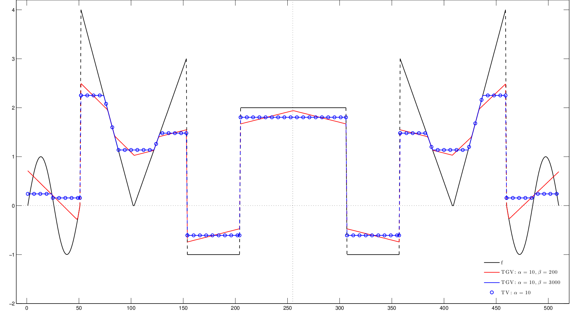
Figure 1. Numerical verification of Theorem 4.10. Using the even function ff shown above as a data function and setting β/α≥L\beta/\alpha\geq L, the solutions of the TGVβ,α2\mathrm{TGV}_{\beta,\alpha}^{2} and α​TV\alpha\,\mathrm{TV} regularisation problems coincide.
Theorem 4.10.

Let f∈BV⁡(−L,L)f\in\mathrm{BV}(-L,L) be an even function. If

(4.15) βα≥L,\frac{\beta}{\alpha}\geq L,

then the solution to the L2L^{2}–TGVβ,α2\mathrm{TGV}_{\beta,\alpha}^{2} regularisation problem is the same with the solution to the following TV\mathrm{TV} regularisation problem:

minu⁡12​∫Ω(u−f)2​𝑑x+α​TV​(u).\min_{u}\;\frac{1}{2}\int_{\Omega}(u-f)^{2}dx+\alpha\,\mathrm{TV}(u).
Proof.

Recall that for every u∈W1,1​(Ω)u\in W^{1,1}(\Omega) the following Poincaré type inequality holds,

‖u−uΩ‖L1​(Ω)≤L​‖∇u‖L1​(Ω),\|u-u_{\Omega}\|_{L^{1}(\Omega)}\leq L\|\nabla u\|_{L^{1}(\Omega)},

where uΩ=1ℒ⁡(Ω)​∫Ωu​𝑑xu_{\Omega}=\frac{1}{\mathcal{L}(\Omega)}\int_{\Omega}u~dx, see for example [AFP00]. Using density arguments, we can prove that the same inequality holds for BV with the same constant, i.e., for every u∈BV⁡(Ω)u\in\mathrm{BV}(\Omega)

(4.16) ‖u−uΩ‖L1​(Ω)≤L​‖D​u‖ℳ.\|u-u_{\Omega}\|_{L^{1}(\Omega)}\leq L\|Du\|_{\mathcal{M}}.

Since ff is even, from Proposition 4.8 we have that the solution of

(4.17) minu∈BV⁡(Ω)⁡12​∫Ω(u−f)2​𝑑x+TGVβ,α2​(u),\min_{u\in\mathrm{BV}(\Omega)}\;\frac{1}{2}\int_{\Omega}(u-f)^{2}dx+\mathrm{TGV}_{\beta,\alpha}^{2}(u),

is an even function as well. Thus, the problem (4.17) is equivalent to

(4.18) minu∈BV⁡(Ω)u​ even⁡12​∫Ω(u−f)2​𝑑x+TGVβ,α2​(u).\min_{\begin{subarray}{c}u\in\mathrm{BV}(\Omega)\\ u\text{ even}\end{subarray}}\;\frac{1}{2}\int_{\Omega}(u-f)^{2}dx+\mathrm{TGV}_{\beta,\alpha}^{2}(u).

Similarly we can prove that the outcome of TV regularisation for even data, is even as well. Thus, it suffices to prove that for an even function uu, we have TGVβ,α2​(u)=α​TV​(u):=α​‖D​u‖ℳ\mathrm{TGV}_{\beta,\alpha}^{2}(u)=\alpha\,\mathrm{TV}(u):=\alpha\|Du\|_{\mathcal{M}}, provided (4.15) holds. We calculate successively:

TGVβ,α2​(u)\displaystyle\mathrm{TGV}_{\beta,\alpha}^{2}(u) =minw∈BV⁡(Ω)⁡α​‖D​u−w‖M+β​‖D​w‖ℳ\displaystyle=\min_{w\in\mathrm{BV}(\Omega)}\;\alpha\|Du-w\|_{M}+\beta\|Dw\|_{\mathcal{M}}
≤α​‖D​u‖ℳ\displaystyle\leq\alpha\|Du\|_{\mathcal{M}} OPEN(choosing ​w=0),\displaystyle\text{(choosing }w=0),
≤α​‖D​u−wΩ‖ℳ\displaystyle\leq\alpha\|Du-w_{\Omega}\|_{\mathcal{M}} ∀w∈BV⁡(Ω),(from Lemma 4.9),\displaystyle\forall w\in\mathrm{BV}(\Omega),(\text{from Lemma \ref{Lemma_even_plus_linear}}),
≤α​‖D​u−w‖ℳ+α​‖w−wΩ‖L1​(Ω)\displaystyle\leq\alpha\|Du-w\|_{\mathcal{M}}+\alpha\|w-w_{\Omega}\|_{L^{1}(\Omega)}
≤α​‖D​u−w‖ℳ+β​α​Lβ​‖D​w‖ℳ\displaystyle\leq\alpha\|Du-w\|_{\mathcal{M}}+\frac{\beta\alpha L}{\beta}\|Dw\|_{\mathcal{M}} (Poincaré inequality),
≤max⁡{1,a​Lβ}​(α​‖D​u−w‖ℳ+β​‖D​w‖ℳ)\displaystyle\leq\max\left\{1,\frac{aL}{\beta}\right\}\left(\alpha\|Du-w\|_{\mathcal{M}}+\beta\|Dw\|_{\mathcal{M}}\right)
=α​‖D​u−w‖ℳ+β​‖D​w‖ℳ\displaystyle=\alpha\|Du-w\|_{\mathcal{M}}+\beta\|Dw\|_{\mathcal{M}} (since (4.15) holds).\displaystyle(\text{since \eqref{a_b_even} holds}).

Finally, we have

α​‖D​u‖ℳ\displaystyle\alpha\|Du\|_{\mathcal{M}} ≤α∥Du−w∥ℳ+β∥Dw∥ℳ∀w∈BV(Ω)⇒\displaystyle\leq\alpha\|Du-w\|_{\mathcal{M}}+\beta\|Dw\|_{\mathcal{M}}\quad\forall w\in\mathrm{BV}(\Omega)\Rightarrow
α​‖D​u‖ℳ\displaystyle\alpha\|Du\|_{\mathcal{M}} ≤minw∈BV⁡(Ω)⁡α​‖D​u−w‖ℳ+β​‖D​w‖ℳ\displaystyle\leq\min_{w\in\mathrm{BV}(\Omega)}\alpha\|Du-w\|_{\mathcal{M}}+\beta\|Dw\|_{\mathcal{M}}
=TGVβ,α2​(u),\displaystyle=\mathrm{TGV}_{\beta,\alpha}^{2}(u),

and the proof is complete. ∎

In Figure 1 we verify numerically the above result. Both TGV and TV minimisation problems are solved with the Chambolle-Pock primal dual method [CP11] as it is described in [Bre12].

5. Computation of exact solutions

In this section we compute exact solutions for the TGVβ,α2\mathrm{TGV}_{\beta,\alpha}^{2} regularisation problem for several data functions ff. In particular we calculate exact solutions for simple piecewise constant, piecewise affine and hat functions. We are focusing on the relation between the structure of solutions and the parameters α\alpha and β\beta.

5.1. Piecewise constant function with a single jump

For convenience in the calculation, for this section, Ω\Omega will be an interval of the form (0,2​L)(0,2L). We define ff to be a piecewise function with a single jump, i.e.,

(5.1) f⁡(x)={0if ​x∈(0,L),hif ​x∈[L,2​L),f(x)=\begin{cases}0&\text{if }\;x\in(0,L),\\ h&\text{if }\;x\in[L,2L),\end{cases}

for some h>0h>0, see Figure 2.

Refer to caption
Figure 2. Piecewise constant function ff with a jump discontinuity at x=Lx=L.

In order to compute exact solutions for ff our strategy is as follows: Firstly, we investigate what are the possible types of solutions, describing them in a qualitative way and secondly we calculate them explicitly.

Since after a simple translation ff is an even function and TGVβ,α2\mathrm{TGV}_{\beta,\alpha}^{2} is translation invariant [BKP09], from Proposition 4.8 we have that the solution uu will be symmetric with respect to the point (L,h/2)(L,h/2). That is to say

(5.2) u⁡(x)=−u⁡(2​L−x)+h,for all ​x∈(L,2​L).u(x)=-u(2L-x)+h,\quad\text{for all }x\in(L,2L).

Thus, we only need to describe the solution in (0,L)(0,L). The following theorem states which kinds of solutions are allowed to occur.

Theorem 5.1.

Let uu be the solution to the L2L^{2}–TGVβ,α2\mathrm{TGV}_{\beta,\alpha}^{2} regularisation problem for the piecewise constant function defined in (5.1). Then uu can only have the following form on (0,L)(0,L):

  • •

    There exists 0<x1<L0<x_{1}<L such that uu is strictly negative and affine in (0,x1)(0,x_{1}) with u⁡(x1)=0u(x_{1})=0.

  • •

    There exists potentially 0<x1≤x~1<L0<x_{1}\leq\tilde{x}_{1}<L such that u=0u=0 in [x1,x~1][x_{1},\tilde{x}_{1}].

  • •

    u>0u>0 in (x~1,L)(\tilde{x}_{1},L) consisting of at most two affine parts of increasing gradient in (x~1,x2)(\tilde{x}_{1},x_{2}) and (x2,L)(x_{2},L) respectively with x~1<x2<L\tilde{x}_{1}<x_{2}<L. Moreover, in the case x~1=x1\tilde{x}_{1}=x_{1}, uu has the same gradient in (0,x1)(0,x_{1}) and (x1,x2)(x_{1},x_{2}).

Note.

In fact, as we will see later, x~1\tilde{x}_{1} must be equal to x1x_{1}, i.e., the allowed solutions will be strictly negative in (0,x1)(0,x_{1}) and strictly positive in (x1,L)(x_{1},L). However this is not obvious by simply interpreting the optimality conditions Cf, Cα and Cβ (which is how Theorem 5.1 is proved) but it is a result of subsequent calculations.

Proof of Theorem 5.1.

Let us note firstly that from Propositions 4.2 and 4.3 we have that uu is continuous on (0,L)(0,L) with u−​(L)≥0u^{-}(L)\geq 0. Also, from Proposition 4.4 we have that if u<0u<0 on a set of the form (0,x1)(0,x_{1}) then uu must be affine there. Moreover Proposition 4.1 implies that there is not an interval (c,d)⊆(0,L)(c,d)\subseteq(0,L) such that u<0u<0 (u>0u>0) on (c,d)(c,d) with u+​(c)=u−​(d)=0u^{+}(c)=u^{-}(d)=0. Indeed, for the negative case, there would be a point x∈(c,d)x\in(c,d) such that uu is affine on (c,x)(c,x) and (x,d)(x,d) with strictly negative and strictly positive gradient respectively on these intervals. But then u′u^{\prime} would be strictly increasing in an interval where u¯<f¯\overline{u}<\underline{f} a contradiction. We work similarly for the positive case. We conclude that uu can be strictly negative only in an interval of the type (0,c)(0,c), 0≤c≤L0\leq c\leq L and strictly positive only in an interval of the type (d,L)(d,L), 0≤d≤L0\leq d\leq L possibly consisting of two affine parts of increasing gradient. In particular uu would be increasing in (0,L)(0,L). The proof will be complete if we prove that the following situations cannot happen:

  1. (i)

    u>0u>0 in (0,L)(0,L).

  2. (ii)

    u=0u=0 in (0,x1)(0,x_{1}), 0<x1<L0<x_{1}<L and u>0u>0 in (x1,L)(x_{1},L).

  3. (iii)

    u=0u=0 in (0,L)(0,L).

  4. (iv)

    u<0u<0 in (0,x1)(0,x_{1}), 0<x1<L0<x_{1}<L and u=0u=0 in x1,Lx_{1},L.

  5. (v)

    u<0u<0 in (0,L)(0,L).

For (i) suppose that u>0u>0 in (0,L)(0,L). By symmetry we would have that u<hu<h in (L,2​L)(L,2L). This means that the dual function vv would be strictly convex in (0,L)(0,L), strictly concave in (L,2​L)(L,2L) with v+​(0)=v′⁣+​(0)=v−​(2​L)=v′⁣−​(2​L)=0v^{+}(0)=v^{\prime+}(0)=v^{-}(2L)=v^{\prime-}(2L)=0 something that cannot happen.

For (ii) suppose that there exists 0<x1<L0<x_{1}<L such that u=0u=0 in (0,x1)(0,x_{1}) and u>0u>0 in (x1,L)(x_{1},L). Then vv will be an affine function in (0,x1)(0,x_{1}) (condition (Cf)) but since v∈H02​(0,2​L)v\in H_{0}^{2}(0,2L) we have that v=0v=0 in (0,x1)(0,x_{1}). Moreover D​u=0Du=0 and thus w=0w=0 a.e. in (0,x1)(0,x_{1}) because otherwise from condition (Cα) we would have that |v′|=α|v^{\prime}|=\alpha on a set of positive measure in (0,x1)(0,x_{1}). Now, since u>0u>0 in (x1,L)(x_{1},L) (assume w.l.o.g. that uu is affine there) from Proposition 4.1 we have that w=D​u=c>0w=Du=c>0 something that forces ww to have a jump discontinuity at x1x_{1} and thus from (Cβ) we get that v⁡(x1)=β>0v(x_{1})=\beta>0. However, this contradicts to the continuity of vv.

For (iii) suppose that u=0u=0 in (0,L)(0,L). Then by symmetry we would have that u=hu=h in (L,2​L)(L,2L). Thus, from condition (Cf) again, vv will be affine in those intervals and again from its boundary conditions and its continuity we get that v=0v=0 on (0,L)(0,L). But since uu has a jump discontinuity at x=Lx=L, according to condition (Cα) we must have v′=−αv^{\prime}=-\alpha, a contradiction.

For (iv) suppose that there exists 0<x1<L0<x_{1}<L such that u<0u<0 in (0,x1)(0,x_{1}) and u=0u=0 in (x1,L)(x_{1},L). Then vv would be strictly convex and thus have a strictly increasing derivative in (0,x1)(0,x_{1}). Since v′⁣+​(0)=0v^{\prime+}(0)=0 we have that v′​(x1)>0v^{\prime}(x_{1})>0. Moreover, vv would be affine in (x1,L)(x_{1},L) with positive gradient equal to v′​(x1)v^{\prime}(x_{1}), something that forces v⁡(L)>0v(L)>0. However, as after a simple translation ff is an odd function, and according to Proposition 4.7 the same will be true for the continuous function vv, then we must have v⁡(L)=0v(L)=0. The case (v) is proved in a similar way.

Finally, for the last statement of the proposition, suppose that u<0u<0 in (0,x1)(0,x_{1}), u>0u>0 in (x1,L)(x_{1},L) and the derivative of uu has a jump discontinuity at x1x_{1}. Since D​u=wDu=w, in (0,x1)(0,x_{1}) and (x1,L)(x_{1},L) we have that ww will have a jump discontinuity at x1x_{1} and condition (Cβ) imposes that |v⁡(x1)|=β|v(x_{1})|=\beta. The case v⁡(x1)=−βv(x_{1})=-\beta is impossible as vv is strictly increasing in (0,x1)(0,x_{1}) and also if v⁡(x1)=βv(x_{1})=\beta, from the fact that v′​(x1)>0v^{\prime}(x_{1})>0 and v′v^{\prime} is continuous as x1x_{1} we have that vv is increasing in (x1,x1+δ)(x_{1},x_{1}+\delta) for some δ>0\delta>0, thus v⁡(x1+δ)>βv(x_{1}+\delta)>\beta, contradicting (Cβ). ∎

Notice how we take advantage of the symmetries of uu and vv in order to prove Theorem 5.1. It remains to rule out the possibility that x1<x~1x_{1}<\tilde{x}_{1}. In particular, we have to show that the four following situations cannot occur 11 1 N: negative, 0: zero, P1: positive one affine part, P2: positive two affine parts, J: jump discontinuity, C: continuous.:

(N-0-P1-J) u<0​ in ​(0,x1),u=0​ in ​(x1,x~1),u>0​ with 1 affine part in ​(x~1,L), jump at ​x=L,\displaystyle u<0\text{ in }(0,x_{1}),\;u=0\text{ in }(x_{1},\tilde{x}_{1}),\;u>0\text{ with 1 affine part in }(\tilde{x}_{1},L),\text{ jump at }x=L,
(N-0-P2-J) u<0​ in ​(0,x1),u=0​ in ​(x1,x~1),u>0​ with 2 affine parts in  in ​(x~1,L), jump at ​x=L,\displaystyle u<0\text{ in }(0,x_{1}),\;u=0\text{ in }(x_{1},\tilde{x}_{1}),\;u>0\text{ with 2 affine parts in }\text{ in }(\tilde{x}_{1},L),\text{ jump at }x=L,
(N-0-P1-C) u<0​ in ​(0,x1),u=0​ in ​(x1,x~1),u>0​ with 1 affine part in ​(x~1,L), continuous at ​x=L,\displaystyle u<0\text{ in }(0,x_{1}),\;u=0\text{ in }(x_{1},\tilde{x}_{1}),\;u>0\text{ with 1 affine part in }(\tilde{x}_{1},L),\text{ continuous at }x=L,
(N-0-P2-C) u<0​ in ​(0,x1),u=0​ in ​(x1,x~1),u>0​ with 2 affine parts in ​(x~1,L), continuous at ​x=L,\displaystyle u<0\text{ in }(0,x_{1}),\;u=0\text{ in }(x_{1},\tilde{x}_{1}),\;u>0\text{ with 2 affine parts in }(\tilde{x}_{1},L),\text{ continuous at }x=L,

where 0<x1<x~1<L0<x_{1}<\tilde{x}_{1}<L. In the following we will only show that for (N-0-P1-J), the proof of the rest three cases is done similarly.

Proposition 5.2.

The case (N-0-P1-J) cannot occur.

Proof.

Suppose that u<0u<0 in (0,x1)(0,x_{1}), u=0u=0 in (x1,x~1)(x_{1},\tilde{x}_{1}) and u>0u>0 and affine in (x~1,L)(\tilde{x}_{1},L) with 0<x1<x~1<L0<x_{1}<\tilde{x}_{1}<L. Then we claim that in that case, u′u^{\prime} is constant, say equal to c>0c>0, in (0,x1)∪(x~1,L)(0,x_{1})\cup(\tilde{x}_{1},L), w=cw=c in (0,L)(0,L) and vv is affine in (x1,x~1)(x_{1},\tilde{x}_{1}) with gradient equal to α\alpha there. Indeed, let cc be the value of the derivative of uu in (0,x1)(0,x_{1}). We know already from Proposition 4.1 that w=u′w=u^{\prime} there. Now, if w≠cw\neq c on a set of positive measure in (x1,x~1)(x_{1},\tilde{x}_{1}), that will mean that D​w≠0Dw\neq 0 somewhere in (x1,x~1)(x_{1},\tilde{x}_{1}) and thus from (Cβ), vv must be ±β\pm\beta somewhere in (x1,x~1)(x_{1},\tilde{x}_{1}). But this is not possible since vv is strictly convex in (0,x1)(0,x_{1}), v′⁣+​(0)=0v^{\prime+}(0)=0, affine in (x1,x~1)(x_{1},\tilde{x}_{1}) and thus vv is strictly increasing in (0,x~1)(0,\tilde{x}_{1}). Moreover, w=v′=cw=v^{\prime}=c in (x~1,L)(\tilde{x}_{1},L) because otherwise ww would have a jump discontinuity on x~1\tilde{x}_{1}, something that forces v⁡(x~1)=βv(\tilde{x}_{1})=\beta but this cannot happen since v′​(x~1)>0v^{\prime}(\tilde{x}_{1})>0. Finally, since D​u−w=−cDu-w=-c in (x1,x~1)(x_{1},\tilde{x}_{1}), from condition (Cα) we have that v′=αv^{\prime}=\alpha there.

Also note that since uu has a jump discontinuity at x=Lx=L, condition (Cα) forces v′​(L)=−αv^{\prime}(L)=-\alpha and from the symmetry of vv we must have v⁡(L)=0v(L)=0.

For convenience we set

ℓ1=x1>0,ℓ2=x~1−x1>0,ℓ3=L−x~1>0with ​ℓ1+ℓ2+ℓ3=L.\ell_{1}=x_{1}>0,\quad\ell_{2}=\tilde{x}_{1}-x_{1}>0,\quad\ell_{3}=L-\tilde{x}_{1}>0\quad\text{with }\ell_{1}+\ell_{2}+\ell_{3}=L.

and

v1=v⌊(0,x1),v2=v⌊(x1,x~1),v3=v⌊(x~1,L).v_{1}=v\lfloor(0,x_{1}),\quad v_{2}=v\lfloor(x_{1},\tilde{x}_{1}),\quad v_{3}=v\lfloor(\tilde{x}_{1},L).

Since uu is an affine function on (0,x1)(0,x_{1}) we have that v1v_{1} is a cubic function

v1​(x)=a1​x3+b1​x2+c1​x+d1,x∈(0,x1),v_{1}(x)=a_{1}x^{3}+b_{1}x^{2}+c_{1}x+d_{1},\quad x\in(0,x_{1}),

that satisfies the conditions

(5.3) v1​(0)=0,v1′​(0)=0,v1′​(ℓ1)=α,v1′′​(ℓ1)=0.v_{1}(0)=0,\quad v_{1}^{\prime}(0)=0,\quad v_{1}^{\prime}(\ell_{1})=\alpha,\quad v_{1}^{\prime\prime}(\ell_{1})=0.

Thus v1v_{1} will have the form

(5.4) v1​(x)=−α3​ℓ12​x3+αℓ1​x2,x∈(0,x1).v_{1}(x)=-\frac{\alpha}{3\ell_{1}^{2}}x^{3}+\frac{\alpha}{\ell_{1}}x^{2},\quad x\in(0,x_{1}).

Since v2v_{2} is an affine function on (x1,x2)(x_{1},x_{2}) with gradient α\alpha and vv is continuous at x1x_{1}, we have that v2v_{2} will be of the form

(5.5) v2​(x)=α⁡(x−ℓ1)+2​α​ℓ13,x∈(x1,x~1).v_{2}(x)=\alpha(x-\ell_{1})+\frac{2\alpha\ell_{1}}{3},\quad x\in(x_{1},\tilde{x}_{1}).

Since uu is a strictly positive affine function on (x~1,L)(\tilde{x}_{1},L) (with the same gradient as in (0,x1)(0,x_{1})), we have that v3v_{3} must be a cubic function

v3​(x)=a3​x3+b3​x2+c3​x+d3,x∈(x~1,L),v_{3}(x)=a_{3}x^{3}+b_{3}x^{2}+c_{3}x+d_{3},\quad x\in(\tilde{x}_{1},L),

that satisfies the following conditions at x=x~1=ℓ1+ℓ2x=\tilde{x}_{1}=\ell_{1}+\ell_{2}:

(5.6) v3​(ℓ1+ℓ2)=α​ℓ2+2​α​ℓ13,v3′​(ℓ1+ℓ2)=α,v3′′​(ℓ1+ℓ2)=0,v3′′′​(ℓ1)​(ℓ1+ℓ2)=−2​αℓ12,v_{3}(\ell_{1}+\ell_{2})=\alpha\ell_{2}+\frac{2\alpha\ell_{1}}{3},\quad v_{3}^{\prime}(\ell_{1}+\ell_{2})=\alpha,\quad v_{3}^{\prime\prime}(\ell_{1}+\ell_{2})=0,\quad v_{3}^{\prime\prime\prime}(\ell_{1})(\ell_{1}+\ell_{2})=-\frac{2\alpha}{\ell_{1}^{2}},

and also the following conditions at x=L=ℓ1+ℓ2+ℓ3x=L=\ell_{1}+\ell_{2}+\ell_{3}:

(5.7) v3​(ℓ1+ℓ2+ℓ3)=0,v_{3}(\ell_{1}+\ell_{2}+\ell_{3})=0,
(5.8) v3′​(ℓ1+ℓ2+ℓ3)=−α.v_{3}^{\prime}(\ell_{1}+\ell_{2}+\ell_{3})=-\alpha.

The conditions (5.6) give

(5.9) v3​(x)=−α3​ℓ12​(x−ℓ1−ℓ2)3+α⁡(x−ℓ1−ℓ2)+α​ℓ2+2​α​ℓ13,x∈(x~1,L).v_{3}(x)=-\frac{\alpha}{3\ell_{1}^{2}}(x-\ell_{1}-\ell_{2})^{3}+\alpha(x-\ell_{1}-\ell_{2})+\alpha\ell_{2}+\frac{2\alpha\ell_{1}}{3},\quad x\in(\tilde{x}_{1},L).

What is left is to find the relationship among ℓ1\ell_{1}, ℓ2\ell_{2} and ℓ3\ell_{3}. Condition (5.8) gives

(5.10) ℓ3=2​ℓ1,\ell_{3}=\sqrt{2}\ell_{1},

and the condition (5.7) together with (5.10) gives

(5.11) 2+23​ℓ1+ℓ2=0,\frac{2+\sqrt{2}}{3}\ell_{1}+\ell_{2}=0,

which is a contradiction since both ℓ1\ell_{1} and ℓ2\ell_{2} are strictly positive. Thus, this kind of solution cannot occur. ∎

From all the previous results, it follows that only the following situations can occur:

(N-P1-J) u⁡<0​ in ​(0,x1),u>​0​ with 1 affine part in ​(x1,L), jump at ​x=L,\displaystyle u<0\text{ in }(0,x_{1}),\;u>0\text{ with 1 affine part in }(x_{1},L),\text{ jump at }x=L,
(N-P2-J) u⁡<0​ in ​(0,x1),u>​0​ with 2 affine parts in ​(x1,L), jump at ​x=L,\displaystyle u<0\text{ in }(0,x_{1}),\;u>0\text{ with 2 affine parts in }(x_{1},L),\text{ jump at }x=L,
(N-P1-C) u⁡<0​ in ​(0,x1),u>​0​ with 1 affine part in ​(x1,L), continuous at ​x=L,\displaystyle u<0\text{ in }(0,x_{1}),\;u>0\text{ with 1 affine part in }(x_{1},L),\text{ continuous at }x=L,
(N-P2-C) u⁡<0​ in ​(0,x1),u>​0​ with 2 affine parts in ​(x1,L), continuous at ​x=L,\displaystyle u<0\text{ in }(0,x_{1}),\;u>0\text{ with 2 affine parts in }(x_{1},L),\text{ continuous at }x=L,

where 0<x1<L0<x_{1}<L.

Refer to caption
(a) Solution of the type
N-P1-J.
Refer to caption
(b) Solution of the type
N-P2-J.
Refer to caption
(c) Solution of the type
N-P1-C.
Refer to caption
(d) Solution of the type
N-P2-C.
Figure 3. All the possible types of solution uu to the minimisation problem ( P ) for the data function ff defined in (5.1). We also show the forms of the corresponding variables ww and vv.

In Figure 3 we provide a qualitative description on how these four allowed solutions look like, along with the corresponding variables ww and vv. Notice that the solution of the type N-P1-C will be in fact the L2L^{2}–linear regression of ff. Our next step is to identify the combinations of the parameters α\alpha and β\beta that lead to each type of solution.

Proposition 5.3 (N-P1-J).

The solution uu of the problem ( P ) with the data function ff defined in (5.1) is of the type N-P1-J, see Figure 3(a), if and only if α\alpha and β\beta satisfy the conditions

(5.12) βα≥4​L27 and α<h​L8.\frac{\beta}{\alpha}\geq\frac{4L}{27}\quad\text{ and }\quad\alpha<\frac{hL}{8}.

More specifically in that case:

(5.13) u={6​αL2x−2​αL,ifx∈(0,L),6​αL2(x−L)+h−4​αL,ifx∈(L,2​L),u=\begin{cases}\frac{6\alpha}{L^{2}}x-\frac{2\alpha}{L},\quad&\text{if}\quad x\in(0,L),\\ \frac{6\alpha}{L^{2}}(x-L)+h-\frac{4\alpha}{L},\quad&\text{if}\quad x\in(L,2L),\end{cases}

i.e., uu has a jump discontinuity of size h−8​α/Lh-8\alpha/L at x=Lx=L.

Proof.

It is easy to check that the solution uu will be of the type N-P1-J if and only if we can find a function vv in [0,L][0,L] that satisfies the following conditions:

(5.14) vv is a cubic polynomial, (from condition (Cf),v′′=−u, is an affine function),\displaystyle(\text{from condition }\eqref{C1},v^{\prime\prime}=-u,\text{ is an affine function}),
(5.15) v⁡(0)=0,v′​(0)=0,\displaystyle v(0)=0,\;v^{\prime}(0)=0,\qquad (boundary conditions for vv),
(5.16) v⁡(L)=0,\displaystyle v(L)=0,\qquad (vv is an odd function),
(5.17) v′​(L)=−α,\displaystyle v^{\prime}(L)=-\alpha,\qquad (u jumps at L, condition (Cα)),\displaystyle(\text{$u$ jumps at $L$, condition \eqref{C2}}),
(5.18) 0<−v′′​(L)<h2,\displaystyle 0<-v^{\prime\prime}(L)<\frac{h}{2},\qquad (u jumps at L & symmetry),\displaystyle(\text{$u$ jumps at $L$ $\&$ symmetry}),
(5.19) |v′|≤α,\displaystyle|v^{\prime}|\leq\alpha,\qquad (condition (Cα)),\displaystyle(\text{condition \eqref{C2}}),
(5.20) |v|≤β,\displaystyle|v|\leq\beta,\qquad (condition (Cβ)).\displaystyle(\text{condition \eqref{C3}}).

It is now easy to check that the function

v⁡(x)=−αL2​x3+αL​x2,x∈[0,L],v(x)=-\frac{\alpha}{L^{2}}x^{3}+\frac{\alpha}{L}x^{2},\quad x\in[0,L],

satisfies conditions (5.14)–(5.17) and also the condition (5.19). Observe that vv obtains it maximum in [0,L][0,L] at x=2​L/3x=2L/3, with v⁡(2​L/3)=4​α​L/27v(2L/3)=4\alpha L/27, thus (5.20) can be written as

4​α​L27≤β.\frac{4\alpha L}{27}\leq\beta.

Finally, condition (5.18) can be written as

0<4​αL<h2.0<\frac{4\alpha}{L}<\frac{h}{2}.

The last two inequalities form the conditions in (5.12). Using the fact that u=−v′′u=-v^{\prime\prime} in (0,L)(0,L) and taking advantage of the symmetry of u, we have (5.13). ∎

We now proceed to the study of the case N-P2-J. As we will see, it is computationally inaccessible to find the exact conditions on α\alpha and β\beta that result to this kind of solution but we are able to provide some sufficient conditions that are not far away from being necessary as well.

Proposition 5.4 (N-P2-J).

If α\alpha and β\beta satisfy the conditions

(5.21) βα​<4​L27 and β>​4​α23​h,\frac{\beta}{\alpha}<\frac{4L}{27}\quad\text{ and }\quad\beta>\frac{4\alpha^{2}}{3h},

then the solution uu of the problem ( P ) with the data function ff defined in (5.1) is of the type N-P2-J, see Figure 3(b). More specifically, there exist points 0<x1<x2<00<x_{1}<x_{2}<0 with

x1=x22 and L−3​βα<x2<L−9​β4​α,x_{1}=\frac{x_{2}}{2}\quad\text{ and }\quad L-\frac{3\beta}{\alpha}<x_{2}<L-\frac{9\beta}{4\alpha},

such that u<0u<0 and u>0u>0 in (0,x1)(0,x_{1}) and (x1,L)(x_{1},L) respectively with u′u^{\prime} having a positive jump at x2x_{2}.

Proof.

Again, it is easily verified that uu will be a solution of the type N-P2-J if and only if we can find ℓ1>0\ell_{1}>0, ℓ2>0\ell_{2}>0 with ℓ1+ℓ2=L\ell_{1}+\ell_{2}=L and two functions v1v_{1}, v2v_{2} defined on [0,ℓ1][0,\ell_{1}] and [ℓ1,ℓ1+ℓ2][\ell_{1},\ell_{1}+\ell_{2}] respectively, such that the following conditions are satisfied:

(5.22) v1, v2 are cubic polynomials,\displaystyle\text{$v_{1}$, $v_{2}$ are cubic polynomials},\qquad (from condition (Cf)),\displaystyle(\text{from condition }\eqref{C1}),
(5.23) v1​(0)=0,v1′​(0)=0,\displaystyle v_{1}(0)=0,\;v_{1}^{\prime}(0)=0,\qquad (boundary conditions for v),\displaystyle(\text{boundary conditions for $v$}),
(5.24) v1​(ℓ1)=β,v1′​(ℓ1)=0,\displaystyle v_{1}(\ell_{1})=\beta,\;v_{1}^{\prime}(\ell_{1})=0,\qquad (v has a maximum at ℓ1, condition (Cα)),\displaystyle(\text{$v$ has a maximum at $\ell_{1}$, condition \eqref{C2}}),
(5.25) v2​(ℓ1)=β,v2′​(ℓ1)=0,v2′′​(ℓ1)=v1′′​(ℓ1),\displaystyle v_{2}(\ell_{1})=\beta,\;v_{2}^{\prime}(\ell_{1})=0,\;v_{2}^{\prime\prime}(\ell_{1})=v_{1}^{\prime\prime}(\ell_{1}),\qquad (continuity of v, v′ and u),\displaystyle(\text{continuity of $v$, $v^{\prime}$ and u}),
(5.26) v2′′′​(ℓ1)<v1′′′​(ℓ1),\displaystyle v_{2}^{\prime\prime\prime}(\ell_{1})<v_{1}^{\prime\prime\prime}(\ell_{1}),\qquad (u′u^{\prime} has a positive jump at ℓ1\ell_{1})
(5.27) v2​(L)=0,\displaystyle v_{2}(L)=0,\qquad (vv is an odd function),
(5.28) v2′​(L)=−α,\displaystyle v_{2}^{\prime}(L)=-\alpha,\qquad (u jumps at L, condition (Cα)),\displaystyle(\text{$u$ jumps at $L$, condition \eqref{C2}}),
(5.29) 0<−v2′′​(L)<h2,\displaystyle 0<-v_{2}^{\prime\prime}(L)<\frac{h}{2},\qquad (u jumps at L & symmetry),\displaystyle(\text{$u$ jumps at $L$ $\&$ symmetry}),
(5.30) |vi′|≤α,i=1,2,\displaystyle|v_{i}^{\prime}|\leq\alpha,\;i=1,2,\qquad (condition (Cα)),\displaystyle(\text{condition \eqref{C2}}),
(5.31) |vi|≤β,i=1,2,\displaystyle|v_{i}|\leq\beta,\;i=1,2,\qquad (condition (Cβ)).\displaystyle(\text{condition \eqref{C3}}).

From conditions (5.22)–(5.24), we get that

(5.32) v1​(x)=−2​βℓ13​x3+3​βℓ12​x2,x∈[0,ℓ1].v_{1}(x)=-\frac{2\beta}{\ell_{1}^{3}}x^{3}+\frac{3\beta}{\ell_{1}^{2}}x^{2},\quad x\in[0,\ell_{1}].

We can also check that condition (5.30) for v2v_{2} is equivalent to

(5.33) 3​β2​α≤ℓ1,\frac{3\beta}{2\alpha}\leq\ell_{1},

while condition (5.31) is satisfied. After some computations, we have that conditions (5.25), (5.27), (5.28) give that v2v_{2} will be of the form

(5.34) v2​(x)=(2​βℓ12​ℓ2−α3​ℓ22)​(x−ℓ1)3−3​βℓ12​(x−ℓ1)2+β.v_{2}(x)=\left(\frac{2\beta}{\ell_{1}^{2}\ell_{2}}-\frac{\alpha}{3\ell_{2}^{2}}\right)(x-\ell_{1})^{3}-\frac{3\beta}{\ell_{1}^{2}}(x-\ell_{1})^{2}+\beta.

We also get the following relationship between ℓ1\ell_{1} and ℓ2\ell_{2}:

(5.35) γ​ℓ22+ℓ2​ℓ12−γ​ℓ12=0, with γ:=3​βα,\gamma\ell_{2}^{2}+\ell_{2}\ell_{1}^{2}-\gamma\ell_{1}^{2}=0,\quad\text{ with }\quad\gamma:=\frac{3\beta}{\alpha},

where one can check that ℓ2<γ\ell_{2}<\gamma independently of the value of ℓ1\ell_{1}. Notice now, that if the condition (5.26) is satisfied, then v2v_{2} will be decreasing, with decreasing derivative as well something that would imply that conditions (5.30)–(5.31) hold for v2v_{2}. With the help of (5.34), (5.35) and condition ℓ1+ℓ2=L\ell_{1}+\ell_{2}=L, we get that condition (5.26) is equivalent to

(5.36) ℓ12−2​L​ℓ1+2​γ​L<0.\ell_{1}^{2}-2L\ell_{1}+2\gamma L<0.

The inequality (5.36) is true if and only if

(5.37) γ<L2andL−L2−2​γ​L<ℓ1⇔ℓ2<L2−2​γ​L.\gamma<\frac{L}{2}\quad\text{and}\quad L-\sqrt{L^{2}-2\gamma L}<\ell_{1}\iff\ell_{2}<\sqrt{L^{2}-2\gamma L}.

From the fact that ℓ1+ℓ2=L\ell_{1}+\ell_{2}=L and (5.35) we get that ℓ2\ell_{2} is the unique solution of

(5.38) ϕ⁡(ℓ2):=γ​ℓ22γ−ℓ2+ℓ2−L=0.\phi(\ell_{2}):=\sqrt{\frac{\gamma\ell_{2}^{2}}{\gamma-\ell_{2}}}+\ell_{2}-L=0.

In view of (5.38) we have that ℓ2=L2−2​γ​L\ell_{2}=\sqrt{L^{2}-2\gamma L} if and only if γ=4​L/9\gamma=4L/9. Since ϕ\phi is strictly increasing, one can check that (5.37) is equivalent to the very simple expression

(5.39) βα<4​L27.\frac{\beta}{\alpha}<\frac{4L}{27}.

Notice that in that case (5.33) is also satisfied. Finally, the last condition that has to be satisfied is (5.29). Using (5.34) and (5.35) it can be checked that it is equivalent to

(5.40) 4​ℓ2−2​γℓ22<h2​α.\frac{4\ell_{2}-2\gamma}{\ell_{2}^{2}}<\frac{h}{2\alpha}.

Ideally, one would like to obtain an explicit expression for ℓ2\ell_{2} from (5.38) and obtain an inequality involving α\alpha and β\beta using (5.40). However, this is practically impossible as one would have to solve a cubic equation for ℓ2\ell_{2}. This is why we are giving some estimates instead. One can check that from (5.38) and (5.39) we can derive that

(5.41) 34​γ<ℓ2<γ.\frac{3}{4}\gamma<\ell_{2}<\gamma.

We have that the expression (4​ℓ2−2​γ)/ℓ22(4\ell_{2}-2\gamma)/\ell_{2}^{2} in (5.40) is a strictly increasing function of ℓ2\ell_{2} provided that ℓ2<γ\ell_{2}<\gamma which is true in our case. Thus, in order to satisfy (5.40) a sufficient (but not necessary) condition is

4​γ−2​γγ2<h2​α⇔β>4​α23​h.\frac{4\gamma-2\gamma}{\gamma^{2}}<\frac{h}{2\alpha}\iff\beta>\frac{4\alpha^{2}}{3h}.

∎

Remark.

Let us also point out the following fact: Suppose that α∗\alpha^{\ast} and β∗\beta^{\ast} are such, so that conditions (5.21) hold, i.e., the solution is of the type N-P2-J. Then there exists a 0<c<β∗0<c<\beta^{\ast} such that for every β≤c\beta\leq c the condition (5.40) is violated, so we do not have this type of solution. Indeed from (5.40) and (5.41) we have that

169​γ<4​ℓ2−2​γℓ22<h2​α.\frac{16}{9\gamma}<\frac{4\ell_{2}-2\gamma}{\ell_{2}^{2}}<\frac{h}{2\alpha}.

Thus keeping α\alpha fixed and choosing β\beta such that

(5.42) 16γ>h2​α⇔β<32​α227​h\frac{16}{\gamma}>\frac{h}{2\alpha}\iff\beta<\frac{32\alpha^{2}}{27h}

we cannot have the solution of the type N-P2-J any more.

We now turn our attention to the solution of the type N-P1-C. As we mentioned earlier, in that case uu is an affine function and thus also the L2L^{2}–linear regression of ff. In Theorem 4.5 we gave some thresholds for α\alpha and β\beta in the general case but we can be more explicit in this specific example.

Proposition 5.5 (N-P1-C).

The solution uu of the problem ( P ) with the data function defined in (5.1) is of the type N-P1-C, see Figure 3(c), if and only if α\alpha and β\beta satisfy the conditions

(5.43) α≥h​L8 and β≥h​L254.\alpha\geq\frac{hL}{8}\quad\text{ and }\quad\beta\geq\frac{hL^{2}}{54}.

Moreover, in that case uu will be the L2L^{2}–linear regression of ff and equal to

(5.44) u⁡(x)=3​h4​L​x−h4,x∈(0,2​L).u(x)=\frac{3h}{4L}x-\frac{h}{4},\quad x\in(0,2L).
Proof.

Again we can check that the solution will be of the type N-P1-C if and only if we can find a function vv defined on [0,L][0,L] such that the following conditions hold:

(5.45) v is a cubic polynomial,\displaystyle\text{$v$ is a cubic polynomial},\qquad
(5.46) v⁡(0)=0,v′​(0)=0,\displaystyle v(0)=0,\;v^{\prime}(0)=0,\qquad
(5.47) v⁡(L)=0,\displaystyle v(L)=0,\qquad
(5.48) −v′′​(L)=h2,\displaystyle-v^{\prime\prime}(L)=\frac{h}{2},\qquad (condition (Cf), continuity at L & symmetry),\displaystyle\text{(condition \eqref{C1}, continuity at L \& symmetry)},
(5.49) |v′|≤α,\displaystyle|v^{\prime}|\leq\alpha,\qquad
(5.50) |v|≤β.\displaystyle|v|\leq\beta.\qquad

We can easily check that conditions (5.45)–(5.48) give

(5.51) v⁡(x)=−h8​L​x3+h8​x2,x∈[0,L].v(x)=-\frac{h}{8L}x^{3}+\frac{h}{8}x^{2},\quad x\in[0,L].

Moreover, the maximum values of |v||v| and |v′||v^{\prime}| are h​L254\frac{hL^{2}}{54} and h​L8\frac{hL}{8} respectively. Thus, conditions (5.49)–(5.50) will be satisfied if and only if (5.43) holds. ∎

Finally, we investigate under which combinations of α\alpha and β\beta we have solutions of the type N-P2-C. As in the case N-P2-J, it is computationally inaccessible to provide exact conditions, thus we provide again some sufficient but not necessary conditions.

Proposition 5.6 (N-P2-C).

If α\alpha and β\beta satisfy the conditions

(5.52) β<h​L254 and ​β≤4​L​α9−L227,\beta<\frac{hL^{2}}{54}\quad\text{ and }\beta\leq\frac{4L\alpha}{9}-\frac{L^{2}}{27},

then the solution uu of the problem ( P ) with the data function ff defined in (5.1) is of the type N-P2-C, see Figure 3(d), and u′u^{\prime} has a positive jump at a point x2x_{2} where 2​L3<x2<L\frac{2L}{3}<x_{2}<L.

Proof.

As in the N-P2-J case, uu will be a solution of the type N-P2-C if and only if we can find ℓ1>0\ell_{1}>0, ℓ2>0\ell_{2}>0 with ℓ1+ℓ2=L\ell_{1}+\ell_{2}=L and two functions defined on [0,ℓ1][0,\ell_{1}] and [ℓ1,ℓ1+ℓ2][\ell_{1},\ell_{1}+\ell_{2}] respectively, such that the following conditions are satisfied:

(5.53) v1, v2 are cubic polynomials,\displaystyle\text{$v_{1}$, $v_{2}$ are cubic polynomials},\qquad
(5.54) v1​(0)=0,v1′​(0)=0,\displaystyle v_{1}(0)=0,\;v_{1}^{\prime}(0)=0,\qquad
(5.55) v1​(ℓ1)=β,v1′​(ℓ1)=0,\displaystyle v_{1}(\ell_{1})=\beta,\;v_{1}^{\prime}(\ell_{1})=0,\qquad
(5.56) v2​(ℓ1)=β,v2′​(ℓ1)=0,v2′′​(ℓ1)=v1′′​(ℓ1),\displaystyle v_{2}(\ell_{1})=\beta,\;v_{2}^{\prime}(\ell_{1})=0,\;v_{2}^{\prime\prime}(\ell_{1})=v_{1}^{\prime\prime}(\ell_{1}),\qquad
(5.57) v2′′′​(ℓ1)<v1′′′​(ℓ1),\displaystyle v_{2}^{\prime\prime\prime}(\ell_{1})<v_{1}^{\prime\prime\prime}(\ell_{1}),\qquad
(5.58) v2​(L)=0,\displaystyle v_{2}(L)=0,\qquad
(5.59) −v′′​(L)=h2,\displaystyle-v^{\prime\prime}(L)=\frac{h}{2},\qquad (condition (Cf), continuity at L & symmetry),\displaystyle\text{(condition \eqref{C1}, continuity at L \& symmetry)},
(5.60) |vi′|≤α,i=1,2,\displaystyle|v_{i}^{\prime}|\leq\alpha,\;i=1,2,\qquad
(5.61) |vi|≤β,i=1,2.\displaystyle|v_{i}|\leq\beta,\;i=1,2.\qquad

Conditions (5.53)–(5.55) together with (5.60)–(5.61) yield

(5.62) v1​(x)=−2​βℓ13​x3+3​βℓ12​x2,x∈[0,ℓ1],v_{1}(x)=-\frac{2\beta}{\ell_{1}^{3}}x^{3}+\frac{3\beta}{\ell_{1}^{2}}x^{2},\quad x\in[0,\ell_{1}],

with

(5.63) 3​β2​α≤ℓ1.\frac{3\beta}{2\alpha}\leq\ell_{1}.

Supposing that v2v_{2} is of the form

v2​(x)=a3​(x−ℓ1)3+a2​(x−ℓ1)2+a1​(x−ℓ1)+a0,x∈[ℓ1,ℓ1+ℓ2],v_{2}(x)=a_{3}(x-\ell_{1})^{3}+a_{2}(x-\ell_{1})^{2}+a_{1}(x-\ell_{1})+a_{0},\quad x\in[\ell_{1},\ell_{1}+\ell_{2}],

conditions (5.56), (5.58), (5.59) give

(5.64) v2​(x)=a3​(x−ℓ1)3−3​βℓ12​(x−ℓ1)2+β,x∈[ℓ1,ℓ1+ℓ2],v_{2}(x)=a_{3}(x-\ell_{1})^{3}-\frac{3\beta}{\ell_{1}^{2}}(x-\ell_{1})^{2}+\beta,\quad x\in[\ell_{1},\ell_{1}+\ell_{2}],
(5.65) a3​ℓ23−3​β​ℓ22ℓ12+β\displaystyle a_{3}\ell_{2}^{3}-\frac{3\beta\ell_{2}^{2}}{\ell_{1}^{2}}+\beta =\displaystyle= 0,\displaystyle 0,
(5.66) −6​a3​ℓ2+6​βℓ12\displaystyle-6a_{3}\ell_{2}+\frac{6\beta}{\ell_{1}^{2}} =\displaystyle= h2.\displaystyle\frac{h}{2}.

One can check that conditions (5.56) and (5.59) impose v2′v_{2}^{\prime} to be decreasing , so in order to satisfy (5.60) and (5.61) it suffices to impose |v2′​(ℓ1+ℓ2)|≤α|v_{2}^{\prime}(\ell_{1}+\ell_{2})|\leq\alpha, which, with the help of (5.64) and (5.66), is equivalent to

(5.67) 3​β​ℓ2ℓ12+h​ℓ24≤α.\frac{3\beta\ell_{2}}{\ell_{1}^{2}}+\frac{h\ell_{2}}{4}\leq\alpha.

Moreover combining (5.65), (5.66) and the fact that ℓ1+ℓ2=L\ell_{1}+\ell_{2}=L, we can get a relationship between ℓ1\ell_{1} and ℓ1\ell_{1} and an equation for ℓ2\ell_{2}:

(5.68) ℓ2=12​βh+24​βℓ12,\ell_{2}=\sqrt{\frac{12\beta}{h+\frac{24\beta}{\ell_{1}^{2}}}},
(5.69) ϕ⁡(ℓ1):=ℓ1+12​βh+24​βℓ12−L=0.\phi(\ell_{1}):=\ell_{1}+\sqrt{\frac{12\beta}{h+\frac{24\beta}{\ell_{1}^{2}}}}-L=0.

It is easy to see that the equation (5.69) has a unique solution in (0,L)(0,L) but one has to solve a quartic in order to express it explicitly. Thus, as in the case N-P2-J we give some estimates. Observe firstly that using (5.62), (5.64), (5.66) and (5.68) condition (5.57) is satisfied if and only if

(5.70) 18​β​ℓ1ℓ2−6​β​ℓ13ℓ23<−12​β,\frac{18\beta\ell_{1}}{\ell_{2}}-\frac{6\beta\ell_{1}^{3}}{\ell_{2}^{3}}<-12\beta,

which is satisfied if and only if ℓ2<ℓ12\ell_{2}<\frac{\ell_{1}}{2}. However, from (5.68), this is true if and only if ℓ1>24​βh\ell_{1}>\sqrt{\frac{24\beta}{h}}. From the fact that the function ϕ\phi is strictly increasing, the last inequality is true if and only if

(5.71) β<h​L254.\beta<\frac{hL^{2}}{54}.

It remains to identify some sufficient conditions for (5.67). Observe that under (5.71) we have ϕ⁡(2​L/3)<0\phi(2L/3)<0 and ϕ⁡(L>0)\phi(L>0), which means that

(5.72) 2​L3<ℓ1<L and 0<ℓ2<L3.\frac{2L}{3}<\ell_{1}<L\quad\text{ and }\quad 0<\ell_{2}<\frac{L}{3}.

Using (5.72), we find that a sufficient (but not necessary) condition for (5.67) is

(5.73) 3​β(2​L3)2​L3+h​L12<α⇔β≤4​L​α9−L2​h27.\frac{3\beta}{(\frac{2L}{3})^{2}}\frac{L}{3}+\frac{hL}{12}<\alpha\iff\beta\leq\frac{4L\alpha}{9}-\frac{L^{2}h}{27}.

We can easily verify that under (5.73) the condition (5.63) is satisfied as well. ∎

Refer to caption
Figure 4. Illustration of the four different types of solutions of ( P ) for the piecewise constant function ff that result for different combinations of the parameters α\alpha and β\beta.

We now summarise how the solutions of the problem ( P ) with the data function ff are affected by the different choices of the parameters α\alpha and β\beta. In Figure 4 we have partitioned the set {α>0,β>0}\{\alpha>0,\;\beta>0\} into different areas that correspond to the four different possible solutions. These areas are:

  1. (1)

    Blue colour: {α<h​L8,β≥4​L27​α}\left\{\alpha<\frac{hL}{8},\;\beta\geq\frac{4L}{27}\alpha\right\}, (necessary and sufficient condition), N-P1-J, see Figure 3(a).

  2. (2)

    Purple colour: {β<4​L27​α,β≥3627​h​α2}\left\{\beta<\frac{4L}{27}\alpha,\;\beta\geq\frac{36}{27h}\alpha^{2}\right\}, (sufficient condition), N-P2-J, see Figure 3(b).

  3. (3)

    Yellow colour: {α≥h​L8,β≥h​L254}\left\{\alpha\geq\frac{hL}{8},\;\beta\geq\frac{hL^{2}}{54}\right\}, (necessary and sufficient condition), N-P1-C, see Figure 3(c).

  4. (4)

    Orange colour: {β≤3227​h​α2,β<h​L254}\left\{\beta\leq\frac{32}{27h}\alpha^{2},\;\beta<\frac{hL^{2}}{54}\right\}, (sufficient condition), N-P2-C, see Figure 3(d).

Notice that according to Proposition 5.6 our initial sufficient conditions for the solution of the type N-P2-C to happen were β<h​L254\beta<\frac{hL^{2}}{54} and β≤4​L9​α−L2​h27\beta\leq\frac{4L}{9}\alpha-\frac{L^{2}h}{27}. However, according to the Remark after Proposition 5.4 when condition β≤3227​h​α2\beta\leq\frac{32}{27h}\alpha^{2} holds then the solution of the type N-P2-J cannot happen and since the conditions for N-P1-C and N-P2-C are necessary and sufficient we conclude that when β≤3227​h​α2\beta\leq\frac{32}{27h}\alpha^{2} holds (together with α≤h​L8\alpha\leq\frac{hL}{8}) then the solution of the type N-P2-C occur. Notice that

{α>0,β>0:β≤4​L9α−L2​h27,α≤h​L8}⊆{α>0,β>0:β≤3227​hα2,α≤h​L8},\{\alpha>0,\;\beta>0:\;\beta\leq\frac{4L}{9}\alpha-\frac{L^{2}h}{27},\;\alpha\leq\frac{hL}{8}\}\subseteq\{\alpha>0,\;\beta>0:\;\beta\leq\frac{32}{27h}\alpha^{2},\;\alpha\leq\frac{hL}{8}\},

see Figure 4.

As we mentioned, due to computational issues it is difficult to derive necessary and sufficient conditions for the solutions of the type N-P2-J and N-P2-C. However, the estimates we have provided are not far away from being sharp as the unknown grey area in Figure 4, {β>3227​h​α2,β<3627​h​α2,β<4​L27​α}\{\beta>\frac{32}{27h}\alpha^{2},\;\beta<\frac{36}{27h}\alpha^{2},\;\beta<\frac{4L}{27}\alpha\} is relatively small.

5.2. Piecewise affine function with a single jump

In this section we are choosing the data function to be a simple piecewise affine function gg, see Figure 5. However, as we will see, we do not have to perform the previous computations to identify solutions for ( P ) as the solutions have a close connection with the ones that correspond to the piecewise constant function ff.

Refer to caption
Figure 5. The piecewise affine function gg. It has a jump discontinuity at x=Lx=L and the gradient in the affine parts is equal to λ\lambda.
Proposition 5.7.

Let ff and gg be the following functions on (0,2​L)(0,2L):

f⁡(x)={0 if ​x∈(0,L),h if ​x∈(L,2​L),g⁡(x)={λ⁡(x−L)if ​x∈(0,L),λ⁡(x−L)+hif ​x∈(L,2​L).f(x)=\begin{cases}0&\text{ if }\;\;\;x\in(0,L),\\ h&\text{ if }\;\;\;x\in(L,2L),\end{cases}\qquad\ g(x)=\begin{cases}\lambda(x-L)&\text{if }\;x\in(0,L),\\ \lambda(x-L)+h&\text{if }\;x\in(L,2L).\end{cases}

Then ufu_{f} is a solution to the minimisation problem P with data function ff if and only if ugu_{g} is a solution with data function gg, where

ug​(x)=uf​(x)+λ⁡(x−L).u_{g}(x)=u_{f}(x)+\lambda(x-L).
Proof.

Suppose that ufu_{f} is a solution of ( P ) with data ff, for some combination of the parameters α\alpha and β\beta and let vfv_{f}, wfw_{f} to be the corresponding dual variables. We will show that ug​(x)=uf​(x)+λ⁡(x−L)u_{g}(x)=u_{f}(x)+\lambda(x-L) is a solution for data gg for the same combination of α\alpha and β\beta and vice versa. The optimality conditions (Cf), (Cα), (Cβ) read:

vf′′\displaystyle v_{f}^{\prime\prime} =\displaystyle= f−uf,\displaystyle f-u_{f},
−vf\displaystyle-v_{f} ∈\displaystyle\in α​Sgn​(D​uf−wf),\displaystyle\alpha\,\mathrm{Sgn}(Du_{f}-w_{f}),
vf\displaystyle v_{f} ∈\displaystyle\in β​Sgn​(D​wf).\displaystyle\beta\,\mathrm{Sgn}(Dw_{f}).

Observing that we have g⁡(x)=f⁡(x)+λ⁡(x−L)g(x)=f(x)+\lambda(x-L) we set vg=vfv_{g}=v_{f} and wg​(x)=wf​(x)+λw_{g}(x)=w_{f}(x)+\lambda. Then we have

vg′′=vf′′=f−uf=g−ug,\displaystyle v_{g}^{\prime\prime}=v_{f}^{\prime\prime}=f-u_{f}=g-u_{g},
−vg′∈α​Sgn​(D​ug−wg)⇔−vg′∈α​Sgn​(D​uf+λ−wf−λ)⇔−vf′∈α​Sgn​(D​uf−wf),\displaystyle-v^{\prime}_{g}\in\alpha\,\mathrm{Sgn}(Du_{g}-w_{g})\iff-v^{\prime}_{g}\in\alpha\,\mathrm{Sgn}(Du_{f}+\lambda-w_{f}-\lambda)\iff-v^{\prime}_{f}\in\alpha\,\mathrm{Sgn}(Du_{f}-w_{f}),

and also

vg∈β​Sgn​(D​wg)⇔vg∈β​Sgn​(D​wf)⇔vf∈β​Sgn​(D​wf),\displaystyle v_{g}\in\beta\,\mathrm{Sgn}(Dw_{g})\iff v_{g}\in\beta\,\mathrm{Sgn}(Dw_{f})\iff v_{f}\in\beta\,\mathrm{Sgn}(Dw_{f}),

thus (Cf), (Cα), (Cβ) hold for ugu_{g}, vgv_{g} and wgw_{g}. Similarly, we show that if ugu_{g} is a solution for data gg then uf​(x):=ug​(x)−λ⁡(x−L)u_{f}(x):=u_{g}(x)-\lambda(x-L) is a solution for data ff.

∎

Refer to caption
(a) Solution of the type
N-P1-J.
Refer to caption
(b) Solution of the type
N-P2-J.
Refer to caption
(c) Solution of the type
N-P1-C.
Refer to caption
(d) Solution of the type
N-P2-C.
Figure 6. All the possible types of solution uu to the minimisation problem P for the data function gg.

In Figure 6 we show all such possible solutions. These solutions correspond to the same combinations of α\alpha and β\beta that are shown in Figure 4. One can observe here the capability of TGV to preserve piecewise affine structures. This is in contrast to TV regularisation which promotes piecewise constant reconstructions.

5.3. Hat function
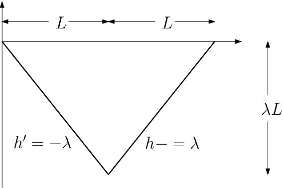
Refer to caption
Figure 7. The hat function h.

In this section we are computing exact solutions for the hat function

(5.74) h⁡(x)=λ​|x−L|−λ​L,x∈(0,2​L),h(x)=\lambda|x-L|-\lambda L,\quad x\in(0,2L),

where λ>0\lambda>0, see Figure 7. The study of this case gives an insight about how TGV deals with local extrema. Note again that the solutions will be symmetric, as hh is as well. Working similarly as we did for the function ff, we conclude that the only possible types of solutions uu are the following:

(C-E-C) uu is constant on (0,x1)(0,x_{1}), equal to hh on (x1,x2)(x_{1},x_{2}) and constant on (x1,L)(x_{1},L), where (0<x1<x2<L)(0<x_{1}<x_{2}<L),
(A-E-A) uu is affine on (0,x1)(0,x_{1}), equal to hh on (x1,x2)(x_{1},x_{2}), and affine on (x1,L)(x_{1},L), where (0<x1<x2<L)(0<x_{1}<x_{2}<L),
(C) uu is constant on (0,L)(0,L),
(A) uu is affine on (0,L)(0,L),
Refer to caption
(a) Solution of the type C-E-C
Refer to caption
(b) Solution of the type A-E-A
Refer to caption
(c) Solution of the type C
Refer to caption
(d) Solution of the type A
Figure 8. All the possible types of solution uu to the minimisation problem ( P ) for the data function hh defined in (5.74). We also show the forms of the corresponding variables ww and vv.

In Figure 8 we show how these four types of solutions look like along with the corresponding variables ww and vv. Notice that the solution of the type C is the L2L^{2}–linear regression. Also, the solution of the type C-E-C corresponds to the TV–like solutions predicted by Theorem 4.10. In the following, we investigate which combinations of the parameters α\alpha and β\beta correspond to each solution. Unlike the case with the piecewise constant function ff, we are able to give necessary and sufficient conditions for every case.

Proposition 5.8.

Let hh be the hat function defined in (5.74). Then the solution uu of the problem ( P ) can be of the following type:

  1. (1)

    The solution uu is of the type C-E-C, Figure 8(a), if and only if

    (5.75) α<λ​L28 and β≥α​L−2​α3​2​αλ.\alpha<\frac{\lambda L^{2}}{8}\quad\text{ and }\quad\beta\geq\alpha L-\frac{2\alpha}{3}\sqrt{\frac{2\alpha}{\lambda}}.

    In that case

    u⁡(x)={−2​α​λif ​x∈(0,2​αλ),−λ​xif ​x∈(2​αλ,L−2​αλ),−λ​L+2​α​λOPENif ​x∈(L−2​αλ),L).u(x)=\begin{cases}-\sqrt{2\alpha\lambda}&\text{if }\;x\in\left(0,\sqrt{\frac{2\alpha}{\lambda}}\right),\\ -\lambda x&\text{if }\;x\in\left(\sqrt{\frac{2\alpha}{\lambda}},L-\sqrt{\frac{2\alpha}{\lambda}}\right),\\ -\lambda L+\sqrt{2\alpha\lambda}&\text{if }\;x\in\left(L-\sqrt{\frac{2\alpha}{\lambda}}),L\right).\end{cases}
  2. (2)

    The solution uu is of the type A-E-A, Figure 8(b), if and only if

    (5.76) β>2​L​α3 and β<α​L−2​α3​2​αλ.\beta>\frac{2L\alpha}{3}\quad\text{ and }\quad\beta<\alpha L-\frac{2\alpha}{3}\sqrt{\frac{2\alpha}{\lambda}}.

    In that case

    u⁡(x)={−μ​x−2​α​(λ−μ)if ​x∈(0,32​(L−βα)),−λ​xif ​x∈(32​(L−βα),L−32​(L−βα)),−μ​x−(λ−μ)​L+2​2​α​(λ−μ)if ​x∈(L−32​(L−βα),L),​ with ​μ=λ−8​α9​(L−βα)2.u(x)=\begin{cases}-\mu x-\sqrt{2\alpha(\lambda-\mu)}&\text{if }\;x\in\left(0,\frac{3}{2}\left(L-\frac{\beta}{\alpha}\right)\right),\\ -\lambda x&\text{if }\;x\in\left(\frac{3}{2}\left(L-\frac{\beta}{\alpha}\right),L-\frac{3}{2}\left(L-\frac{\beta}{\alpha}\right)\right),\\ -\mu x-(\lambda-\mu)L+2\sqrt{2\alpha(\lambda-\mu)}&\text{if }\;x\in\left(L-\frac{3}{2}\left(L-\frac{\beta}{\alpha}\right),L\right),\end{cases}\;\text{ with }\;\mu=\lambda-\frac{8\alpha}{9\left(L-\frac{\beta}{\alpha}\right)^{2}}.
  3. (3)

    The solution uu is of the type C, Figure 8(c), if and only if

    (5.77) β≥λ​L312 and α≥λ​L28.\beta\geq\frac{\lambda L^{3}}{12}\quad\text{ and }\quad\alpha\geq\frac{\lambda L^{2}}{8}.

    In that case

    u⁡(x)=λ​L2,x∈(0,2​L).u(x)=\frac{\lambda L}{2},\quad x\in(0,2L).
  4. (4)

    The solution uu is of the type A, Figure 8(d), if and only if

    (5.78) β<λ​L312 and β≤2​L​α3.\beta<\frac{\lambda L^{3}}{12}\quad\text{ and }\quad\beta\leq\frac{2L\alpha}{3}.

    In that case

    u⁡(x)=μ|x−L|−(λ​L−t), with μ=λ−12​βL3 and t=6​βL2.u(x)=\mu|x-L|-(\lambda L-t),\quad\text{ with }\quad\mu=\lambda-\frac{12\beta}{L^{3}}\quad\text{ and }\quad t=\frac{6\beta}{L^{2}}.
Proof.

(1) Since we are looking at solutions of the type C-E-C, we must find 0<x1<x2<L0<x_{1}<x_{2}<L such that u=tu=t for a constant tt on (0,x1)(0,x_{1}), u=hu=h on (x1,x2)(x_{1},x_{2}) and u=−t−λ⁡(x2−x1)u=-t-\lambda(x_{2}-x_{1}) on (x2,L)(x_{2},L). As far as the variable ww is concerned, we have that w=D​u=0w=Du=0 on (0,x1)∪(x2,L)(0,x_{1})\cup(x_{2},L). However since u=fu=f on (x1,x2)(x_{1},x_{2}), we have that vv is affine in that interval, thus it cannot have an extremum there. Thus, condition (Cβ) forces w=0w=0 on (x1,x2)(x_{1},x_{2}) as well and (Cα) forces v′=αv^{\prime}=\alpha there. We conclude that the solution uu will be of the type C-E-C if and only if we can find 0<x1<x2<L0<x_{1}<x_{2}<L and a function vv with the following properties:

(5.79) v and v′ are continuous,\displaystyle\text{$v$ and $v^{\prime}$ are continuous},\qquad (v∈H02),\displaystyle\text{($v\in H_{0}^{2}$)},
(5.80) v is a cubic polynomial on (0,x1) and (x2,L),\displaystyle\text{$v$ is a cubic polynomial on $(0,x_{1})$ and $(x_{2},L)$},\qquad (condition (Cf)),\displaystyle\text{(condition \eqref{C1})},
(5.81) v⁡(0)=0,v′​(0)=0,\displaystyle v(0)=0,\;v^{\prime}(0)=0,\qquad (boundary conditions for v),\displaystyle\text{(boundary conditions for $v$)},
(5.82) v is affine and v′=α on (x1,x2),\displaystyle\text{$v$ is affine and $v^{\prime}=\alpha$ on $(x_{1},x_{2})$},\qquad (as explained above),\displaystyle(\text{as explained above}),
(5.83) v′​(L)=0,\displaystyle v^{\prime}(L)=0,\qquad (v is an even function),\displaystyle\text{($v$ is an even function)},
(5.84) |v|≤β,\displaystyle|v|\leq\beta,\qquad (condition (Cβ)),\displaystyle\text{(condition \eqref{C3})},
(5.85) |v′|≤α,\displaystyle|v^{\prime}|\leq\alpha,\qquad (condition (Cα)).\displaystyle\text{(condition \eqref{C2})}.

After some computations we find that

x1=L−x2=2​αλ,t=2​α​λ,x_{1}=L-x_{2}=\sqrt{\frac{2\alpha}{\lambda}},\quad t=\sqrt{2\alpha\lambda},
v⁡(x)={−λ6​x3+α​λ2​x2if ​x∈(0,2​αλ),α⁡(x−x1)+λ​x123if ​x∈(2​αλ,L−2​αλ),−λ6​(x+x1−L)3+α⁡(x+x1−L)+α⁡(L−2​x1)+λ​x133if ​x∈(L−2​αλ,L).v(x)=\begin{cases}-\frac{\lambda}{6}x^{3}+\sqrt{\frac{\alpha\lambda}{2}}x^{2}&\text{if }\;x\in\left(0,\sqrt{\frac{2\alpha}{\lambda}}\right),\\ \alpha(x-x_{1})+\frac{\lambda x_{1}^{2}}{3}&\text{if }\;x\in\left(\sqrt{\frac{2\alpha}{\lambda}},L-\sqrt{\frac{2\alpha}{\lambda}}\right),\\ -\frac{\lambda}{6}(x+x_{1}-L)^{3}+\alpha(x+x_{1}-L)+\alpha(L-2x_{1})+\frac{\lambda x_{1}^{3}}{3}&\text{if }\;x\in\left(L-\sqrt{\frac{2\alpha}{\lambda}},L\right).\end{cases}

From the equation v′′=h−uv^{\prime\prime}=h-u we can get an expression for uu. Moreover x1<x2x_{1}<x_{2} holds if and only if

α<λ​L28.\alpha<\frac{\lambda L^{2}}{8}.

Finally one catch check that (5.85) holds and since vv is increasing on (0,L)(0,L), in order to satisfy (5.84), it suffices to have v⁡(L)≤βv(L)\leq\beta something that translates to

β≥α​L−2​α3​2​αλ.\beta\geq\alpha L-\frac{2\alpha}{3}\sqrt{\frac{2\alpha}{\lambda}}.

(2) The proof follows essentially the proof of (1)(1). Here we are looking for solutions of the type u=−μ​x−tu=-\mu x-t instead of u=tu=t on (0,x1)(0,x_{1}). In addition to the conditions (5.79)–(5.85) for vv here we also have

(5.86) v⁡(L)=β,(condition (Cβ)),v(L)=\beta,\qquad\text{(condition \eqref{C3})},

because ww makes a positive jump at x=Lx=L, see also Figure 8(b). Again after some computations we find

x1=L−x2=2​αλ−μ,t=2​α​(λ−μ),x_{1}=L-x_{2}=\sqrt{\frac{2\alpha}{\lambda-\mu}},\quad t=\sqrt{2\alpha(\lambda-\mu)},
v⁡(x)={−λ−μ6​x3+α⁡(λ−μ)2​x2if ​x∈(0,2​αλ−μ),α⁡(x−x1)+(λ−μ)​x123if ​x∈(2​αλ−μ,L−2​αλ−μ),−λ−μ6​(x+x1−L)3+α⁡(x+x1−L)+α⁡(L−2​x1)+(λ−μ)​x133if ​x∈(L−2​αλ−μ,L).v(x)=\begin{cases}-\frac{\lambda-\mu}{6}x^{3}+\sqrt{\frac{\alpha(\lambda-\mu)}{2}}x^{2}&\text{if }\;x\in\left(0,\sqrt{\frac{2\alpha}{\lambda-\mu}}\right),\\ \alpha(x-x_{1})+\frac{(\lambda-\mu)x_{1}^{2}}{3}&\text{if }\;x\in\left(\sqrt{\frac{2\alpha}{\lambda-\mu}},L-\sqrt{\frac{2\alpha}{\lambda-\mu}}\right),\\ -\frac{\lambda-\mu}{6}(x+x_{1}-L)^{3}+\alpha(x+x_{1}-L)+\alpha(L-2x_{1})+\frac{(\lambda-\mu)x_{1}^{3}}{3}&\text{if }\;x\in\left(L-\sqrt{\frac{2\alpha}{\lambda-\mu}},L\right).\end{cases}

Again one can check that |v′|<α|v^{\prime}|<\alpha. Moreover the condition v⁡(L)=βv(L)=\beta gives

(5.87) α​L−2​α3​2​αλ−−μ=β⇔μ=λ−8​α9​(L−βα)2.\alpha L-\frac{2\alpha}{3}\sqrt{\frac{2\alpha}{\lambda--\mu}}=\beta\iff\mu=\lambda-\frac{8\alpha}{9\left(L-\frac{\beta}{\alpha}\right)^{2}}.

Since we are looking into cases where 0<μ<λ0<\mu<\lambda we must have 2​αλ−μ>2​αλ\sqrt{\frac{2\alpha}{\lambda-\mu}}>\sqrt{\frac{2\alpha}{\lambda}} and using (5.87) this translates to

(5.88) β<α​L−2​α3​2​αλ.\beta<\alpha L-\frac{2\alpha}{3}\sqrt{\frac{2\alpha}{\lambda}}.

Finally, it is easily checked that in order to impose x1<x2x_{1}<x_{2}, we must have

(5.89) β>2​L​α3.\beta>\frac{2L\alpha}{3}.

(3) In this case, we are looking for solutions of the type u=−tu=-t, t>0t>0. The function vv will be a cubic polynomial that satisfy the conditions:

v⁡(0)=0,v′​(0)=0,v′​(L)=0,v′′=h+t,|v|≤β,|v′|≤α.v(0)=0,\;v^{\prime}(0)=0,\;v^{\prime}(L)=0,\;v^{\prime\prime}=h+t,\;|v|\leq\beta,\;|v^{\prime}|\leq\alpha.

and we easily compute

t=λ​L2,v⁡(x)=−λ6​x3+12​t​x2,x∈(0,L).t=\frac{\lambda L}{2},\quad v(x)=-\frac{\lambda}{6}x^{3}+\frac{1}{2}tx^{2},\quad x\in(0,L).

We can also check that the conditions |v|≤β|v|\leq\beta, |v′|≤α|v^{\prime}|\leq\alpha are equivalent to

β≥λ​L312,α≥λ​L28,\beta\geq\frac{\lambda L^{3}}{12},\quad\alpha\geq\frac{\lambda L^{2}}{8},

respectively.

(4) The proof is similar to (3). We are looking for a solution of the type u⁡(x)=−μ​x−tu(x)=-\mu x-t, x∈(0,L)x\in(0,L), 0<μ<λ0<\mu<\lambda and t>0t>0. As before, the function vv will be a cubic polynomial satisfying the conditions:

v⁡(0)=0,v′​(0)=0,v⁡(L)=β,v′​(L)=0,v′′=h+t,|v|≤β,|v′|≤α.v(0)=0,\;v^{\prime}(0)=0,\;v(L)=\beta,\;v^{\prime}(L)=0,\;v^{\prime\prime}=h+t,\;|v|\leq\beta,\;|v^{\prime}|\leq\alpha.

We get that

v(x)=−λ−μ6x3+t2x2,x∈(0,L),witht=6​βL2,μ=λ−12​βL3.v(x)=-\frac{\lambda-\mu}{6}x^{3}+\frac{t}{2}x^{2},\quad x\in(0,L),\quad\text{with}\quad t=\frac{6\beta}{L^{2}},\quad\mu=\lambda-\frac{12\beta}{L^{3}}.

Thus 0<μ<λ0<\mu<\lambda is equivalent to

β<λ​L312.\beta<\frac{\lambda L^{3}}{12}.

Finally, we check easily that |v|≤β|v|\leq\beta holds and |v′|≤α|v^{\prime}|\leq\alpha is equivalent to

β≤2​L​α3.\beta\leq\frac{2L\alpha}{3}.

∎

Refer to caption
Figure 9. Illustration of the four different types of solutions of ( P ) for the hat function hh that result for different combinations of the parameters α\alpha and β\beta.

As we did for the case of function ff we summarise how the solutions of the problem ( P ) with the data function hh are affected by α\alpha and β\beta. In Figure 9 we have partitioned again the set {α>0,β>0}\{\alpha>0,\;\beta>0\} into different areas that correspond to the four different possible solutions. We note again that in contrast to the cases of the functions ff and gg, here we provide necessary and sufficient conditions for all the four different types of solutions. The corresponding areas are:

  1. (1)

    Blue colour: {α<λ​L28,β≥α​L−2​α3​2​αλ}\left\{\alpha<\frac{\lambda L^{2}}{8},\;\beta\geq\alpha L-\frac{2\alpha}{3}\sqrt{\frac{2\alpha}{\lambda}}\right\}, C-E-C, see Figure 8(a).

  2. (2)

    Purple colour: {β>2​L​α3,β<α​L−2​α3​2​αλ}\left\{\beta>\frac{2L\alpha}{3},\;\beta<\alpha L-\frac{2\alpha}{3}\sqrt{\frac{2\alpha}{\lambda}}\right\}, A-E-A, see Figure 8(b).

  3. (3)

    Yellow colour: {α≥λ​L28,β≥λ​L312}\left\{\alpha\geq\frac{\lambda L^{2}}{8},\;\beta\geq\frac{\lambda L^{3}}{12}\right\}, C, see Figure 8(c).

  4. (4)

    Orange colour: {β<λ​L312,β≤2​L​α3}\left\{\beta<\frac{\lambda L^{3}}{12},\;\beta\leq\frac{2L\alpha}{3}\right\}, A, see Figure 8(d).

6. Numerical experiments

In this final section, we compare our theoretical results with numerical ones obtained by solving the discrete version of ( P ) with the primal-dual algorithm of Chambolle-Pock, [CP11]. A description of the algorithm for TGV minimisation can be found in [Bre12]. We also compute some numerical results with the presence of Gaussian noise that show that TGV regularisation is quite robust in the presence of noise. Let us note here that even though some sensitivity analysis can be done [BV11], it is not an easy task to prove that the corresponding solutions of ( P ) with clean and corrupted data have the same structure provided the noise is sufficiently small. Some relevant work has been done in [BB12] in terms of ground states of regularisation functionals.

In Figure 10, we plot the exact and the numerical solutions of ( P ) using the function ff as a data function. We chose the parameters α\alpha and β\beta so that we have the solution of the type N-P1-J. We observe that for clean data, the exact and the numerical solutions coincide, see Figure 10(a). Moreover, even with the presence of noise, the numerical solution is not far away from the corresponding solution without the noise, Figure 10(b).

We observe similar results in Figures 11 and 12 where we chose the parameters so that we have the solution of the type N-P2-J and N-P1-C respectively.

In Figure 13 we use the hat function hh as a data function. Again, without the presence of noise, the exact solution agrees with the numerical one, Figure 13(a). However, when noise is added, even though the numerical solution is close to the one that corresponds to the clean data, some staircasing is observed, Figure 13(b). This is not surprising as with these combinations of α\alpha and β\beta, TGV behaves like TV as it was shown in Theorem 4.10.

In Figure 14 the parameters are chosen so that the solution of the type A-E-A occurs. In the clean data case we have agreement between the exact and the numerical solution, Figure 14(a), but in the noisy case a kind of “affine” staircasing effect appears in the area where the exact solution equals with the data, see detail of Figure 14(b).

Finally, in Figure 15, the parameters are chosen so the solution of the type A occurs. The numerical solution agrees with the exact one and deviates from it slightly in the presence of noise.

Refer to caption
(a) Clean data, the numerical solution agrees with the exact one.
Refer to caption
(b) Noisy data, the numerical solution deviates slightly from the corresponding exact solution with clean data.
Figure 10. Piecewise constant function ff. The parameters α\alpha and β\beta satisfy the conditions (5.12), thus the solution is of the type N-P1-J.
Refer to caption
(a) Clean data, the numerical solution agrees with the exact one.
Refer to caption
(b) Noisy data, the numerical solution deviates slightly from the corresponding exact solution with clean data.
Figure 11. Piecewise constant function ff. The parameters α\alpha and β\beta satisfy the conditions (5.21), thus the solution is of the type N-P2-J.
Refer to caption
(a) Clean data, the numerical solution agrees with the exact one.
Refer to caption
(b) Noisy data, the numerical solution deviates slightly from the corresponding exact solution with clean data.
Figure 12. Piecewise constant function ff. The parameters α\alpha and β\beta satisfy the conditions (5.43), thus the solution is of the type N-P1-C (L2L^{2}–linear regression).
Refer to caption
(a) Clean data, the numerical solution agrees with the exact one.
Refer to caption
(b) Noisy data, appearance of staircasing effect.
Figure 13. Hat function hh. The parameters α\alpha and β\beta satisfy the conditions (5.75), thus the solution is of the type C-E-C.
Refer to caption
(a) Clean data, the numerical solution agrees with the exact one.
Refer to caption
(b) Noisy data, appearance of an “affine” staircasing effect.
Figure 14. Hat function hh. The parameters α\alpha and β\beta satisfy the conditions (5.76), thus the solution is of the type A-E-A.
Refer to caption
(a) Clean data, the numerical solution agrees with the exact one.
Refer to caption
(b) Noisy data, the numerical solution deviates slightly from the corresponding exact solution with clean data.
Figure 15. Hat function hh. The parameters α\alpha and β\beta satisfy the conditions (5.78), thus the solution is of the type A.

7. Conclusion

We studied exact solutions to the one dimensional L2L^{2}–TGVβ,α2\mathrm{TGV}_{\beta,\alpha}^{2} problem for simple piecewise constant, piecewise affine and hat functions as data terms. We used Fenchel–Rockafellar duality to derive the optimality conditions of the corresponding minimisation problem and we computed the exact solutions using these conditions. The relationship between the values of the parameters α\alpha, β\beta and the structure of solutions was investigated. We performed numerical experiments in which the exact solutions agree with the numerical ones and having only a slight deviation when noise is added.

As far as further research is concerned, the analysis of the exact solutions of the corresponding 2D model should be the first priority as well as a more rigorous study of the problem under the presence of noise.

Acknowledgements

The first author acknowledge the support of the UK Engineering and Physical Sciences Research Council (EPSRC) grant EP/H023348/1 for the University of Cambridge Centre for Doctoral Training, the Cambridge Centre for Analysis, the financial support provided by the EPSRC first grant Nr. EP/J009539/1 “Sparse & Higher-order Image Restoration” and the Award No. KUK-I1-007-43, made by King Abdullah University of Science and Technology (KAUST).

References

  • [AB86] H. Attouch and H. Brezis, Duality for the sum of convex functions in general Banach spaces, North-Holland Mathematical Library 34 (1986), 125–133.
  • [AFP00] L. Ambrosio, N. Fusco, and D. Pallara, Functions of bounded variation and free discontinuity problems, Oxford University Press, USA, 2000.
  • [BB12] Martin Benning and Martin Burger, Ground states and singular vectors of convex variational regularization methods, arXiv preprint arXiv:1211.2057 (2012).
  • [BBBM13] Martin Benning, Christoph Brune, Martin Burger, and Jahn Müller, Higher-order TV methods – Enhancement via Bregman iteration, Journal of Scientific Computing 54 (2013), no. 2-3, 269–310.
  • [BH12] K. Bredies and M. Holler, Artifact-free JPEG decompression with total generalized variation, VISAP 2012: Proceedings of the International Conference on Computer Vision and Applications, 2012.
  • [BKP09] K. Bredies, K. Kunisch, and T. Pock, Total generalized variation, SIAM Journal on Imaging Sciences 3 (2009), 1–42.
  • [BKV13] Kristian Bredies, Karl Kunisch, and Tuomo Valkonen, Properties of L1-TGV2 : The one-dimensional case, Journal of Mathematical Analysis and Applications 398 (2013), no. 1, 438 – 454.
  • [Bre12] K. Bredies, Recovering piecewise smooth multichannel images by minimization of convex functionals with total generalized variation penalty, Preprint (2012).
  • [BV11] K. Bredies and T. Valkonen, Inverse problems with second-order total generalized variation constraints, Proceedings of SampTA 2011 - 9th International Conference on Sampling Theory and Applications, Singapore, 2011.
  • [CCN07] Vicent Caselles, Antonin Chambolle, and Matteo Novaga, The discontinuity set of solutions of the TV denoising problem and some extensions, Multiscale modeling & simulation 6 (2007), no. 3, 879–894.
  • [CE05] T.F. Chan and S. Esedoglu, Aspects of total variation regularized L1{L}^{1} function approximation, SIAM Journal on Applied Mathematics (2005), 1817–1837.
  • [CL97] A. Chambolle and P.L. Lions, Image recovery via total variation minimization and related problems, Numerische Mathematik 76 (1997), 167–188.
  • [CP11] A. Chambolle and T. Pock, A first-order primal-dual algorithm for convex problems with applications to imaging, Journal of Mathematical Imaging and Vision 40 (2011), no. 1, 120–145.
  • [DAG09] V. Duval, J.F. Aujol, and Y. Gousseau, The TVL​1{L1} model: a geometric point of view, SIAM journal on multiscale modeling and simulation 8 (2009), no. 1, 154–189.
  • [DMFLM09] G. Dal Maso, I. Fonseca, G. Leoni, and M. Morini, A higher order model for image restoration: the one dimensional case, SIAM J. Math. Anal 40 (2009), no. 6, 2351–2391.
  • [ET76] I. Ekeland and R. Temam, Convex analysis and variational problems, vol. 1, North Holland, 1976.
  • [Eva10] L.C. Evans, Partial Differential Equations, volume 19 of Graduate Studies in Mathematics, Second Edition, American Mathematical Society,, 2010.
  • [Gra07] M. Grasmair, The equivalence of the taut string algorithm and BV-regularization, Journal of Mathematical Imaging and Vision 27 (2007), no. 1, 59–66.
  • [HHK+03] Walter Hinterberger, Michael Hintermüller, Karl Kunisch, Markus Von Oehsen, and Otmar Scherzer, Tube methods for BV regularization, Journal of Mathematical Imaging and Vision 19 (2003), no. 3, 219–235.
  • [KBPS11] F. Knoll, K. Bredies, T. Pock, and R. Stollberger, Second order total generalized variation (TGV) for MRI, Magnetic Resonance in Medicine 65 (2011), no. 2, 480–491.
  • [Mey01] Yves Meyer, Oscillating patterns in image processing and nonlinear evolution equations: the fifteenth Dean Jacqueline B. Lewis memorial lectures, vol. 22, Amer. Mathematical Society, 2001.
  • [Nik02] Mila Nikolova, Minimizers of cost-functions involving nonsmooth data-fidelity terms. Application to the processing of outliers, SIAM Journal on Numerical Analysis 40 (2002), no. 3, 965–994.
  • [PS08] Christiane Pöschl and Otmar Scherzer, Characterization of minimizers of convex regularization functionals, Contemporary mathematics 451 (2008), 219–248.
  • [PS13] by same author, Exact solutions of one-dimensional TGV, preprint (2013).
  • [Rin00] Wolfgang Ring, Structural properties of solutions to total variation regularization problems, ESAIM: Mathematical Modelling and Numerical Analysis 34 (2000), no. 04, 799–810.
  • [ROF92] L.I. Rudin, S. Osher, and E. Fatemi, Nonlinear total variation based noise removal algorithms, Physica D: Nonlinear Phenomena 60 (1992), no. 1-4, 259–268.
  • [SC03] David Strong and Tony Chan, Edge-preserving and scale-dependent properties of total variation regularization, Inverse problems 19 (2003), no. 6, S165.
  • [Tem85] Roger Temam, Mathematical problems in plasticity, vol. 15, Gauthier-Villars Paris, 1985.
  • [VBK13] T. Valkonen, K. Bredies, and F. Knoll, Total generalized variation in diffusion tensor imaging, SIAM Journal on Imaging Sciences 6 (2013), no. 1, 487–525.