跳到论文正文
W Papers独立论文阅读器 arXiv:1309.5824 论文正文 计算阅读时间 · 0%
引用这篇论文根据当前论文元数据生成,正式投稿前建议核对。


License: arXiv.org perpetual non-exclusive license
arXiv:1309.5824v3 [cond-mat.str-el] 14 Feb 2014

Polaron dynamics and decoherence in an interacting two-spin system coupled to optical phonon environment

Amit Dey1 Affiliation: 1TCMP Div., Saha Institute of Nuclear Physics, Kolkata, India    Sudhakar Yarlagadda1,2 Affiliation: 1TCMP Div., Saha Institute of Nuclear Physics, Kolkata, India Affiliation: 2Cavendish Lab, Univ. of Cambridge, Cambridge, UK
August 24, 2026
Abstract

We study two anisotropically interacting spins coupled to optical phonons; we restrict our analysis to the regime of strong coupling to the environment, to the antiadiabatic region, and to the subspace with zero value for STzS^{z}_{T} (the z-component of the total spin). In the case where each spin is coupled to a different phonon bath, we assume that the system and the environment are initially uncorrelated (and form a simply separable state) in the polaronic frame of reference. By analyzing the polaron dynamics through non-Markovian quantum master equation, we find that the system manifests a small amount of decoherence that decreases both with increasing non-adiabaticity and with enhancing strength of coupling; whereas, under the Markovian approximation, the polaronic system exhibits a decoherence free behavior. For the situation where both spins are coupled to the same phonon bath, we also show that the system is decoherence free in the subspace where STzS^{z}_{T} is fixed. To suppress decoherence through quantum control, we employ a train of pi pulses and demonstrate that unitary evolution of the system can be retained.We propose realization of a weakly decohering charge qubit from an electron in an oxide-based (tunnel-coupled) double quantum dot system.

pacs
71.38.-k, 03.65.Yz, 03.67.Pp

I Introduction

Quantum computation relies on the very quantum features of systems, namely, entanglement and quantum superposition. Due to the ubiquitous presence of system-environment interactions, the quantum coherence is degraded; on total destruction of the quantum superposition, classicality emerges.

The protection of quantum states against decoherence due to interaction with the environment is essential to the development of quantum computational architecture. In this regard quantum robustness strategies have been developed that are passive [such as decoherence free subspaces (DFS)] as well as active [such as quantum Zeno effect (QZE) and its variants]. A DFS is a subspace that is both invariant under the action of the system Hamiltonian and also is spanned by degenerate eigenvectors of the system operators coupling to the environment [1, 2, 3]. QZE is the arresting of decoherence in a quantum system through continuous measurements [4, 5, 6]. Continuous measurement can be approximately achieved if one makes a series of instantaneous measurements with the time interval between consecutive ones being sufficiently small. Mathematically reminiscent of the QZE is the dynamical decoupling through bang-bang control [7, 8, 9]. Now, in this connection, one can think of suppressing the nonunitary evolution of an open system by using an external fast driving field. Earlier, strategies have been proposed to suppress decoherence by perturbing the system (with perturbation being experimentally controllable) in such a manner that the environment can not follow the change of system states anymore; this means, if the perturbation acts on the system much faster than the environmental response time, the system can be effectively decoupled from the environmental fluctuations and thus decoherence is diminished [10, 11].

Using control techniques, achievement of long coherence times has been reported in GaAs and silicon based double quantum dots where the qubit information is encoded in singlet-triplet states involving two spins [12, 13, 14, 15, 16]. Moreover, the two-spin states with fixed z component of the total spin (STz=0S^{z}_{T}=0) are immune to collective decoherence and using Heisenberg exchange interaction universal quantum computation has been proposed for this subspace [17].

In this paper, we consider an anisotropic Heisenberg interaction between two spins with zero value for STzS^{z}_{T}. Each spin is taken to interact strongly with its individual optical phonon bath. For studying the dynamics and decoherence, the polaronic (Lang-Firsov [18] transformed) frame of reference is chosen with polaronic (dressed) basis used for input and output [19]; unlike the interaction in the original frame of reference, the interaction term is weak in the transformed polaronic frame enabling one to carry out perturbation theory. Since both preparation and measurement can be done in the dressed basis, we analyze decoherence in the transformed polaronic frame of reference; thus we seek the possibility of maintaining quantum information encoded in dressed spin (polaron) basis. We study the dynamics of the reduced spin system using quantum master equation approach when initially the system and the environment form a simply separable state. We find that the off-diagonal matrix elements indicate small decoherence under non-Markovian dynamics; on the other hand, Markovian quantum master equation yields decoherence free behavior. We also show that decoherence (in the non-Markovian case) can be suppressed using bang-bang control and unitary evolution of the spin states can be achieved.

For the case where both the spins interact with the same phonon environment (through a global coupling), the system is decoherence free only in the subspace where STzS^{z}_{T} is a fixed constant.

One can produce new oxide-based devices by exploiting their tunability, rich physics, and coupling between the various degrees of freedom (such as charge, lattice, spin, etc.). Here, we also propose that oxide-based double quantum dots with only one electron (tunneling between the dots) can be regarded as a qubit with little decoherence. Strong coupling between electrons and phonons occurs quite commonly in transition metal oxides such as manganites [20, 21, 22]. Oxides, due to the smaller extent of the wavefunction, present a promising alternative to silicon for meeting the demands of miniaturization.

II Model for local phonon coupling

Here we consider the model given by

H\displaystyle H =\displaystyle= Hs+HB+HI,\displaystyle H_{s}+H_{B}+H_{I},

where HsH_{s} is the system Hamiltonian describing the anisotropic Heisenberg interaction between two spins

Hs=J∥S1zS2z−J⟂(S1xS2x+S1yS2y),\displaystyle H_{s}=J_{\lVert}S_{1}^{z}S_{2}^{z}{{-}}J_{\perp}(S_{1}^{x}S_{2}^{x}+S_{1}^{y}S_{2}^{y}), (1)

HBH_{B} corresponds to the phononic bath

HB=ω​∑i=1,2ai†​ai,\displaystyle H_{B}=\omega\sum_{i=1,2}a_{i}^{\dagger}a_{i}, (2)

and HIH_{I} represents the local (i.e., on site) spin-bath interaction

HI=g​ω​∑i=1,2Siz​(ai+ai†).\displaystyle H_{I}=g\omega\sum_{i=1,2}S_{i}^{z}(a_{i}+a_{i}^{\dagger}). (3)

In the above equation, ω\omega is the optical phonon frequency, gg is the spin-phonon coupling parameter (with g2≫1g^{2}\gg 1), and aia_{i} is the phonon destruction operator at site ii. As mentioned in Ref. 23, for manganites 6<g2<106<g^{2}<10. The actual bath and interaction terms involve various momentum modes and have the form HB=∑i,kωk​ai,k†​ai,kH_{B}=\sum_{i,k}\omega_{k}a_{i,k}^{\dagger}a_{i,k} and ∑i,kgk​ωk​Siz​(ai,k+ai,k†)\sum_{i,k}g_{k}\omega_{k}S_{i}^{z}(a_{i,k}+a_{i,k}^{\dagger}) respectively. Initially, for simplicity, we ignore the wavenumber dependence of the coupling and the frequency and take gk=gg_{k}=g and ωk=ω\omega_{k}=\omega; the more general case, involving wavenumber dependence, will be analyzed later in Appendix C. Furthermore, the unperturbed Hamiltonian H0H_{0} is given by

H0=Hs+HB.H_{0}=H_{s}+H_{B}. (4)

Here we are dealing with S=12S=\frac{1}{2} system; consequently, the four eigenstates of HsH_{s} are the triplet states { |↑↑⟩,|↓↓⟩,12(|↑↓⟩+|↓↑⟩)|\uparrow\uparrow\rangle,|\downarrow\downarrow\rangle,\frac{1}{\surd 2}(|\uparrow\downarrow\rangle+|\downarrow\uparrow\rangle)} and the singlet state {12(|↑↓⟩−|↓↑⟩)\frac{1}{\surd 2}(|\uparrow\downarrow\rangle-|\downarrow\uparrow\rangle)}.

III Lang-Firsov transformation

In the non-adiabatic (J⟂ω≤1\frac{J_{\perp}}{\omega}\leq 1) and the strong coupling (g2≫1g^{2}\gg 1) regimes, we make use of the well-known Lang-Firsov (LL) transformation given by [18]

HL=eS​H​e−S,H^{L}=e^{S}He^{-S}, (5)

where S=−∑igSiz(ai−ai†)S=-\sum_{i}gS^{z}_{i}(a_{i}-a_{i}^{\dagger}). Therefore the total Hamiltonian in the Lang-Firsov frame is written as

HL\displaystyle H^{L} =\displaystyle= J∥S1zS2z−J⟂​e−g22(S1+S2−+S2+S1−)\displaystyle J_{\lVert}S_{1}^{z}S_{2}^{z}{{-}}\frac{J_{\perp}e^{-g^{2}}}{2}(S_{1}^{+}S_{2}^{-}+S_{2}^{+}S_{1}^{-}) (6)
+ω∑i=1,2ai†ai−12[J⟂+S1+S2−+J⟂−S2+S1−],\displaystyle+\omega\sum_{i=1,2}a_{i}^{\dagger}a_{i}{{-}}\frac{1}{2}[J_{\perp}^{+}S_{1}^{+}S_{2}^{-}+J_{\perp}^{-}S_{2}^{+}S_{1}^{-}],

where

J⟂±\displaystyle J_{\perp}^{\pm} =\displaystyle= J⟂​e±g⁡[(a2−a2†)−(a1−a1†)]−J⟂​e−g2,\displaystyle J_{\perp}e^{\pm g[(a_{2}-a_{2}^{\dagger})-(a_{1}-a_{1}^{\dagger})]}-J_{\perp}e^{-g^{2}}, (7)

and

J⟂​e−g2\displaystyle J_{\perp}e^{-g^{2}} =\displaystyle= ⟨J⟂​e±g⁡[(a2−a2†)−(a1−a1†)]⟩T=0,\displaystyle\langle J_{\perp}e^{\pm g[(a_{2}-a_{2}^{\dagger})-(a_{1}-a_{1}^{\dagger})]}\rangle_{T=0}, (8)

where the average is taken over the phonon ground state. In the Lang-Firsov frame, we recognize that

HsL=J∥S1zS2z−J⟂​e−g22(S1+S2−+S2+S1−),H_{s}^{L}=J_{\lVert}S_{1}^{z}S_{2}^{z}{{-}}\frac{J_{\perp}e^{-g^{2}}}{2}(S_{1}^{+}S_{2}^{-}+S_{2}^{+}S_{1}^{-}), (9)

as the system Hamiltonian and this describes spins coupled to the same mean phonon field; it is interesting to note that both HsH_{s} and HsLH_{s}^{L} have the singlet as the excited state and the STz=0S^{z}_{T}=0 triplet state as the ground state. Furthermore, as will be shown later, the effective Hamiltonian (obtained from Schrieffer-Wolff transformation, i.e., second-order perturbation theory involving averaging over the ground state of phonons [24, 25]) also has the same ground state and excited state as HsLH_{s}^{L} [see Eq. (37)].

Now, for HsLH_{s}^{L}, in the strong coupling (g2≫1g^{2}\gg 1) and the non-adiabatic (J⟂ω≤1\frac{J_{\perp}}{\omega}\leq 1) regimes the energy difference between the singlet and the STz=0S^{z}_{T}=0 triplet state is J⟂​e−g2≪ωJ_{\perp}e^{-g^{2}}\ll\omega. The interaction Hamiltonian HILH_{I}^{L}, describing the spins coupled to the local phonon fluctuations around the mean field, is given by

HIL\displaystyle H_{I}^{L} =\displaystyle= −12​[J⟂+​S1+​S2−+J⟂−​S2+​S1−],\displaystyle{{-}}\frac{1}{2}[J_{\perp}^{+}S_{1}^{+}S_{2}^{-}+J_{\perp}^{-}S_{2}^{+}S_{1}^{-}], (10)

whereas the environment Hamiltonian HBLH_{B}^{L}, consisting of displaced harmonic oscillators, is expressed as

HBL\displaystyle H_{B}^{L} =\displaystyle= ω​∑i=1,2ai†​ai.\displaystyle\omega\sum_{i=1,2}a_{i}^{\dagger}a_{i}. (11)

Furthermore, the unperturbed Hamiltonian H0LH_{0}^{L} is identified as

H0L=HsL+HBL.\displaystyle H_{0}^{L}=H_{s}^{L}+H_{B}^{L}. (12)

Here, it should be mentioned that the mean field term HsLH_{s}^{L} involves controlled degrees of freedom and hence produces unitary evolution for the system; whereas the interaction Hamiltonian HILH_{I}^{L} contains numerous or uncontrolled environmental degrees of freedom and consequently has the potential for producing decoherence. Now, at this stage, we like to analyze decoherence due to these local environmental fluctuations from a dynamical perspective.

IV Dynamical analysis for local coupling

The two-spin system is exposed to the environment (with which it interacts) thereby making it an open system; we would like to know the reduced system dynamics for this open system. Here, we deal with non-Markovian master equation and try to obtain the off-diagonal elements of the reduced density matrix for the system defined by ρs​(t)≡T​rB​[ρT​(t)]\rho_{s}(t)\equiv Tr_{B}\left[\rho_{T}(t)\right] where the bath degrees of freedom are traced out from the total system-environment density matrix ρT​(t)\rho_{T}(t); the decay of the off-diagonal elements of ρs​(t)\rho_{s}(t) signifies quantum decoherence. We assume that the initial total density matrix is simply separable, i.e., ρT​(0)=ρs​(0)⊗B0\rho_{T}(0)=\rho_{s}(0)\otimes B_{0}, where B0=∑n1,n2|n1,n2⟩p​h⟨n1,n2|e−β​ωn1,n2/Zp​hB_{0}=\sum_{n_{1},n_{2}}|n_{1},n_{2}\rangle_{ph}~\!{}_{ph}\langle n_{1},n_{2}|e^{-\beta\omega_{n_{1},n_{2}}}/Z is the initial thermal density matrix of the bath under thermodynamic equilibrium. The state |n1,n2⟩p​h|n_{1},n_{2}\rangle_{ph} represents a phonon state with n1n_{1} and n2n_{2} being the phonon occupation numbers at sites 11 and 22; furthermore, HBL|n1,n2⟩p​h=ωn1,n2|n1,n2⟩p​h=(n1+n2)ω|n1,n2⟩p​hH_{B}^{L}|n_{1},n_{2}\rangle_{ph}=\omega_{n_{1},n_{2}}|n_{1},n_{2}\rangle_{ph}=(n_{1}+n_{2})\omega|n_{1},n_{2}\rangle_{ph} and ZZ is the partition function for the environment. From here on we use |n⟩p​h≡|n1,n2⟩p​h|n\rangle_{ph}\equiv|n_{1},n_{2}\rangle_{ph}, ∑n≡∑n1,n2\sum_{n}\equiv\sum_{n_{1},n_{2}}, and ωn≡ωn1,n2=ω⁡(n1+n2)\omega_{n}\equiv\omega_{n_{1},n_{2}}=\omega(n_{1}+n_{2}). Here it should be mentioned that states can be prepared and measured in the dressed (polaronic) basis and that this dressed basis can be used for input and output [19]. We make our analysis in the Lang-Firsov frame because in this frame the spins can be initially decoupled from the phonon environment (although in the original frame of reference the spins are entangled with their local environment). Moreover, since the interaction in the Lang-Firsov frame is weak (compared to that in the original frame of reference), perturbation theory can be applied. Now, starting with the von Neumann equation in the interaction picture

d​ρ~T​(t)d​t=−i⁡[H~IL​(t),ρ~T​(t)],\displaystyle\frac{d\tilde{\rho}_{T}(t)}{dt}=-i[\tilde{H}_{I}^{L}(t),\tilde{\rho}_{T}(t)], (13)

and using the time-convolutionless projection operator technique, one obtains the second order time-convolutionless (TCL) non-Markovian quantum master equation [26] given by

d​ρ~s​(t)d​t=−∫0tdτTrB[H~IL(t),[H~IL(τ),ρ~s(t)⊗B0]].\displaystyle\!\!\!\!{\frac{d\tilde{\rho}_{s}(t)}{dt}=-\int_{0}^{t}d\tau Tr_{B}[\tilde{H}_{I}^{L}(t),[\tilde{H}_{I}^{L}(\tau),\tilde{\rho}_{s}(t)\otimes B_{0}]].} (14)

Here, expressed in the interaction picture representation, H~IL​(t)=ei​H0L​t​HIL​e−i​H0L​t\tilde{H}_{I}^{L}(t)=e^{iH_{0}^{L}t}H_{I}^{L}e^{-iH_{0}^{L}t} is the interaction Hamiltonian and ρ~T​(t)=ei​H0L​t​ρT​(t)​e−i​H0L​t\tilde{\rho}_{T}(t)=e^{iH_{0}^{L}t}\rho_{T}(t)e^{-iH_{0}^{L}t} is the total density matrix in the Lang-Firsov frame. On expanding the double commutator and using the complete set of phonon states ∑m|m⟩p​h⟨m|=Ip​h\sum_{m}|m\rangle_{ph}~\!{}_{ph}\langle m|=I, one can write equation (14) as

d​ρ~s​(t)d​t\displaystyle\frac{d\tilde{\rho}_{s}(t)}{dt} =\displaystyle= −1Z∑n,m∫0tdτ[⟨n|H~IL(t)|m⟩p​hp​h⟨m|H~IL(τ)|n⟩p​hp​hρ~s(t)e−β​ωn\displaystyle-\frac{1}{{Z}}\sum_{n,m}\int_{0}^{t}d\tau\left[~{}_{ph}\langle n|\tilde{H}_{I}^{L}(t)|m\rangle_{ph}~{}_{ph}\langle m|\tilde{H}_{I}^{L}(\tau)|n\rangle_{ph}\tilde{\rho}_{s}(t)e^{-\beta\omega_{n}}\right.
−⟨n|H~IL(t)|m⟩p​hp​hρ~s(t)⟨m|H~IL(τ)|n⟩p​hp​he−β​ωm\displaystyle~~~~~~~~~~~~~~~~~~~-{~{}_{ph}}\langle n|\tilde{H}_{I}^{L}(t)|m\rangle_{ph}\tilde{\rho}_{s}(t){{}_{ph}}\langle m|\tilde{H}_{I}^{L}(\tau)|n\rangle_{ph}e^{-\beta\omega_{m}}
−⟨n|H~IL(τ)|m⟩p​hp​hρ~s(t)⟨m|H~IL(t)|n⟩p​hp​he−β​ωm\displaystyle~~~~~~~~~~~~~~~~~~~-{~{}_{ph}}\langle n|\tilde{H}_{I}^{L}(\tau)|m\rangle_{ph}\tilde{\rho}_{s}(t){{}_{ph}}\langle m|\tilde{H}_{I}^{L}(t)|n\rangle_{ph}e^{-\beta\omega_{m}}
+ρ~s(t)p​h⟨n|H~IL(τ)|m⟩p​h⟨m|H~IL(t)|n⟩p​hp​he−β​ωn].\displaystyle~~~~~~~~~~~~~~~~~~~+\left.~\tilde{\rho}_{s}(t)_{ph}\langle n|\tilde{H}_{I}^{L}(\tau)|m\rangle_{ph}~{}_{ph}\langle m|\tilde{H}_{I}^{L}(t)|n\rangle_{ph}e^{-\beta\omega_{n}}\right].

We are interested in the dynamics at T=0​K{\rm T=0~K}. The first term in equation () (at T=0​K{\rm T=0~K}) can be expressed as

⟨0|H~IL(t)|m⟩p​hp​h⟨m|H~IL(τ)|0⟩p​hp​hρ~s(t){}_{ph}\langle 0|\tilde{H}_{I}^{L}(t)|m\rangle_{ph}~{}_{ph}\langle m|\tilde{H}_{I}^{L}(\tau)|0\rangle_{ph}\tilde{\rho}_{s}(t)
=∑ε,ε′,ε′′[|ε⟩​⟨ε|p​h​⟨0|HIL​|m⟩p​h|ε′⟩​⟨ε′|p​h​⟨m|HIL|0⟩p​h|​ε′′⟩​⟨ε′′|​ei⁡[(ε−ε′)​t+(ε′−ε′′)​τ]]​ρ~s​(t)​e−i​ωm​(t−τ),\displaystyle~~~~~~~~~=\sum_{\varepsilon,\varepsilon^{\prime},\varepsilon^{\prime\prime}}\left[|\varepsilon\rangle{\!\langle}\varepsilon|~_{ph}\langle 0|H_{I}^{L}|m\rangle_{ph}|\varepsilon^{\prime}\rangle{\!\langle}\varepsilon^{\prime}|~_{ph}\langle m|H_{I}^{L}|0\rangle_{ph}|\varepsilon^{\prime\prime}\rangle{\!\langle}\varepsilon^{\prime\prime}|e^{i[(\varepsilon-\varepsilon^{\prime})t+(\varepsilon^{\prime}-\varepsilon^{\prime\prime})\tau]}\right]\tilde{\rho}_{s}(t)e^{-i\omega_{m}(t-\tau)}, (16)

where ∑ε|ε⟩​⟨ε|=I\sum_{\varepsilon}|\varepsilon\rangle{\!\langle}\varepsilon|=I is the completeness relation in terms of the eigenstates defined as HsL​|ε⟩=ε⁡|ε⟩H_{s}^{L}|\varepsilon\rangle=\varepsilon|\varepsilon\rangle. Now, we first note that, for a fixed STzS_{T}^{z}, only the hopping term contributes to the excitation gap. Then, for a fixed STzS_{T}^{z} (=0=0), the condition J⟂​e−g2≪ωJ_{\perp}e^{-g^{2}}\ll\omega implies ωm≫|ε−ε′|\omega_{m}\gg|\varepsilon-\varepsilon^{\prime}| and ωm≫|ε′−ε′′|\omega_{m}\gg|\varepsilon^{\prime}-\varepsilon^{\prime\prime}|; hence, in equation (16), we can take

ei⁡[(ε−ε′)−ωm]​t≈e−i​ωm​t,\displaystyle{e^{i[(\varepsilon-\varepsilon^{\prime})-\omega_{m}]t}\approx e^{-i\omega_{m}t}}, (17)

and

ei⁡[(ε′−ε′′)+ωm]​τ≈ei​ωm​τ.\displaystyle{e^{i[(\varepsilon^{\prime}-\varepsilon^{\prime\prime})+\omega_{m}]\tau}\approx e^{i\omega_{m}\tau}}. (18)

In Appendix B, we consider the effect of the phase factor due to not ignoring |εs−εt||\varepsilon_{s}-\varepsilon_{t}| compared to ω\omega. Using the approximations given in Eqs. (17) and (18), we can write

⟨0|H~IL(t)|m⟩p​hp​h⟨m|H~IL(τ)|0⟩p​hp​hρ~s(t)=⟨0|HIL|m⟩p​hp​h⟨m|HIL|0⟩p​hp​hρ~s(t)e−i​ωm​(t−τ).{}_{ph}\langle 0|\tilde{H}_{I}^{L}(t)|m\rangle_{ph}~{}_{ph}\langle m|\tilde{H}_{I}^{L}(\tau)|0\rangle_{ph}~\tilde{\rho}_{s}(t)={{}_{ph}\langle}0|{H}_{I}^{L}|m\rangle_{ph}~{}_{ph}\langle m|{H}_{I}^{L}|0\rangle_{ph}~\tilde{\rho}_{s}(t)e^{-i\omega_{m}(t-\tau)}. (19)

At T=0​K{\rm T=0~K}, using the same reasoning for all the four terms in equation (), we obtain

d​ρ~s​(t)d​t\displaystyle\frac{d\tilde{\rho}_{s}(t)}{dt} =\displaystyle= −∫0tdτ[∑m[|p​h⟨0|HIL|m⟩p​h|2ρ~s(t)e−i​ωm​(t−τ)\displaystyle-\int_{0}^{t}d\tau\Big[\sum_{m}[|_{ph}\langle 0|H_{I}^{L}|m\rangle_{ph}|^{2}~\tilde{\rho}_{s}(t)e^{-i\omega_{m}(t-\tau)} (20)
+ρ~s(t)|p​h⟨0|HIL|m⟩p​h|2ei​ωm​(t−τ)]\displaystyle~~~~~~~~~~~~~~~~~+\tilde{\rho}_{s}(t)~|_{ph}\langle 0|H_{I}^{L}|m\rangle_{ph}|^{2}e^{i\omega_{m}(t-\tau)}]
−∑n[p​h⟨n|HIL|0⟩p​hρ~s(t)p​h⟨0|HIL|n⟩p​hei​ωn​(t−τ)\displaystyle~~~~~~~~~~~~-\sum_{n}[_{ph}\langle n|H_{I}^{L}|0\rangle_{ph}\tilde{\rho}_{s}(t)_{ph}\langle 0|H_{I}^{L}|n\rangle_{ph}e^{i\omega_{n}(t-\tau)}
+⟨n|HIL|0⟩p​hp​hρ~s(t)p​h⟨0|HIL|n⟩p​he−i​ωn​(t−τ)]].\displaystyle~~~~~~~~~~~~~~~~~~~~+{~{}_{ph}}\langle n|H_{I}^{L}|0\rangle_{ph}\tilde{\rho}_{s}(t)_{ph}\langle 0|H_{I}^{L}|n\rangle_{ph}e^{-i\omega_{n}(t-\tau)}]\Big].

On calculating the matrix element ⟨0|HIL|m⟩p​hp​h{}_{ph}\langle 0|H_{I}^{L}|m\rangle_{ph} we have

⟨0|HIL|m⟩p​hp​h=⟨0,0|HIL|m1,m2⟩p​hp​h{}_{ph}\langle 0|H_{I}^{L}|m\rangle_{ph}={{}_{ph}}\langle 0,0|H_{I}^{L}|m_{1},m_{2}\rangle_{ph}
=−J⟂​e−g22​gm1+m2m1!​m2!​((−1)m1​S1+​S2−+(−1)m2​S2+​S1−),\displaystyle={{-}}\frac{J_{\perp}e^{-g^{2}}}{2}\frac{g^{m_{1}+m_{2}}}{\sqrt{m_{1}!m_{2}!}}\left((-1)^{m_{1}}S_{1}^{+}S_{2}^{-}+(-1)^{m_{2}}S_{2}^{+}S_{1}^{-}\right),
(21)

where m1m_{1} and m2m_{2} are not zero simultaneously. Moreover,

⟨0|HIL|0⟩p​hp​h=0.{}_{ph}\langle 0|H_{I}^{L}|0\rangle_{ph}=0. (22)

We are interested only in the states with z-component of the total spin STz=0S_{T}^{z}=0, i.e., the singlet state
|εs⟩=12(|↑↓⟩−|↓↑⟩)|\varepsilon_{s}\rangle=\frac{1}{\surd 2}(|\uparrow\downarrow\rangle-|\downarrow\uparrow\rangle) and the triplet state |εt⟩=12(|↑↓⟩+|↓↑⟩)|\varepsilon_{t}\rangle=\frac{1}{\surd 2}(|\uparrow\downarrow\rangle+|\downarrow\uparrow\rangle). By taking the matrix element with respect to |εs⟩|\varepsilon_{s}\rangle and |εt⟩|\varepsilon_{t}\rangle on both sides of equation (20), we get

d​⟨εs|​ρ~s​(t)​|εt⟩d​t\displaystyle\!\!\!\!\!\!\!\frac{d\langle\varepsilon_{s}|\tilde{\rho}_{s}(t)|\varepsilon_{t}\rangle}{dt}
=−K[∑m1,m2′Cm⟨εs|ρ~s(t)|εt⟩sin⁡(ωm​t)ωm\displaystyle\!\!=-K\Bigg[\sum^{\prime}_{m_{1},m_{2}}~C_{m}\langle\varepsilon_{s}|\tilde{\rho}_{s}(t)|\varepsilon_{t}\rangle\frac{\sin(\omega_{m}t)}{\omega_{m}}
+∑|m1−m2|=oddCm⟨εt|ρ~s(t)|εs⟩sin⁡(ωm​t)ωm\displaystyle~~~~~~~+\sum_{|m_{1}-m_{2}|={\rm odd}}C_{m}\langle\varepsilon_{t}|\tilde{\rho}_{s}(t)|\varepsilon_{s}\rangle\frac{\sin(\omega_{m}t)}{\omega_{m}}
+∑|m1−m2|=even,0′Cm⟨εs|ρ~s(t)|εt⟩sin⁡(ωm​t)ωm],\displaystyle~~~~~~~+\sum^{\prime}_{|m_{1}-m_{2}|={\rm even},0}C_{m}\langle\varepsilon_{s}|\tilde{\rho}_{s}(t)|\varepsilon_{t}\rangle\frac{\sin(\omega_{m}t)}{\omega_{m}}\Bigg], (23)

where the ′\prime in ∑′\sum^{\prime} implies the case m1=m2=0m_{1}=m_{2}=0 is excluded in the summation; ∑|m1−m2|=even,0\sum_{|m_{1}-m_{2}|={\rm even},0} (∑|m1−m2]=odd\sum_{|m_{1}-m_{2}]={\rm odd}}) represents sum over all even and 0 (odd) values of |m1−m2||m_{1}-m_{2}|; ωm=ω⁡(m1+m2)\omega_{m}=\omega(m_{1}+m_{2}); K≡J⟂22​e−2​g2K\equiv\frac{J_{\perp}^{2}}{2}e^{-2g^{2}}; and Cm≡Cm1,m2≡g2​(m1+m2)m1!​m2!C_{m}\equiv C_{m_{1},m_{2}}\equiv\frac{g^{2(m_{1}+m_{2})}}{m_{1}!m_{2}!}. The above equation (23) and its complex conjugate yield the solutions:

⟨εs|ρs​(t)|εt⟩​ei⁡(εs−εt)​t\displaystyle\langle\varepsilon_{s}|\rho_{s}(t)|\varepsilon_{t}\rangle e^{i(\varepsilon_{s}-\varepsilon_{t})t}
=12[⟨εs|ρs(0)|εt⟩{exp[−2KDall(t)]\displaystyle=\frac{1}{2}\Bigg[\langle\varepsilon_{s}|\rho_{s}(0)|\varepsilon_{t}\rangle\Big\{\exp[-2KD_{\rm all}(t)]
+exp[−2KDeven(t)]}\displaystyle~~~~~~~~~~~~~~~~~~~~~~~~+\exp[-2KD_{\rm even}(t)]\Big\}
+⟨εt|ρs(0)|εs⟩{exp[−2KDall(t)]\displaystyle~~~~~~~+\langle\varepsilon_{t}|\rho_{s}(0)|\varepsilon_{s}\rangle\Big\{\exp[-2KD_{\rm all}(t)]
−exp[−2KDeven(t)]}],\displaystyle~~~~~~~~~~~~~~~~~~~~~~~~~~~-\exp[-2KD_{\rm even}(t)]\Big\}\Bigg],
(24)

and

⟨εt|ρs​(t)|εs⟩​ei⁡(εt−εs)​t\displaystyle\langle\varepsilon_{t}|\rho_{s}(t)|\varepsilon_{s}\rangle e^{i(\varepsilon_{t}-\varepsilon_{s})t}
=12[⟨εt|ρs(0)|εs⟩{exp[−2KDall(t)]\displaystyle=\frac{1}{2}\Bigg[\langle\varepsilon_{t}|\rho_{s}(0)|\varepsilon_{s}\rangle\Big\{\exp[-2KD_{\rm all}(t)]
+exp[−2KDeven(t)]}\displaystyle~~~~~~~~~~~~~~~~~~~~~~~~+\exp[-2KD_{\rm even}(t)]\Big\}
+⟨εs|ρs(0)|εt⟩{exp[−2KDall(t)]\displaystyle~~~~~~~+\langle\varepsilon_{s}|\rho_{s}(0)|\varepsilon_{t}\rangle\Big\{\exp[-2KD_{\rm all}(t)]
−exp[−2KDeven(t)]}],\displaystyle~~~~~~~~~~~~~~~~~~~~~~~~~~~-\exp[-2KD_{\rm even}(t)]\Big\}\Bigg],
(25)

where we use the notation

Dall​(t)\displaystyle D_{\rm all}(t) =\displaystyle= ∑m1,m2′Cm​(1−cos⁡(ωm​t))ωm2,\displaystyle\sum^{\prime}_{m_{1},m_{2}}C_{m}\frac{(1-\cos(\omega_{m}t))}{\omega_{m}^{2}}, (26)
Deven​(t)\displaystyle D_{\rm even}(t) =\displaystyle= ∑|m1−m2|=even,0′Cm​(1−cos⁡(ωm​t))ωm2.\displaystyle\sum^{\prime}_{|m_{1}-m_{2}|={\rm even},0}C_{m}\frac{(1-\cos(\omega_{m}t))}{\omega_{m}^{2}}.

Thus, we see that the above solutions show some amount of decoherence for non-Markovian dynamics. By employing the same procedure as above, on defining Dodd≡Dall−DevenD_{\rm odd}\equiv D_{\rm all}-D_{\rm even}, we obtain the following diagonal elements:

⟨εs|ρs​(t)|εs⟩\displaystyle\langle\varepsilon_{s}|\rho_{s}(t)|\varepsilon_{s}\rangle
=12[⟨εs|ρs(0)|εs⟩{1+exp[−2KDodd(t)]}\displaystyle=\frac{1}{2}\Bigg[\langle\varepsilon_{s}|\rho_{s}(0)|\varepsilon_{s}\rangle\Big\{1+\exp[-2KD_{\rm odd}(t)]\Big\}
+⟨εt|ρs(0)|εt⟩{1−exp[−2KDodd(t)]}],\displaystyle~~~~~~~+\langle\varepsilon_{t}|\rho_{s}(0)|\varepsilon_{t}\rangle\Big\{1-\exp[-2KD_{\rm odd}(t)]\Big\}\Bigg],
(28)

and

⟨εt|ρs​(t)|εt⟩\displaystyle\langle\varepsilon_{t}|\rho_{s}(t)|\varepsilon_{t}\rangle
=12[⟨εt|ρs(0)|εt⟩{1+exp[−2KDodd(t)]}\displaystyle=\frac{1}{2}\Bigg[\langle\varepsilon_{t}|\rho_{s}(0)|\varepsilon_{t}\rangle\Big\{1+\exp[-2KD_{\rm odd}(t)]\Big\}
+⟨εs|ρs(0)|εs⟩{1−exp[−2KDodd(t)]}].\displaystyle~~~~~~~+\langle\varepsilon_{s}|\rho_{s}(0)|\varepsilon_{s}\rangle\Big\{1-\exp[-2KD_{\rm odd}(t)]\Big\}\Bigg].
(29)

Before proceeding further, we would like to mention that the above analysis is valid in the regime kB​T/ω<<1k_{B}T/\omega<<1; the finite temperature case (i.e., kB​T/ω≳1k_{B}T/\omega\gtrsim 1) needs additional considerations and will be dealt with elsewhere.

For deriving the long-time behavior of the density matrix elements, we use the mathematical trick

∫0∞d​t​sin⁡(ωm​t)ωm\displaystyle\int_{0}^{\infty}dt\frac{\sin(\omega_{m}t)}{\omega_{m}}
=∫0∞d​t​ei​ωm​t−e−i​ωm​t2​i​ωm\displaystyle=\int_{0}^{\infty}dt\frac{e^{i\omega_{m}t}-e^{-i\omega_{m}t}}{2i\omega_{m}}
=12​i​ωm​[∫0∞d​t​ei⁡(ωm+i​η)​t−∫0∞d​t​e−i⁡(ωm−i​η)​t]\displaystyle=\frac{1}{2i\omega_{m}}\Big[\int_{0}^{\infty}dt~e^{i(\omega_{m}+i\eta)t}-\int_{0}^{\infty}dt~e^{-i(\omega_{m}-i\eta)t}\Big]
=1ωm2,\displaystyle=\frac{1}{\omega_{m}^{2}}, (30)

where η→+0\eta\rightarrow+0. On considering the initial density matrix elements to be real, for large values of g2g^{2}, their long-time form is given by (with details of derivation in Appendix A)

|⟨εs|ρs​(t)|εt⟩||t→∞\displaystyle|\langle\varepsilon_{s}|\rho_{s}(t)|\varepsilon_{t}\rangle|\Bigg|_{t\rightarrow\infty} =\displaystyle= ⟨εs|ρs​(0)|εt⟩​exp⁡[−γ24​g2],\displaystyle{\langle\varepsilon_{s}|\rho_{s}(0)|\varepsilon_{t}\rangle}~\exp\Big[-\frac{\gamma^{2}}{4g^{2}}\Big], (31)
⟨εs|ρs​(t)|εs⟩|t→∞\displaystyle\langle\varepsilon_{s}|\rho_{s}(t)|\varepsilon_{s}\rangle\Bigg|_{t\rightarrow\infty} =\displaystyle= 12​⟨εs|​ρs​(0)​|εs⟩​{1+exp⁡[−γ28​g2]}\displaystyle\frac{1}{2}\langle\varepsilon_{s}|\rho_{s}(0)|\varepsilon_{s}\rangle\Big\{1+\exp\Big[-\frac{\gamma^{2}}{8g^{2}}\Big]\Big\}
+12​⟨εt|​ρs​(0)​|εt⟩​{1−exp⁡[−γ28​g2]},\displaystyle+\frac{1}{2}\langle\varepsilon_{t}|\rho_{s}(0)|\varepsilon_{t}\rangle\Big\{1-\exp\Big[-\frac{\gamma^{2}}{8g^{2}}\Big]\Big\},

and

⟨εt|ρs​(t)|εt⟩|t→∞\displaystyle\langle\varepsilon_{t}|\rho_{s}(t)|\varepsilon_{t}\rangle\Bigg|_{t\rightarrow\infty} =\displaystyle= 12​⟨εs|​ρs​(0)​|εs⟩​{1−exp⁡[−γ28​g2]}\displaystyle\frac{1}{2}\langle\varepsilon_{s}|\rho_{s}(0)|\varepsilon_{s}\rangle\Big\{1-\exp\Big[-\frac{\gamma^{2}}{8g^{2}}\Big]\Big\}
+12​⟨εt|​ρs​(0)​|εt⟩​{1+exp⁡[−γ28​g2]},\displaystyle+\frac{1}{2}\langle\varepsilon_{t}|\rho_{s}(0)|\varepsilon_{t}\rangle\Big\{1+\exp\Big[-\frac{\gamma^{2}}{8g^{2}}\Big]\Big\},

where the parameter γ=J⟂g​ω\gamma=\frac{J_{\perp}}{g\omega}. Here, it is important to recognize that the density matrix does not take the form given by the Boltzmann distribution at large time because the spins do not exchange any energy with the environment (as follows from εs−εt=J⟂​e−g2≪ω\varepsilon_{s}-\varepsilon_{t}=J_{\perp}e^{-g^{2}}\ll\omega); consequently, there are no exponential decay terms.

Refer to caption

Figure 1: The figures (a), (b), and (c) in the left column represent the time variation of the coherence factor C(t) at various values of gg and for three different values of γ=J⟂g​ω\gamma=\frac{J_{\perp}}{g\omega}. In the right column, figures (d), (e), and (f) describe C⁡(∞){\rm C(\infty)} calculated approximately analytically and exactly. For large values of gg (e.g., g=2g=2), these C⁡(∞){\rm C(\infty)} approximately match with the C(t) values in the nearly flat region between 2​n​π2n\pi and 2​(n+1)​π2(n+1)\pi values of ω​t\omega t.

We will study the time variation, as well as the long-time behavior, of the matrix elements of the density matrix by taking their initial values to be real. We define the coherence factor C(t)≡|⟨εs|ρs​(t)|εt⟩||⟨εs|ρs​(0)|εt⟩|\equiv\frac{|\langle\varepsilon_{s}|\rho_{s}(t)|\varepsilon_{t}\rangle|}{|\langle\varepsilon_{s}|\rho_{s}(0)|\varepsilon_{t}\rangle|} and the normalized difference of the diagonal elements (i.e., the inelastic factor) P(t)≡⟨εs|ρs​(t)|εs⟩−⟨εt|ρs​(t)|εt⟩⟨εs|ρs​(0)|εs⟩−⟨εt|ρs​(0)|εt⟩\equiv\frac{\langle\varepsilon_{s}|\rho_{s}(t)|\varepsilon_{s}\rangle-\langle\varepsilon_{t}|\rho_{s}(t)|\varepsilon_{t}\rangle}{\langle\varepsilon_{s}|\rho_{s}(0)|\varepsilon_{s}\rangle-\langle\varepsilon_{t}|\rho_{s}(0)|\varepsilon_{t}\rangle}; it should be noted that ⟨εs|ρs​(t)|εs⟩−⟨εt|ρs​(t)|εt⟩{\langle\varepsilon_{s}|\rho_{s}(t)|\varepsilon_{s}\rangle-\langle\varepsilon_{t}|\rho_{s}(t)|\varepsilon_{t}\rangle} also represents the population difference in the two STz=0S^{z}_{T}=0 states (i.e., the singlet and the STz=0S^{z}_{T}=0 triplet). We plot the variation of C(t) and P(t) in Figs. (1) and (2), respectively, for different values of gg and γ\gamma. We see that, at 2​n​π2n\pi (with n=1,2,3,…n=1,2,3,...) values of ω​t\omega t, both C(t) and P(t) attain the initial values because all the harmonics (cos⁡(ωm1,m2​t)\cos(\omega_{m_{1},m_{2}}t)) present in the exponents of equations (24), (25), (28), and (29) are unity at this point. In other words, all the harmonics are in phase at even multiples of π\pi. But, at ω​t=(2​n+1)​π\omega t=(2n+1)\pi, only the even (i.e., m1+m2m_{1}+m_{2} even) harmonics are unity whereas the odd harmonics are −1-1. Because of this, the probability difference P(t) sharply reaches the minimum at ω​t=(2​n+1)​π\omega t=(2n+1)\pi for all values of gg. For off-diagonal elements, the region between two consecutive even π\pi values becomes flatter as the gg value increases. At lower values of gg, only a few lower harmonics (corresponding to a fewer number of phonons) contribute to this region because the coefficients CmC_{m} fall sharply as the harmonics become higher. On the other hand, with increasing values of gg, more number of harmonics contribute leading to a pronounced destructive interference. This results in the gradual flattening of the region with increasing gg. Moreover, Fig. (1) also tells us that, at sufficiently large values of gg, the values of C(t) in the nearly flat region (at ω​t\omega t away from 2​n​π2n\pi) match with their large time values C(∞\infty). The same argument holds for the flattening of the P(t) (versus ω​t\omega t) curves between consecutive π\pi values as depicted in Fig. (2). As regards C(∞\infty) and P(∞\infty) curves in Figs. (1) and (2), for obtaining our exact curves we used a numerical approach; whereas for our approximate analytic result, we used a large gg approximation as given in Appendix A. It is clear from the C(∞\infty) and P(∞\infty) figures that the coherence and the inelastic factor decrease as the parameter γ=J⟂g​ω\gamma=\frac{J_{\perp}}{g\omega} increases as can be seen from Eqs. (31), (31), and (). Finally, we observe that C(∞\infty) should correspond to the timescale at which the harmonics cos⁡(ωm​t)\cos(\omega_{m}t) [occurring in equations (24), (25), (28), and (29)] oscillate many times to produce a vanishing contribution on an average. However, there is an additional oscillation (with time scale ℏ/J⟂​e−g2>>ℏ/ω\hbar/J_{\perp}e^{-g^{2}}>>\hbar/\omega) due to the presence of the system excitation gap [see Eq. (100) in Appendix B]. Therefore, since the equilibrium time is much larger than the largest time scale, the coherence factor C(t) attains a longtime value of C(∞\infty) at times t≫ℏ/(J⟂​e−g2)t\gg\hbar/(J_{\perp}e^{-g^{2}}). Next, for a Markov process, we show that there won’t be any decoherence for the local phonon case.

Refer to caption

Figure 2: The figures (a), (b), and (c) in the left column represent the time variation of P(t) versus ω​t\omega t plotted at various values of gg and for three different values of γ=J⟂g​ω\gamma=\frac{J_{\perp}}{g\omega}. Figures (d), (e), and (f) (in the right column) describe P⁡(∞){\rm P(\infty)} calculated approximately analytically and exactly. For large values of gg (e.g., g=2.5g=2.5), these P⁡(∞){\rm P(\infty)} approximately match with the P(t) values in the nearly flat region occurring at ω​t\omega t values between two consecutive multiples of π\pi.

V Markovian dynamics

Here (since J⟂​e−g2≪ωJ_{\perp}e^{-{g^{2}}}\ll\omega), we assume that the relaxation time scale τs\tau_{s} for the system is much larger than the correlation time τc\tau_{c} for the environmental fluctuations, i.e., τs≫τc\tau_{s}\gg\tau_{c}. In equation (14), we replace τ\tau by (t−τ)(t-\tau); then, in the resulting equation, based on the assumption τs≫τc\tau_{s}\gg\tau_{c}, we replace the upper limit of the integration by ∞\infty [26]. Thus, we arrive at the following Markovian master equation that is second-order in the perturbation H~IL\tilde{H}_{I}^{L}:

d​ρ~s​(t)d​t=−∫0∞dτTrB[H~IL(t),[H~IL(t−τ),ρ~s(t)⊗B0]].\displaystyle{\frac{d\tilde{\rho}_{s}(t)}{dt}=-\int_{0}^{\infty}d\tau Tr_{B}[\tilde{H}_{I}^{L}(t),[\tilde{H}_{I}^{L}(t-\tau),\tilde{\rho}_{s}(t)\otimes B_{0}]].}

By adopting the same analysis as in the previous section, we get

d​ρ~s​(t)d​t\displaystyle\frac{d\tilde{\rho}_{s}(t)}{dt} =−∫0∞dτ[∑m[|p​h⟨0|HIL|m⟩p​h|2ρ~s(t)e−i​ωm​τ+ρ~s(t)|p​h⟨0|HIL|m⟩p​h|2ei​ωm​τ]\displaystyle=-\int_{0}^{\infty}d\tau\Big[\sum_{m}[|_{ph}\langle 0|H_{I}^{L}|m\rangle_{ph}|^{2}~\tilde{\rho}_{s}(t)e^{-i\omega_{m}\tau}+\tilde{\rho}_{s}(t)~|_{ph}\langle 0|H_{I}^{L}|m\rangle_{ph}|^{2}e^{i\omega_{m}\tau}] (35)
−∑n[p​h⟨n|HIL|0⟩p​hρ~s(t)p​h⟨0|HIL|n⟩p​hei​ωn​τ+⟨n|HIL|0⟩p​hp​hρ~s(t)p​h⟨0|HIL|n⟩p​he−i​ωn​τ]]\displaystyle~~~~~~~~~~~~~~~~-\sum_{n}[_{ph}\langle n|H_{I}^{L}|0\rangle_{ph}\tilde{\rho}_{s}(t)_{ph}\langle 0|H_{I}^{L}|n\rangle_{ph}e^{i\omega_{n}\tau}+{{}_{ph}}\langle n|H_{I}^{L}|0\rangle_{ph}\tilde{\rho}_{s}(t)_{ph}\langle 0|H_{I}^{L}|n\rangle_{ph}e^{-i\omega_{n}\tau}]\Big]
=−∑n[∫0∞dτe−i⁡(ωn−i​η)​τ|p​h⟨0|HIL|n⟩p​h|2ρ~s(t)+∫0∞dτei⁡(ωn+i​η)​τρ~s(t)|p​h⟨0|HIL|n⟩p​h|2\displaystyle=-\sum_{n}\left[\int_{0}^{\infty}d\tau~e^{-i(\omega_{n}-i\eta)\tau}|_{ph}\langle 0|H_{I}^{L}|n\rangle_{ph}|^{2}~\tilde{\rho}_{s}(t)\right.+\int_{0}^{\infty}d\tau~e^{i(\omega_{n}+i\eta)\tau}~\tilde{\rho}_{s}(t)~|_{ph}\langle 0|H_{I}^{L}|n\rangle_{ph}|^{2}
−∫−∞∞dτep​hi​ωn​τ⟨n|HIL|0⟩p​hρ~s(t)p​h⟨0|HIL|n⟩p​h].\displaystyle~~~~~~~~~~~~-\left.\int_{-\infty}^{\infty}d\tau~e^{i\omega_{n}\tau}~_{ph}\langle n|H_{I}^{L}|0\rangle_{ph}~\tilde{\rho}_{s}(t)~_{ph}\langle 0|H_{I}^{L}|n\rangle_{ph}\right].

Now, using the relation ∫−∞∞d​τ​ei​ωn​τ∝δ⁡(ωn)\int_{-\infty}^{\infty}d\tau e^{i\omega_{n}\tau}\propto\delta(\omega_{n}) and equation (22), we end up getting

d​ρ~s​(t)d​t\displaystyle\frac{d\tilde{\rho}_{s}(t)}{dt}
=i​∑n[|p​h⟨0|HIL|n⟩p​h|2ωn​ρ~s​(t)−ρ~s​(t)​|p​h⟨0|HIL|n⟩p​h|2ωn].\displaystyle=i~\sum_{n}\left[\frac{|_{ph}\langle 0|H_{I}^{L}|n\rangle_{ph}|^{2}}{\omega_{n}}\tilde{\rho}_{s}(t)-\tilde{\rho}_{s}(t)\frac{|_{ph}\langle 0|H_{I}^{L}|n\rangle_{ph}|^{2}}{\omega_{n}}\right].
(36)

The term ∑n1,n2|p​h⟨0|HIL|n⟩p​h|2ωn\sum_{n_{1},n_{2}}\frac{|_{ph}\langle 0|H_{I}^{L}|n\rangle_{ph}|^{2}}{\omega_{n}} appearing in the above equation, represents the second order correction term in the effective Hamiltonian HeffH_{\rm eff} (obtained from second order perturbation theory); this term gives rise to the process in which both the spins simultaneously flip twice to retain the original spin configuration [or on invoking the equivalence between a spin and a hard-core-boson (HCB), the process corresponds to the HCB particle hopping back and forth between the two sites]. From Eqs. (21) and (22), one obtains (as can be seen from Appendix A in Ref. 25)

Heff−HsL\displaystyle H_{\rm eff}-H_{s}^{L} =\displaystyle= −∑m1,m2|p​h⟨0|HIL|n⟩p​h|2ωm\displaystyle-\sum_{m_{1},m_{2}}\frac{|_{ph}\langle 0|H_{I}^{L}|n\rangle_{ph}|^{2}}{\omega_{m}} (37)
=\displaystyle= ∑m1,m2′K​Cmωm​(S1z​S2z−14),\displaystyle\sum^{\prime}_{m_{1},m_{2}}\frac{KC_{m}}{\omega_{m}}(S^{z}_{1}S^{z}_{2}-\frac{1}{4}),

where for large values of g2g^{2}, ∑m1,m2′K​Cmωm≈J⟂24​g2​ω\sum^{\prime}_{m_{1},m_{2}}\frac{KC_{m}}{\omega_{m}}\approx\frac{J^{2}_{\perp}}{4g^{2}\omega} (see Ref. 23). Thus the total correction term in the effective Hamiltonian commutes with the (S1x​S2x+S1y​S2y)(S_{1}^{x}S_{2}^{x}+S_{1}^{y}S_{2}^{y}) term. Consequently, the eigenstates of the effective Hamiltonian remain the same as those of HsLH_{s}^{L}. Therefore, by taking the matrix elements with respect to the STz=0S_{T}^{z}=0 states on both sides of the equation (36), we obtain the solutions

⟨εs|ρs​(t)|εt⟩\displaystyle\langle\varepsilon_{s}|\rho_{s}(t)|\varepsilon_{t}\rangle =\displaystyle= ⟨εs|ρs​(0)|εt⟩​e−i⁡(εs−εt)​t,\displaystyle\langle\varepsilon_{s}|\rho_{s}(0)|\varepsilon_{t}\rangle e^{-i(\varepsilon_{s}-\varepsilon_{t})t}, (38)
⟨εt|ρs​(t)|εs⟩\displaystyle\langle\varepsilon_{t}|\rho_{s}(t)|\varepsilon_{s}\rangle =\displaystyle= ⟨εt|ρs​(0)|εs⟩​e−i⁡(εt−εs)​t,\displaystyle\langle\varepsilon_{t}|\rho_{s}(0)|\varepsilon_{s}\rangle e^{-i(\varepsilon_{t}-\varepsilon_{s})t}, (39)
⟨εs|ρs​(t)|εs⟩\displaystyle\langle\varepsilon_{s}|\rho_{s}(t)|\varepsilon_{s}\rangle =\displaystyle= ⟨εs|ρs​(0)|εs⟩,\displaystyle\langle\varepsilon_{s}|\rho_{s}(0)|\varepsilon_{s}\rangle, (40)

and

⟨εt|ρs​(t)|εt⟩\displaystyle\langle\varepsilon_{t}|\rho_{s}(t)|\varepsilon_{t}\rangle =\displaystyle= ⟨εt|ρs​(0)|εt⟩.\displaystyle\langle\varepsilon_{t}|\rho_{s}(0)|\varepsilon_{t}\rangle. (41)

Therefore, for Markovian dynamics no decoherence is observed up to second order in perturbation!

VI Global phonon case

Here we consider the model where both the spins are identically coupled to the same set of phonons (i.e., spins are globally coupled to a bath). The total Hamiltonian is given by

H\displaystyle H =\displaystyle= Hs+HB+HI=Hs+ω​a†​a+g​ω​STotalz​(a†+a),\displaystyle H_{s}+H_{B}+H_{I}=H_{s}+\omega a^{\dagger}a+g\omega S^{z}_{\rm Total}(a^{\dagger}+a),

where STotalz=∑i=1,2SizS_{\rm Total}^{z}=\sum_{i=1,2}S^{z}_{i}. Since STotalzS^{z}_{\rm Total} commutes with HsH_{s}, the eigenstates of HsH_{s} having the same eigenvalues STzS_{T}^{z} form a DFS. But we also would like to have the form of ρsO​(t)\rho_{s}^{O}(t) (the density matrix for the system in the original lab frame) so that we can analyze the case when STzS_{T}^{z} is not conserved. We start with the non-Markovian master equation [28] given by

d​ρsO​(t)d​t=−i⁡[Hs,ρsO​(t)]+F⁡(t)​[L​ρsO​(t),L]+F⋆​(t)​[L,ρsO​(t)​L],\frac{d\rho_{s}^{O}(t)}{dt}=-i[H_{s},\rho_{s}^{O}(t)]+F(t)[L\rho_{s}^{O}(t),L]+F^{\star}(t)[L,\rho_{s}^{O}(t)L], (43)

where L is the system operator coupled to the environment (i.e., L=STotalzL=S^{z}_{\rm Total}) and satisfies the condition [L,Hs]=0[L,H_{s}]=0. In the above equation, F⁡(t)=∫0tα⁡(t−s)​𝑑sF(t)=\int_{0}^{t}\alpha(t-s)ds where the environmental correlation function (at temperature T) is given by α⁡(t−s)=η⁡(t−s)+i​ν​(t−s)\alpha(t-s)=\eta(t-s)+i\nu(t-s) with

η⁡(t−s)=g2​ω2​coth⁡(ω2​kB​T)​cos⁡[ω⁡(t−s)],\displaystyle\eta(t-s)=g^{2}\omega^{2}\coth(\frac{\omega}{2k_{B}T})\cos[\omega(t-s)], (44)

and

ν⁡(t−s)=−g2​ω2​sin⁡[ω⁡(t−s)].\displaystyle\nu(t-s)=-g^{2}\omega^{2}\sin[\omega(t-s)]. (45)

The above non-Markovian master equation (43) is valid at all coupling strengths and when the system and the environment are initially uncorrelated. The complete set of the system eigenstates {|ε⟩s}\{|\varepsilon\rangle_{s}\} are the simultaneous eigenstates of STotalzS_{\rm Total}^{z} and HsH_{s}. Thus, on solving the master equation (43), we get

⟨ε|ρsO(t)|ε′⟩ss\displaystyle{{}_{s}\langle\varepsilon|\rho_{s}^{O}(t)|\varepsilon^{\prime}\rangle_{s}}
=exp⁡(−i⁡[(ε−ε′)​t+{(ST​εz)2−(ST​ε′z)2}​Y​(t)])\displaystyle~~=\exp\left(-i\left[(\varepsilon-\varepsilon^{\prime})t+\left\{(S^{z}_{T\varepsilon})^{2}-(S^{z}_{T\varepsilon^{\prime}})^{2}\right\}Y(t)\right]\right)
×exp[−(ST​εz−ST​ε′z)2X(t)]⟨ε|ρsO(0)|ε′⟩ss,\displaystyle~~~~~~~\times\exp\left[-\left(S^{z}_{T\varepsilon}-S^{z}_{T\varepsilon^{\prime}}\right)^{2}X(t)\right]~{{}_{s}\langle\varepsilon|\rho_{s}^{O}(0)|\varepsilon^{\prime}\rangle_{s}},
(46)

where ε\varepsilon and ST​εzS^{z}_{T\varepsilon} are recognized from Hs​|ε⟩s=ε​|ε⟩sH_{s}|\varepsilon\rangle_{s}=\varepsilon|\varepsilon\rangle_{s} and STotalz​|ε⟩s=ST​εz​|ε⟩sS_{\rm Total}^{z}|\varepsilon\rangle_{s}=S^{z}_{T\varepsilon}|\varepsilon\rangle_{s}. Moreover, X⁡(t)≡∫0tFR​(s)​𝑑s=g2​coth⁡(ω2​kB​T)​[1−cos⁡(ω​t)]X(t)\equiv\int_{0}^{t}F_{R}(s)ds=g^{2}\coth(\frac{\omega}{2k_{B}T})[1-\cos(\omega t)] and Y⁡(t)≡∫0tFI​(s)​𝑑s=g2​[−ω​t+sin⁡(ω​t)]Y(t)\equiv\int_{0}^{t}F_{I}(s)ds=g^{2}[-\omega t+\sin(\omega t)] with FR​(t)+i​FI​(t)≡F⁡(t)F_{R}(t)+iF_{I}(t)\equiv F(t). The solution given by Eq. (46) shows decoherence free behavior for the states {|ε⟩s}\{|\varepsilon\rangle_{s}\} having the same STzS_{T}^{z} values. But when STzS_{T}^{z} is not conserved (i.e., ST​εz≠ST​ε′zS^{z}_{T\varepsilon}\neq S^{z}_{T\varepsilon^{\prime}}), decoherence will occur due to the factor exp⁡[−(ST​εz−ST​ε′z)2​g2​coth⁡(ω2​kB​T)​[1−cos⁡(ω​t)]]\exp\left[-\left(S^{z}_{T\varepsilon}-S^{z}_{T\varepsilon^{\prime}}\right)^{2}g^{2}\coth(\frac{\omega}{2k_{B}T})[1-\cos(\omega t)]\right]. We give below, explicit matrix elements with respect to the STz=0S_{T}^{z}=0 states

⟨εs|ρsO​(t)|εt⟩\displaystyle\langle\varepsilon_{s}|\rho_{s}^{O}(t)|\varepsilon_{t}\rangle =\displaystyle= ⟨εs|ρsO​(0)|εt⟩​e−i⁡(εs−εt)​t,\displaystyle\langle\varepsilon_{s}|\rho_{s}^{O}(0)|\varepsilon_{t}\rangle e^{-i(\varepsilon_{s}-\varepsilon_{t})t}, (47)

and

⟨εt|ρsO​(t)|εt⟩\displaystyle\langle\varepsilon_{t}|\rho_{s}^{O}(t)|\varepsilon_{t}\rangle =\displaystyle= ⟨εt|ρsO​(0)|εt⟩.\displaystyle\langle\varepsilon_{t}|\rho_{s}^{O}(0)|\varepsilon_{t}\rangle. (48)

Finally, it is worth noting that the case of global noise in the Lang-Firsov frame of reference is a trivial problem as the transformed Hamiltonian HLH^{L} is uncoupled; consequently, a simply separable initial state ρs​(0)⊗B0\rho_{s}(0)\otimes B_{0} leads to a simply separable state ρs​(t)⊗B0\rho_{s}(t)\otimes B_{0} at all times!

VII Bang-bang control

To achieve dynamical decoupling, we use a series of instantaneous pi pulses that flip both the spins simultaneously. Now, in the STz=0S_{T}^{z}=0 subspace, the operator for these pulses is given by Pπ=S1+​S2−+S2+​S1−P_{\pi}=S_{1}^{+}S_{2}^{-}+S_{2}^{+}S_{1}^{-}; the pulses are applied to the system with an interval δ​t\delta t which is small enough so that the error in the estimation of decoherence can be restricted to O​(δ​t)\textit{O}(\delta t). Next, we calculate the composite evolution operator U1​(t,δ​t)U_{1}(t,\delta t) corresponding to the evolution from time tt to time t+2​δ​tt+2\delta t; it is given by U1​(t,δ​t)=U~​(t+2​δ​t,t+δ​t)​Pπ​U~​(t+δ​t,t)​PπU_{1}(t,\delta t)=\tilde{U}(t+2\delta t,t+\delta t)P_{\pi}\tilde{U}(t+\delta t,t)P_{\pi} where U~​(t,t′)\tilde{U}(t,t^{\prime}) is the time evolution operator for the total system in the interaction picture and is given by

U~(t,t′)\displaystyle\tilde{U}(t,t^{{}^{\prime}}) =U~(t,0)U~†(t′,0)\displaystyle=\tilde{U}(t,0)\tilde{U}^{\dagger}(t^{{}^{\prime}},0) (49)
=ei​H0​te−i​H​teiHt′e−iH0t′\displaystyle=e^{iH_{0}t}e^{-iHt}e^{iHt^{{}^{\prime}}}e^{-iH_{0}t^{{}^{\prime}}}
=ei​H0​te−iH(t−t′)e−iH0t′.\displaystyle=e^{iH_{0}t}e^{-iH(t-t^{{}^{\prime}})}e^{-iH_{0}t^{{}^{\prime}}}.

Therefore,

U1​(t,δ​t)\displaystyle U_{1}(t,\delta t) =U~​(t+2​δ​t,t+δ​t)​Pπ​U~​(t+δ​t,t)​Pπ\displaystyle=\tilde{U}(t+2\delta t,t+\delta t)P_{\pi}\tilde{U}(t+\delta t,t)P_{\pi} (50)
=ei​H0​(t+2​δ​t)​e−i​H​δ​t​e−i​H0​(t+δ​t)​Pπ\displaystyle=e^{iH_{0}(t+2\delta t)}e^{-iH\delta t}e^{-iH_{0}(t+\delta t)}P_{\pi}
×ei​H0​(t+δ​t)​e−i​H​δ​t​e−i​H0​t​Pπ\displaystyle~~~~~\times e^{iH_{0}(t+\delta t)}e^{-iH\delta t}e^{-iH_{0}t}P_{\pi}
=ei​H0​(t+2​δ​t)​e−i​H​δ​t​Pπ​e−i​H​δ​t​Pπ​e−i​H0​t,\displaystyle=e^{iH_{0}(t+2\delta t)}e^{-iH\delta t}P_{\pi}e^{-iH\delta t}P_{\pi}e^{-iH_{0}t},

where, use has been made of the fact that [H0,Pπ]=0[H_{0},P_{\pi}]=0. Now, neglecting the O​(δ​t2)\textit{O}(\delta t^{2}) term [H0,HI]​δ​t2[H_{0},H_{I}]\delta t^{2} and higher order terms in δ​t\delta t, we write

e−i​H​δ​t≈e−i​H0​δ​t​e−i​HI​δ​t.\displaystyle e^{-iH\delta t}\approx e^{-iH_{0}\delta t}e^{-iH_{I}\delta t}. (51)

Furthermore, we note that, since HI=g​ω​∑i=1,2Siz​(ai+ai†)H_{I}=g\omega\sum_{i=1,2}S_{i}^{z}(a_{i}+a_{i}^{\dagger}),

Pπ​e−i⁡(H0+HI)​δ​t=e−i⁡(H0−HI)​δ​t​Pπ,P_{\pi}e^{-i(H_{0}+H_{I})\delta t}=e^{-i(H_{0}-H_{I})\delta t}P_{\pi}, (52)

which means that the pulse changes the sign of the interaction term. Therefore, using the above two Eqs. (51) and (52), we simplify equation (50) as

U1​(t,δ​t)=U~​(t+2​δ​t,t+δ​t)​Pπ​U~​(t+δ​t,t)​Pπ=I+O​(δ​t2).\displaystyle U_{1}(t,\delta t)=\tilde{U}(t+2\delta t,t+\delta t)P_{\pi}\tilde{U}(t+\delta t,t)P_{\pi}=I+\textit{O}(\delta t^{2}).
(53)

Now, in the interaction picture ρ~TO\tilde{\rho}_{T}^{O} (the total density matrix in the original lab frame) is given by

ρ~TO​(2​δ​t)\displaystyle\tilde{\rho}_{T}^{O}(2\delta t) =\displaystyle= U~​(2​δ​t,δ​t)​Pπ​U~​(δ​t,0)​Pπ​ρ~TO​(0)\displaystyle\tilde{U}(2\delta t,\delta t)P_{\pi}\tilde{U}(\delta t,0)P_{\pi}\tilde{\rho}_{T}^{O}(0) (54)
×Pπ​U~†​(δ​t,0)​Pπ​U~†​(2​δ​t,δ​t)\displaystyle~~~\times P_{\pi}\tilde{U}^{\dagger}(\delta t,0)P_{\pi}\tilde{U}^{\dagger}(2\delta t,\delta t)
=\displaystyle= ρTO​(0)+O​(δ​t2).\displaystyle\rho_{T}^{O}(0)+\textit{O}(\delta t^{2}).

Hence, in the interaction picture we obtain ρ~sO​(t)\tilde{\rho}_{s}^{O}(t) (the density matrix for the system in the original lab frame) to be

ρ~sO​(2​δ​t)\displaystyle\tilde{\rho}_{s}^{O}(2\delta t) =∑n1,n2⟨n1,n2|ρ~TO(2δt)|n1,n2⟩p​hp​h\displaystyle={\sum_{n_{1},n_{2}}{{}_{ph}\langle n_{1},n_{2}|}\tilde{\rho}_{T}^{O}(2\delta t)|n_{1},n_{2}\rangle_{ph}} (55)
=∑n1,n2⟨n1,n2|ρsO(0)⊗B0|n1,n2⟩p​hp​h+O(δt2)\displaystyle=\sum_{n_{1},n_{2}}~{}_{ph}\langle n_{1},n_{2}|\rho_{s}^{O}(0)\otimes B_{0}|n_{1},n_{2}\rangle_{ph}+\textit{O}(\delta t^{2})
=ρsO​(0)+O​(δ​t2).\displaystyle=\rho_{s}^{O}(0)+\textit{O}(\delta t^{2}).

If we make the interval between successive pulses δ​t→0\delta t\rightarrow 0 (i.e., δ​t\delta t is much smaller than the time taken by the environment to produce decoherence), the evolution of the density matrix is nearly unitary, i.e., ρsO​(2​δ​t)≈e−i​Hs​2​δ​t​ρsO​(0)​ei​Hs​2​δ​t\rho_{s}^{O}(2\delta t)\approx e^{-iH_{s}2\delta t}\rho_{s}^{O}(0)e^{iH_{s}2\delta t}. In general, if δ​t=tN\delta t=\frac{t}{N}

ρTO​(t)\displaystyle\rho_{T}^{O}(t) =\displaystyle= e−i​H0​t​[I+O​(δ​t2)]N2​ρTO​(0)​[I+O​(δ​t2)]N2​ei​H0​t.\displaystyle e^{-iH_{0}t}\Big[I+\textit{O}(\delta t^{2})\Big]^{\frac{N}{2}}\rho_{T}^{O}(0)\Big[I+\textit{O}(\delta t^{2})\Big]^{\frac{N}{2}}e^{iH_{0}t}.

Hence, for error up to O​(δ​t)\textit{O}(\delta t), we get

limN→∞ρTO​(t)\displaystyle\lim_{N\rightarrow\infty}\rho_{T}^{O}(t) =\displaystyle= e−i​H0​t​ρTO​(0)​ei​H0​t.\displaystyle e^{-iH_{0}t}\rho_{T}^{O}(0)e^{iH_{0}t}. (57)

It then follows that

ρsO​(t)\displaystyle\rho_{s}^{O}(t) =\displaystyle= e−i​Hs​t​ρsO​(0)​ei​Hs​t.\displaystyle e^{-iH_{s}t}\rho_{s}^{O}(0)e^{iH_{s}t}. (58)

Now, the evolution operator e−i​H​δ​te^{-iH\delta t} can be written as e−i⁡(H0+HI)​δ​t≈e−i​H0​δ​t​e−i​HI​δ​t​e12​[H0,HI]​δ​t2+O⁡(δ​t3)e^{-i(H_{0}+H_{I})\delta t}\approx e^{-iH_{0}\delta t}e^{-iH_{I}\delta t}e^{\frac{1}{2}[H_{0},H_{I}]\delta t^{2}}+O(\delta t^{3}). Dynamical decoupling up to next order in δ​t\delta t [as compared to U1​(t,δ​t)U_{1}(t,\delta t) in Eq. (53)] can be obtained by using the unequally spaced pulse sequence in the composite operator given below:

U2​(t,δ​t)\displaystyle U_{2}(t,\delta t) =\displaystyle= U1​(t+2​δ​t,δ​t)​Pπ​U1​(t,δ​t)​Pπ\displaystyle U_{1}(t+2\delta t,\delta t)P_{\pi}U_{1}(t,\delta t)P_{\pi} (59)
=\displaystyle= U~​(t+4​δ​t,t+3​δ​t)​Pπ​U~​(t+3​δ​t,t+2​δ​t)\displaystyle\tilde{U}(t+4\delta t,t+3\delta t)P_{\pi}\tilde{U}(t+3\delta t,t+2\delta t)
×U~​(t+2​δ​t,t+δ​t)​Pπ​U~​(t+δ​t,t)\displaystyle~~\times\tilde{U}(t+2\delta t,t+\delta t)P_{\pi}\tilde{U}(t+\delta t,t)
=\displaystyle= I+O​[δ​t3],\displaystyle I+\textit{O}[\delta t^{3}],

where U2​(t,δ​t)U_{2}(t,\delta t) corresponds to the evolution from time tt to time t+4​δ​tt+4\delta t. Here, we should mention that higher order decoupling (than that achieved above using U2U_{2}) cannot be realized in this case as the commutators involving even number of HIH_{I} terms do not change sign upon the application of PπP_{\pi} pulses.

We will now explicitly evaluate the time dependence of U2​(t,δ​t)U_{2}(t,\delta t). Using Eq. (52), we get the following expression for U2U_{2}:

U2​(t,δ​t)=ei​H0​(t+4​δ​t)​(e−i​H+​δ​t​e−i​H−​δ​t)​[e−i​H−​δ​t​e−i​H+​δ​t]​e−i​H0​t,\displaystyle U_{2}(t,\delta t)=e^{iH_{0}(t+4\delta t)}\Bigg(e^{-iH_{+}\delta t}e^{-iH_{-}\delta t}\Bigg)\Bigg[e^{-iH_{-}\delta t}e^{-iH_{+}\delta t}\Bigg]e^{-iH_{0}t}, (60)

where H±=H0±HIH_{\pm}=H_{0}\pm H_{I} (with H+≡HH_{+}\equiv H). Then using the following Zassenhaus formula [27] (which is related to the well-known Campbell-Baker-Hausdorff formula)

et⁡(X+Y)=et​X​et​Y​e−t22​[X,Y]​et36​(2​[Y,[X,Y]]+[X,[X,Y]])​e−t424​([[[X,Y],X],X]+3​[[[X,Y],X],Y]+3​[[[X,Y],Y],Y])​…..,\displaystyle\!\!\!e^{t(X+Y)}=e^{tX}e^{tY}e^{-\frac{t^{2}}{2}[X,Y]}e^{\frac{t^{3}}{6}\left(2[Y,[X,Y]]+[X,[X,Y]]\right)}e^{-\frac{t^{4}}{24}\left([[[X,Y],X],X]+3[[[X,Y],X],Y]+3[[[X,Y],Y],Y]\right)}....., (61)

to the terms (e−i​H+​δ​t​e−i​H−​δ​t)\Big(e^{-iH_{+}\delta t}e^{-iH_{-}\delta t}\Big) and [e−i​H−​δ​t​e−i​H+​δ​t]\Big[e^{-iH_{-}\delta t}e^{-iH_{+}\delta t}\Big] in the expression for U2U_{2} in Eq. (60), we get (for error up to O⁡(δ​t5)O(\delta t^{5}))

U2​(t,δ​t)=ei​H0​(t+4​δ​t)\displaystyle U_{2}(t,\delta t)=e^{iH_{0}(t+4\delta t)}
×(e−i​2​H0​δ​t​eδ​t424​([[[H+,H−],H+],H+]+3​[[[H+,H−],H+],H−]+3​[[[H+,H−],H−],H−])​e−i​δ​t36​(2​[H−,[H+,H−]]+[H+,[H+,H−]])​e−δ​t22​[H+,H−])\displaystyle\times\Bigg(e^{-i2H_{0}\delta t}e^{\frac{\delta t^{4}}{24}\left([[[H_{+},H_{-}],H_{+}],H_{+}]+3[[[H_{+},H_{-}],H_{+}],H_{-}]+3[[[H_{+},H_{-}],H_{-}],H_{-}]\right)}e^{\frac{-i\delta t^{3}}{6}\left(2[H_{-},[H_{+},H_{-}]]+[H_{+},[H_{+},H_{-}]]\right)}e^{-\frac{\delta t^{2}}{2}[H_{+},H_{-}]}\Bigg)
×[eδ​t22​[H+,H−]​e−i​δ​t36​(2​[H−,[H+,H−]]+[H+,[H+,H−]])​e−δ​t424​([[[H+,H−],H+],H+]+3​[[[H+,H−],H+],H−]+3​[[[H+,H−],H−],H−])​e−i​2​H0​δ​t]\displaystyle\times\Bigg[e^{\frac{\delta t^{2}}{2}[H_{+},H_{-}]}e^{\frac{-i\delta t^{3}}{6}\left(2[H_{-},[H_{+},H_{-}]]+[H_{+},[H_{+},H_{-}]]\right)}e^{\frac{-\delta t^{4}}{24}\left([[[H_{+},H_{-}],H_{+}],H_{+}]+3[[[H_{+},H_{-}],H_{+}],H_{-}]+3[[[H_{+},H_{-}],H_{-}],H_{-}]\right)}e^{-i2H_{0}\delta t}\Bigg]
×e−i​H0​t\displaystyle{{\times e^{-iH_{0}t}}}
=ei​H0​(t+4​δ​t)​e−i​2​H0​δ​t​e−i​2​δ​t36​(2​[H−,[H+,H−]]+[H+,[H+,H−]])​e−i​2​H0​δ​t​e−i​H0​t.\displaystyle=e^{iH_{0}(t+4\delta t)}e^{-i2H_{0}\delta t}e^{\frac{-i2\delta t^{3}}{6}\left(2[H_{-},[H_{+},H_{-}]]+[H_{+},[H_{+},H_{-}]]\right)}e^{-i2H_{0}\delta t}e^{-iH_{0}t}. (62)

Now, the total evolution operator (characterizing evolution starting at zero time and ending at time t) is given by

U2T​(t)=U2​(t−4​δ​t,δ​t)​U2​(t−8​δ​t,δ​t)​…..U2​(4​δ​t,δ​t)​U2​(0,δ​t)=ei​H0​t​[e−i​2​H0​δ​t​(1+δ​t3​A)​e−i​2​H0​δ​t+O​[δ​t5]]N4,\displaystyle\!\!\!U_{2}^{T}(t)=U_{2}(t-4\delta t,\delta t)U_{2}(t-8\delta t,\delta t).....U_{2}(4\delta t,\delta t)U_{2}(0,\delta t)=e^{iH_{0}t}\Bigg[e^{-i2H_{0}\delta t}\left(1+\delta t^{3}A\right)e^{-i2H_{0}\delta t}+\textit{O}[\delta t^{5}]\Bigg]^{\frac{N}{4}}, (63)

where A≡−i3​(2​[H−,[H+,H−]]+[H+,[H+,H−]])A\equiv\frac{-i}{3}\left(2[H_{-},[H_{+},H_{-}]]+[H_{+},[H_{+},H_{-}]]\right). Then the density matrix, in the interaction picture, is expressed as

ρ~TO(t)=U2T(t)ρ~TO(0)U2T†(t),\displaystyle\tilde{\rho}_{T}^{O}(t)={U}_{2}^{T}(t)\tilde{\rho}_{T}^{O}(0){U}_{2}^{T\dagger}(t), (64)

which in the Schrödinger representation is given by

ρTO(t)=e−i​H0​tU2T(t)[ρsO(0)⊗B0]U2T†(t)ei​H0​t.\displaystyle{\rho}_{T}^{O}(t)=e^{-iH_{0}t}{U}_{2}^{T}(t)\left[{\rho}_{s}^{O}(0)\otimes B_{0}\right]{U}_{2}^{T\dagger}(t)e^{iH_{0}t}. (65)

Based on Eq. (63), we note that U2T​(t)=1+O⁡(δ​t2)U_{2}^{T}(t)=1+O(\delta t^{2}); consequently we get the expression

ρTO(t)=e−i​H0​t(U2T(t)[ρsO(0)⊗B0]+[ρsO(0)⊗B0]U2T†(t)−[ρsO(0)⊗B0])ei​H0​t+O[δt4].\displaystyle{\rho}_{T}^{O}(t)=e^{-iH_{0}t}\Big({U}_{2}^{T}(t)\left[{\rho}_{s}^{O}(0)\otimes B_{0}\right]+\left[{\rho}_{s}^{O}(0)\otimes B_{0}\right]{U}_{2}^{T\dagger}(t)-\left[{\rho}_{s}^{O}(0)\otimes B_{0}\right]\Big)e^{iH_{0}t}+\textit{O}[\delta t^{4}]. (66)

Hence, it follows that

ρsO​(t)\displaystyle\rho_{s}^{O}(t) =∑n⟨n|ρTO(t)|n⟩p​hp​h\displaystyle=\sum_{n}{{}_{ph}}\langle n|{\rho}_{T}^{O}(t)|n\rangle_{ph} (67)
=e−i​Hs​t[∑n(⟨n|U2T(t)|n⟩p​hp​hρsO(0)+ρsO(0)∑n⟨n|U2T†(t)|n⟩p​hp​h−ρsO(0))e−β​ωnZ]ei​Hs​t.\displaystyle=e^{-iH_{s}t}\Bigg[\sum_{n}\Big({{}_{ph}}\langle n|{U}_{2}^{T}(t)|n\rangle_{ph}~{\rho}_{s}^{O}(0)+{\rho}_{s}^{O}(0)\sum_{n}{{}_{ph}}\langle n|{U}_{2}^{T\dagger}(t)|n\rangle_{ph}-{\rho}_{s}^{O}(0)\Big)\frac{e^{-\beta\omega_{n}}}{Z}\Bigg]e^{iH_{s}t}.

Next, it is important to realize that

⟨n|(2[H−,[H+,H−]]+[H+,[H+,H−]])|n⟩p​hp​h\displaystyle{{}_{ph}}\langle n|\Big(2[H_{-},[H_{+},H_{-}]]+[H_{+},[H_{+},H_{-}]]\Big)|n\rangle_{ph} =⟨n|(6[H0,[HI,H0]]−2[HI,[HI,H0]])|n⟩p​hp​h\displaystyle={{}_{ph}}\langle n|\Big(6[H_{0},[H_{I},H_{0}]]-2[H_{I},[H_{I},H_{0}]]\Big)|n\rangle_{ph} (68)
=⟨n|(−2[HI,[HI,H0]])|n⟩p​hp​h,\displaystyle={{}_{ph}}\langle n|\Big(-2[H_{I},[H_{I},H_{0}]]\Big)|n\rangle_{ph},

as only even powers of HIH_{I} survive the expectation value in the state |n⟩p​h|n\rangle_{ph}. Then, on noting that HI=g​ω​∑i=1,2Siz​(ai+ai†)H_{I}=g\omega\sum_{i=1,2}S_{i}^{z}(a_{i}+a_{i}^{\dagger}) and that H0=J∥S1zS2z−J⟂(S1xS2x+S1yS2y)+ω∑i=1,2ai†aiH_{0}=J_{\lVert}S_{1}^{z}S_{2}^{z}-J_{\perp}(S_{1}^{x}S_{2}^{x}+S_{1}^{y}S_{2}^{y})+\omega\sum_{i=1,2}a_{i}^{\dagger}a_{i}, we get the following relevant expression

[HI,[HI,H0]]=−J⟂​g2​ω2​(S1x​S2x+S1y​S2y)​[(a2+a2†)−(a1+a1†)]2−2​g2​ω3​(S1z​2+S2z​2).\displaystyle[H_{I},[H_{I},H_{0}]]=-J_{\perp}g^{2}\omega^{2}\Big(S_{1}^{x}S_{2}^{x}+S_{1}^{y}S_{2}^{y}\Big)\Big[(a_{2}+a_{2}^{\dagger})-(a_{1}+a_{1}^{\dagger})\Big]^{2}-2g^{2}\omega^{3}\Big(S_{1}^{z2}+S_{2}^{z2}\Big). (69)

To evaluate ⟨ε|⟨n|U2T(t)|n⟩p​hp​h\langle\varepsilon|{{}_{ph}}\langle n|U_{2}^{T}(t)|n\rangle_{ph}, we use Eqs. (63), (68), and (69) to obtain

⟨ε|⟨n|(1+Aδt3)|n⟩p​hp​h\displaystyle\langle\varepsilon|~{{}_{ph}}\!\langle n|\left(1+A\delta t^{3}\right)|n\rangle_{ph} =⟨ε|(1−i23g2ω3δt3)−iαε3J⟂g2ω2δt3⟨ε|⟨n|[(a2+a2†)−(a1+a1†)]2|n⟩p​hp​h\displaystyle=\langle\varepsilon|\Big(1-i\frac{2}{3}g^{2}\omega^{3}\delta t^{3}\Big)-i\frac{\alpha_{\varepsilon}}{3}J_{\perp}g^{2}\omega^{2}\delta t^{3}\langle\varepsilon|~{{}_{ph}}\!\langle n|\Big[(a_{2}+a_{2}^{\dagger})-(a_{1}+a_{1}^{\dagger})\Big]^{2}|n\rangle_{ph} (70)
=⟨ε|​(1−i​23​g2​ω3​δ​t3−i​23​αε​J⟂​g2​ω2​δ​t3​(n+1)),\displaystyle=\langle\varepsilon|\Big(1-i\frac{2}{3}g^{2}\omega^{3}\delta t^{3}-i\frac{2}{3}\alpha_{\varepsilon}J_{\perp}g^{2}\omega^{2}\delta t^{3}(n+1)\Big),

where n=n1+n2n=n_{1}+n_{2} and αε=−1\alpha_{\varepsilon}=-1 (1)(1) when |ε⟩|\varepsilon\rangle represents a singlet (STz=0S^{z}_{T}=0 triplet) state; it then follows that

⟨ε|⟨n|U2T(t)|n⟩p​hp​h=⟨ε|(1−i23N4g2ω3δt3−i23N4αεJ⟂g2ω2δt3(n+1))+O[δt4].\displaystyle\langle\varepsilon|~{{}_{ph}}\!\langle n|U_{2}^{T}(t)|n\rangle_{ph}=\langle\varepsilon|\Big(1-i\frac{2}{3}\frac{N}{4}g^{2}\omega^{3}\delta t^{3}-i\frac{2}{3}\frac{N}{4}\alpha_{\varepsilon}J_{\perp}g^{2}\omega^{2}\delta t^{3}(n+1)\Big)+\textit{O}[\delta t^{4}]. (71)

From Eqs. (67) and (71) and the relation δ​t​N=t\delta tN=t, for error up to O⁡(δ​t4)O(\delta t^{4}), we finally obtain

⟨ε|ρsO​(t)|ε′⟩=[1−i​∑n((αε−αε′)​J⟂​g2​ω2​(n+1)​t​δ​t26)​e−β​ωnZ]​⟨ε|ρsO​(0)|ε′⟩​e−i⁡(ε−ε′)​t.\displaystyle\langle\varepsilon|\rho_{s}^{O}(t)|\varepsilon^{\prime}\rangle=\Bigg[1-i\sum_{n}\Big((\alpha_{\varepsilon}-\alpha_{\varepsilon^{\prime}})J_{\perp}g^{2}\omega^{2}(n+1)\frac{t\delta t^{2}}{6}\Big)\frac{e^{-\beta\omega_{n}}}{Z}\Bigg]\langle\varepsilon|\rho_{s}^{O}(0)|\varepsilon^{\prime}\rangle e^{-i(\varepsilon-\varepsilon^{\prime})t}. (72)

At T=0​K{\rm T=0~K}, we get the simpler expression

⟨ε|ρsO​(t)|ε′⟩=⟨ε|ρsO​(0)|ε′⟩​e−i⁡(ε−ε′)​t​e−(i6​(αε−αε′)​J⟂​g2​ω2​t​δ​t2),\displaystyle\langle\varepsilon|\rho_{s}^{O}(t)|\varepsilon^{\prime}\rangle=\langle\varepsilon|\rho_{s}^{O}(0)|\varepsilon^{\prime}\rangle e^{-i(\varepsilon-\varepsilon^{\prime})t}e^{-\left(\frac{i}{6}(\alpha_{\varepsilon}-\alpha_{\varepsilon^{\prime}})J_{\perp}g^{2}\omega^{2}t\delta t^{2}\right)}, (73)

which implies the system is free of decoherence with order of magnitude of the error being at most δ​t4\delta t^{4}. We will now give explicit expressions for the matrix elements with respect to the singlet and STz=0S^{z}_{T}=0 triplet states

⟨εs|ρsO​(t)|εt⟩\displaystyle\langle\varepsilon_{s}|\rho_{s}^{O}(t)|\varepsilon_{t}\rangle =\displaystyle= ⟨εs|ρsO​(0)|εt⟩​e−i⁡(εs−εt)​t​ei⁡(J⟂​g2​ω2​δ​t23)​t,\displaystyle\langle\varepsilon_{s}|\rho_{s}^{O}(0)|\varepsilon_{t}\rangle e^{-i(\varepsilon_{s}-\varepsilon_{t})t}~e^{i\big(\frac{J_{\perp}g^{2}\omega^{2}\delta t^{2}}{3}\big)t}, (74)

and

⟨εt|ρsO​(t)|εt⟩\displaystyle\langle\varepsilon_{t}|\rho_{s}^{O}(t)|\varepsilon_{t}\rangle =\displaystyle= ⟨εt|ρsO​(0)|εt⟩.\displaystyle\langle\varepsilon_{t}|\rho_{s}^{O}(0)|\varepsilon_{t}\rangle. (75)

In the above Eq. (74), it should be noted that the off-diagonal matrix element involves only a phase factor.

VIII Tunnel-coupled double quantum dot system

Lastly, we propose an oxide (i.e., manganite) based double quantum dot (DQD) system with only one ege_{g} electron (capable of tunneling between the dots) as an equivalent of a qubit. The logical qubit is formed from the two possible electron occupation states with |0⟩Q≡|01⟩|0\rangle_{Q}\equiv|01\rangle and |1⟩Q≡|10⟩|1\rangle_{Q}\equiv|10\rangle. The advantages of an oxide double-quantum-dot system are as follows: (a) similar to semiconductor double quantum dots [13, 16], here too fast electrical control of exchange interaction is possible; (b) compared to semiconductors, the extent of the electronic wave function in oxides (which is about a lattice constant) is much smaller and thus the size of the oxide quantum dot can be much smaller leading to being much better suited for miniaturization; and (c) the decoherence due to optical phonons (the main source of noise) in oxide dots is significantly smaller than the decoherence due to nuclear spins in semiconductor dots.

The dot with the ege_{g} electron can be treated as an up spin while the dot without the ege_{g} electron can be regarded as a down spin. The tunneling of the ege_{g} electron between the dots and the attraction between the electron and the hole on adjacent dots can be modelled as an anisotropic Heisenberg interaction between two spins with the total z-component of the spins being zero. Tunneling between the dots can be controlled by a gate voltage.

We will now elaborate on the preparation of a simply separable initial state ρT​(0)=ρs​(0)⊗B0\rho_{T}(0)={\rho}_{s}(0)\otimes B_{0}. We start with the gate voltage set to prohibit interdot tunneling (i.e., J⟂=0J_{\perp}=0); next, we introduce an electron in one of the quantum dots to obtain the state |10⟩⊗|0⟩p​h=12​[|εs⟩+|εt⟩]⊗|0⟩p​h|10\rangle\otimes|0\rangle_{ph}=\frac{1}{\sqrt{2}}[|\varepsilon_{s}\rangle+|\varepsilon_{t}\rangle]\otimes|0\rangle_{ph} [as can be seen from equation (6)]. Here, it should be noted that the |0⟩p​h|0\rangle_{ph} state is the shifted ground state (in the polaronic frame). Then, we introduce a small tunneling J⟂/ω≪1J_{\perp}/\omega\ll 1 (i.e., about 10−310^{-3} when ℏ​ω∼0.05\hbar\omega\sim 0.05 eV) by changing the gate voltage rapidly (in a period much smaller than ℏ/J⟂∼10\hbar/J_{\perp}\sim 10 ps so that sudden approximation is valid) and let the system evolve. As J⟂ω≪1\frac{J_{\perp}}{\omega}\ll 1, the phonon distortion quickly follows the location of the electron. For a small value of J⟂/ωJ_{\perp}/\omega, |εs⟩⊗|0⟩p​h|\varepsilon_{s}\rangle\otimes|0\rangle_{ph} and |εt⟩⊗|0⟩p​h|\varepsilon_{t}\rangle\otimes|0\rangle_{ph} are approximate eigenstates [of the Hamiltonian in the Lang-Firsov frame given by Eq. (6)] with a probability larger than 1−J⟂2/(4​g4​ω2)1-J_{\perp}^{2}/(4g^{4}\omega^{2}) (i.e., greater than 0.9999990.999999) for g2≫1g^{2}\gg 1. This is evident from the fact that, under the perturbation given by HILH_{I}^{L} [in Eq. (10)], the (first-order) correction terms to the states |εs⁡(t)⟩⊗|0⟩p​h|\varepsilon_{s(t)}\rangle\otimes|0\rangle_{ph} are given by

[|εs⟩​⟨εs|+|εt⟩​⟨εt|]⊗∑n≠0|n⟩p​hp​h⟨n|HIL|εs⁡(t)⟩⊗|0⟩p​h−ωn;\displaystyle[|\varepsilon_{s}\rangle\langle\varepsilon_{s}|+|\varepsilon_{t}\rangle\langle\varepsilon_{t}|]\otimes\sum_{n\neq 0}\frac{|n\rangle_{ph}~{{}_{ph}}\langle n|H_{I}^{L}|\varepsilon_{s(t)}\rangle\otimes|0\rangle_{ph}}{-\omega_{n}};

thus the sum of the probabilities of all the correction terms is given by

J⟂24​∑n|⟨n|p​h​eg⁡(a2−a2†)​e−g⁡(a1−a1†)−e−g2|0⟩p​h|2ωn2≈J⟂24​g4​ω2,\displaystyle\frac{J_{\perp}^{2}}{4}\sum_{n}\frac{|\langle n|_{ph}e^{g(a_{2}-a^{\dagger}_{2})}e^{-g(a_{1}-a^{\dagger}_{1})}-e^{-g^{2}}|0\rangle_{ph}|^{2}}{\omega_{n}^{2}}\approx\frac{J_{\perp}^{2}}{4g^{4}\omega^{2}},

[see Ref. 23 for similar results]. Thus, the evolved state [for J⟂/(g2​ω)≪1J_{\perp}/(g^{2}\omega)\ll 1] is a simply separable initial state (in the dressed basis) given by:

|ψ⁡(t)⟩=\displaystyle|\psi(t)\rangle= (e−i​HL​t)​12​[|εs⟩+|εt⟩]⊗|0⟩p​h\displaystyle\left(e^{-iH^{L}t}\right)\frac{1}{\sqrt{2}}[|\varepsilon_{s}\rangle+|\varepsilon_{t}\rangle]\otimes|0\rangle_{ph}
≈\displaystyle\approx 12[(e−i​εs​t|εs⟩+(e−i​εt​t|εt⟩]⊗|0⟩p​h\displaystyle\frac{1}{\sqrt{2}}[(e^{-i\varepsilon_{s}t}|\varepsilon_{s}\rangle+(e^{-i\varepsilon_{t}t}|\varepsilon_{t}\rangle]\otimes|0\rangle_{ph}
≈\displaystyle\approx [cos⁡(J⟂​e−g2​t2)​|10⟩+i​sin⁡(J⟂​e−g2​t2)​|01⟩]\displaystyle\left[\cos\left(\frac{J_{\perp}e^{-g^{2}}t}{2}\right)|10\rangle+i\sin\left(\frac{J_{\perp}e^{-g^{2}}t}{2}\right)|01\rangle\right] (78)
⊗|0⟩p​h.\displaystyle\otimes|0\rangle_{ph}.

In the above approximation, the ignored (first-order) correction terms are given by

[|εs⟩​⟨εs|+|εt⟩​⟨εt|]⊗∑n≠0[1−e−i​ωn​t]​|n⟩p​hp​h⟨n|HIL|ψ(0)⟩−ωn,\displaystyle[|\varepsilon_{s}\rangle\langle\varepsilon_{s}|+|\varepsilon_{t}\rangle\langle\varepsilon_{t}|]\otimes\sum_{n\neq 0}[1-e^{-i\omega_{n}t}]\frac{|n\rangle_{ph}~{{}_{ph}}\langle n|H_{I}^{L}|\psi(0)\rangle}{-\omega_{n}},

with the sum of probabilities of all the correction terms being ∼J⟂2g4​ω2\sim\frac{J_{\perp}^{2}}{g^{4}\omega^{2}}. Furthermore, it is also of interest to note that the above equation (78) is consistent with Eqs. (24), (25), (28), and (29). Upon introduction of a magnetic flux, the tunneling term J⟂J_{\perp} acquires an Aharnov-Bohm phase factor ei​ϕe^{i\phi} and we obtain the following general simply separable initial state:

|ψ⁡(t)⟩=\displaystyle|\psi(t)\rangle= [cos⁡(J⟂​e−g2​t2)​|10⟩+i​e−i​ϕ​sin⁡(J⟂​e−g2​t2)​|01⟩]\displaystyle\left[\cos\left(\frac{J_{\perp}e^{-g^{2}}t}{2}\right)|10\rangle+ie^{-i\phi}\sin\left(\frac{J_{\perp}e^{-g^{2}}t}{2}\right)|01\rangle\right] (80)
⊗|0⟩p​h.\displaystyle\otimes|0\rangle_{ph}.

Lastly (after the desired simply separable initial state is achieved), by altering the gate voltage and the magnetic flux rapidly (i.e., much quicker than the tunneling time for the electron) to get the desired value of the tunneling J⟂J_{\perp}, the dynamics of the polarons and their decoherence are studied.

The readout of the evolved polaronic state (in the dressed basis) can be obtained as follows. Let the evolved state in the Lang-Firsov frame be given by |ψ⟩L≈[α⁡|01⟩+1−|α|2​|10⟩]⊗|0⟩p​h|\psi\rangle^{L}\approx[\alpha|01\rangle+\sqrt{1-|\alpha|^{2}}|10\rangle]\otimes|0\rangle_{ph} Then the same state in the original lab frame of reference is given by |ψ⟩O=e−S​|ψ⟩L|\psi\rangle^{O}=e^{-S}|\psi\rangle^{L}. Then, using Eq. (6), we obtain the following expression:

|ψ⟩O=[α⁡|01⟩​e−g⁡(a2−a2†)+1−|α|2​|10⟩​e−g⁡(a1−a1†)]⊗|0⟩p​h.\displaystyle|\psi\rangle^{O}=[\alpha|01\rangle e^{-g(a_{2}-a^{\dagger}_{2})}+\sqrt{1-|\alpha|^{2}}|10\rangle e^{-g(a_{1}-a^{\dagger}_{1})}]\otimes|0\rangle_{ph}.

Then, the reduced density matrix ρsO\rho_{s}^{O} in the original lab frame [obtained from total density matrix ρTO\rho_{T}^{O} (in the lab frame)] can be deduced as follows

⟨10|ρsO​(t)|01⟩\displaystyle\langle 10|\rho_{s}^{O}(t)|01\rangle
=∑n⟨n|⟨10|ρTO(t)|01⟩|n⟩p​hp​h\displaystyle=\sum_{n}{{}_{ph}}\langle n|\langle 10|\rho_{T}^{O}(t)|01\rangle|n\rangle_{ph}
=α⋆1−|α|2∑n⟨n|e−g⁡(a1−a1†)|0⟩p​hp​h⟨0|eg⁡(a2−a2†)|n⟩p​hp​h\displaystyle={{\alpha^{\star}}}\sqrt{1-|\alpha|^{2}}\sum_{n}{{}_{ph}}\langle n|e^{-g(a_{1}-a^{\dagger}_{1})}|0\rangle_{ph}~{{}_{ph}}\langle 0|e^{g(a_{2}-a^{\dagger}_{2})}|n\rangle_{ph}
=α⋆​1−|α|2​e−g2\displaystyle={{\alpha^{\star}}}\sqrt{1-|\alpha|^{2}}e^{-g^{2}}
=e−g2​⟨10|​ρs​(t)​|01⟩.\displaystyle=e^{-g^{2}}\langle 10|\rho_{s}(t)|01\rangle. (82)

Thus, at T=0​K{\rm T=0~K}, the off-diagonal elements of the system density matrix in the two frames of reference differ only by a factor e−g2e^{-g^{2}}. Hence, one can readout (non-invasively) the off-diagonal elements in the original frame of reference and deduce the result for the polaronic frame of reference. One can readout the charge state non-invasively by various methods such as using a radio frequency resonant circuit coupled to a DQD as demonstrated in Ref. 30; employing quantum point contact charge detector as was done in Ref. 31; transferring quantum information to a quantized cavity field as explained in Ref. 32.

Next, at 0 K, we also give an alternate derivation of the result ⟨10|ρsO​(t)|01⟩=e−g2​⟨10|ρs​(t)|01⟩\langle 10|\rho_{s}^{O}(t)|01\rangle=e^{-g^{2}}\langle 10|\rho_{s}(t)|01\rangle. We first show the connection between the matrix elements of the density matrix in the lab frame and the polaronic frame. From the definition of the reduced density matrix ρsO\rho_{s}^{O} in the original lab frame in terms of the total density matrix ρTO\rho^{O}_{T} in the original frame and the total density operator ρT\rho_{T} in the polaronic frame, we have

⟨ε|ρsO​(t)|ε′⟩\displaystyle\langle\varepsilon|\rho_{s}^{O}(t)|\varepsilon^{\prime}\rangle ≡⟨ε|∑n⟨n|ρTO(t)||n⟩p​hp​h|ε′⟩\displaystyle\equiv\langle\varepsilon|\sum_{n}{{}_{ph}}\langle n|\rho_{T}^{O}(t)||n\rangle_{ph}|\varepsilon^{\prime}\rangle (83)
≡⟨ε|∑n⟨n|e−SρT(t)eS|n⟩p​hp​h|ε′⟩.\displaystyle\equiv\langle\varepsilon|\sum_{n}{{}_{ph}}\langle n|e^{-S}\rho_{T}(t)e^{S}|n\rangle_{ph}|\varepsilon^{\prime}\rangle.

Then, since the coupling is weak in the polaronic frame [which is due to small parameter J⟂/(g​ω)≪1J_{\perp}/(g\omega)\ll 1], we note that ρT​(t)≈ρs​(t)⊗B0\rho_{T}(t)\approx\rho_{s}(t)\otimes B_{0}; consequently, we obtain

⟨10|ρsO​(t)|01⟩\displaystyle\langle 10|\rho_{s}^{O}(t)|01\rangle
≈⟨10|∑n⟨n|e−Sρs(t)⊗B0eS|n⟩p​hp​h|01⟩\displaystyle\approx\langle 10|\sum_{n}{{}_{ph}}\langle n|e^{-S}\rho_{s}(t)\otimes B_{0}e^{S}|n\rangle_{ph}|01\rangle
≈⟨10|∑n⟨n|e−Sρs(t)⊗∑m|m⟩p​hp​h⟨m|e−β​ωmZeS|n⟩p​hp​h|01⟩\displaystyle\approx\langle 10|\sum_{n}{{}_{ph}}\langle n|e^{-S}\rho_{s}(t)\otimes\sum_{m}|m\rangle_{ph}~{{}_{ph}}\langle m|\frac{e^{-\beta\omega_{m}}}{Z}e^{S}|n\rangle_{ph}|01\rangle
≈⟨10|ρs(t)|01⟩⊗\displaystyle\approx\langle 10|\rho_{s}(t)|01\rangle\otimes
∑n⟨n|e−g⁡(a1−a1†)∑m|m⟩p​hp​h⟨m|e−β​ωmZeg⁡(a2−a2†)|n⟩p​hp​h\displaystyle~~~~\sum_{n}{{}_{ph}}\langle n|e^{-g(a_{1}-a^{\dagger}_{1})}\sum_{m}|m\rangle_{ph}~{{}_{ph}}\langle m|\frac{e^{-\beta\omega_{m}}}{Z}e^{g(a_{2}-a^{\dagger}_{2})}|n\rangle_{ph}
≈⟨10|ρs(t)|01⟩⊗∑m⟨m|e−β​ωmZeg⁡(a2−a2†)e−g⁡(a1−a1†)|m⟩p​hp​h.\displaystyle\approx\langle 10|\rho_{s}(t)|01\rangle\otimes\sum_{m}{{}_{ph}}\langle m|\frac{e^{-\beta\omega_{m}}}{Z}e^{g(a_{2}-a^{\dagger}_{2})}e^{-g(a_{1}-a^{\dagger}_{1})}|m\rangle_{ph}.

Thus, at 0 K, the reduced density matrices in the two frames are related as ⟨10|ρsO​(t)|01⟩=e−g2​⟨10|ρs​(t)|01⟩\langle 10|\rho_{s}^{O}(t)|01\rangle=e^{-g^{2}}\langle 10|\rho_{s}(t)|01\rangle.

Before closing this section, we would like to mention that it would be appropriate to treat each dot as a multi-mode phonon bath that is coupled to a spin; details of such a treatment are given in Appendix C.

IX Discussion and Conclusion

A system of two spins will have global (local) coupling when the correlation length of the environment is much larger (smaller) than the distance between the spins; whereas, for correlation length comparable to inter-spin distance, local as well as global couplings are relevant.

In this paper, for a local phonon environment, we have shown that a two-spin Heisenberg system can coherently retain quantum information encoded in a superposition of dressed spin (polaron) basis states when initially the system and the environment form a product state in the polaronic frame. The two-spin system [described by equation (1)] undergoes decoherence when subjected to non-Markovian dynamics whereas no decoherence results under Markovian evolution. The Heisenberg spin system with STz=0S_{T}^{z}=0, leads to the coupled spins flipping simultaneously; consequently, as can be seen from Eq. (37), the dominant second-order perturbation process will correspond to simultaneous flipping of adjacent spins followed by flipping back to original spin configuration with the energy scale for the entire process being J⟂2g2​ω\frac{J^{2}_{\perp}}{g^{2}\omega} [29, 25]. Therefore, to fulfill the condition τs≫τc\tau_{s}\gg\tau_{c} for a Markov process, one actually requires that J⟂2g2​ω≪ω\frac{J^{2}_{\perp}}{g^{2}\omega}\ll\omega. Thus, this condition implies that the long time values given by equations (91) and (XI) show negligible decoherence in the strong coupling regime (g2≫1g^{2}\gg 1). It is of interest to note that, consistent with our results, a study of non-equilibrium dynamics of Holstein polarons (driven by a weak external electric field) in one-dimension reveals that weakly-damped nearly-adiabatic evolution occurs within the polaron band at strong coupling [33].

In the global phonon case, though the system eigenstates with same STzS^{z}_{T} values form a DFS, decoherence occurs when one considers states with different STzS^{z}_{T} values.

To exercise quantum control, we propose a strategy to suppress decoherence through simultaneously flipping both the spins with externally applied fast train of pulses. One can notice that, for NN steps of the evolution described by equation (59), the system is free of decoherence with the error (up to leading order in the small period δ​t=t/N\delta t=t/N) being at most δ​t4\delta t^{4} [see Eq. (74)]; thus the error can be made arbitrarily small by choosing sufficiently large values of NN.

Here, we should mention that the decoherence analysis holds for optical phonons which naturally appear in many materials such as the transition metal oxides. For acoustic phonons, the condition J⟂​e−g2≪ωJ_{\perp}e^{-g^{2}}\ll\omega can also be satisfied for small systems as the smallest permitted wave vector is inversely proportional to the system size.

Lastly, we proposed a charge qubit (to be realized in an oxide double quantum dot) that exploits the rich oxide physics and can possibly meet future challenges of decoherence-free and dissipationless operations as well as miniaturization.

X Acknowledgments

One of the authors (S. Y.) would like to thank P. B. Littlewood, T. V. Ramakrishnan, Sibasish Ghosh, and Atindra Nath Das for valuable discussions.

XI Appendix A

We will now obtain the long-time (t→∞t\rightarrow\infty) behavior of the matrix elements of ρs​(t)\rho_{s}(t). Using equation (30) in the main text and considering that the initial matrix elements are all real, we have [from equations (24), (25), (28), and (29)]

|⟨εs|ρs(t)|εt⟩|=⟨εs|ρs(0)|εt⟩exp[−2K∑m1,m2′Cmωm2],\displaystyle|\langle\varepsilon_{s}|\rho_{s}(t)|\varepsilon_{t}\rangle|=\langle\varepsilon_{s}|\rho_{s}(0)|\varepsilon_{t}\rangle~\exp\Bigg[-2K\sum_{m_{1},m_{2}}^{\prime}\frac{C_{m}}{\omega_{m}^{2}}\Bigg],
(85)
⟨εs|ρs​(t)|εs⟩\displaystyle\langle\varepsilon_{s}|\rho_{s}(t)|\varepsilon_{s}\rangle
=12⟨εs|ρs(0)|εs⟩{1+exp[−2K∑|m1−m2|=oddCmωm2]}\displaystyle=\frac{1}{2}\langle\varepsilon_{s}|\rho_{s}(0)|\varepsilon_{s}\rangle\Big\{1+\exp\Big[-2K\sum_{|m_{1}-m_{2}|={\rm odd}}\frac{C_{m}}{\omega_{m}^{2}}\Big]\Big\}
+12⟨εt|ρs(0)|εt⟩{1−exp[−2K∑|m1−m2|=oddCmωm2]},\displaystyle+\frac{1}{2}\langle\varepsilon_{t}|\rho_{s}(0)|\varepsilon_{t}\rangle\Big\{1-\exp\Big[-2K\sum_{|m_{1}-m_{2}|={\rm odd}}\frac{C_{m}}{\omega_{m}^{2}}\Big]\Big\},

and

⟨εt|ρs​(t)|εt⟩\displaystyle\langle\varepsilon_{t}|\rho_{s}(t)|\varepsilon_{t}\rangle
=12⟨εs|ρs(0)|εs⟩{1−exp[−2K∑|m1−m2|=oddCmωm2]}\displaystyle=\frac{1}{2}\langle\varepsilon_{s}|\rho_{s}(0)|\varepsilon_{s}\rangle\Big\{1-\exp\Big[-2K\sum_{|m_{1}-m_{2}|={\rm odd}}\frac{C_{m}}{\omega_{m}^{2}}\Big]\Big\}
+12⟨εt|ρs(0)|εt⟩{1+exp[−2K∑|m1−m2|=oddCmωm2]}.\displaystyle+\frac{1}{2}\langle\varepsilon_{t}|\rho_{s}(0)|\varepsilon_{t}\rangle\Big\{1+\exp\Big[-2K\sum_{|m_{1}-m_{2}|={\rm odd}}\frac{C_{m}}{\omega_{m}^{2}}\Big]\Big\}.

In the above equations, for large values of gg, we will now simplify the exponential terms exp[−2K∑m1,m2′Cmωm2]\exp\Bigg[-2K\sum_{m_{1},m_{2}}^{\prime}\frac{C_{m}}{\omega_{m}^{2}}\Bigg] and exp[−2K∑|m1−m2|=oddCmωm2]\exp\Big[-2K\sum_{|m_{1}-m_{2}|={\rm odd}}\frac{C_{m}}{\omega_{m}^{2}}\Big]. Let

F=∑m1,m2′Cmωm2=1ω2​∑m1,m2′g2​(m1+m2)m1!​m2!​(m1+m2)2.F=\sum_{m_{1},m_{2}}^{\prime}\frac{C_{m}}{\omega_{m}^{2}}=\frac{1}{\omega^{2}}\sum_{m_{1},m_{2}}^{\prime}\frac{g^{2(m_{1}+m_{2})}}{m_{1}!m_{2}!(m_{1}+m_{2})^{2}}. (88)

On taking double derivative of FF, one can write

ω2​g2​∂∂g2​(g2​∂F∂g2)=∑m1,m2′g2​(m1+m2)m1!​m2!=e2​g2−1.{\omega^{2}}g^{2}\frac{\partial}{\partial{g^{2}}}\Big(g^{2}\frac{\partial{F}}{\partial{g^{2}}}\Big)=\sum_{m_{1},m_{2}}^{\prime}\frac{g^{2(m_{1}+m_{2})}}{m_{1}!m_{2}!}=e^{2g^{2}}-1. (89)

Next, by integrating the above equation twice (for large values of gg), we can write

ω2​F≈e2​g24​g4,{\omega^{2}}F\approx\frac{e^{2g^{2}}}{4g^{4}}, (90)

and thus

exp[−2K∑m1,m2′Cmωm2]=exp[−14​g2(J⟂g​ω)2].\exp\Bigg[-2K\sum_{m_{1},m_{2}}^{\prime}\frac{C_{m}}{\omega_{m}^{2}}\Bigg]=\exp\Big[-\frac{1}{4g^{2}}\big(\frac{J_{\perp}}{g\omega}\big)^{2}\Big]. (91)

Similarly, defining

F′\displaystyle{F^{\prime}} =∑|m1−m2|=oddCmωm2\displaystyle{=}\sum_{|m_{1}-m_{2}|={\rm odd}}\frac{C_{m}}{\omega_{m}^{2}} (92)
=1ω2​∑|m1−m2|=oddg2​(m1+m2)m1!​m2!​(m1+m2)2,\displaystyle=\frac{1}{\omega^{2}}\sum_{|m_{1}-m_{2}|={\rm odd}}\frac{g^{2(m_{1}+m_{2})}}{m_{1}!m_{2}!(m_{1}+m_{2})^{2}},

we obtain

ω2​g2​∂∂g2​(g2​∂F′∂g2)\displaystyle{\omega^{2}}g^{2}\frac{\partial}{\partial{g^{2}}}\Big(g^{2}\frac{\partial{F^{\prime}}}{\partial{g^{2}}}\Big) =\displaystyle= ∑|m1−m2|=oddg2​(m1+m2)m1!​m2!\displaystyle\sum_{|m_{1}-m_{2}|={\rm odd}}\frac{g^{2(m_{1}+m_{2})}}{m_{1}!m_{2}!} (93)
=\displaystyle= ∑m1=even,m2=oddg2​(m1+m2)m1!​m2!\displaystyle\sum_{m_{1}={\rm even},m_{2}={\rm odd}}\frac{g^{2(m_{1}+m_{2})}}{m_{1}!m_{2}!}
+∑m1=odd,m2=eveng2​(m1+m2)m1!​m2!\displaystyle+\sum_{m_{1}={\rm odd},m_{2}={\rm even}}\frac{g^{2(m_{1}+m_{2})}}{m_{1}!m_{2}!}
=\displaystyle= 12​(e2​g2−e−2​g2),\displaystyle\frac{1}{2}(e^{2g^{2}}-e^{-2g^{2}}),

which on integration yields

ω2​F′\displaystyle{\omega^{2}}F^{\prime} ≈\displaystyle\approx e2​g28​g4.\displaystyle\frac{e^{2g^{2}}}{8g^{4}}. (94)

Therefore, we can write (at large values of gg)

exp[−2K∑|m1−m2|=oddCmωm2]=exp[−18​g2(J⟂g​ω)2].\displaystyle\exp\Bigg[-2K\sum_{|m_{1}-m_{2}|={\rm odd}}\frac{C_{m}}{\omega_{m}^{2}}\Bigg]=\exp\Big[-\frac{1}{8g^{2}}\big(\frac{J_{\perp}}{g\omega}\big)^{2}\Big].

Here, the important point is to realize that the effective system behavior, up to second-order in perturbation theory, has the energy scale J⟂2g2​ω\frac{J^{2}_{\perp}}{g^{2}\omega} associated with the dominant process (involving the adjacent spins flipping simultaneously and then reverting back to the original spin state simultaneously) [29, 25]. So, the condition γ2=(J⟂2g2​ω)/ω≪1\gamma^{2}=(\frac{J^{2}_{\perp}}{g^{2}\omega})/\omega\ll 1 leads to the condition τs≫τc\tau_{s}\gg\tau_{c} for Markovian dynamics. It is evident from the equations (31), (31), and () that, with decreasing γ\gamma, the decoherence becomes less; this means that the evolutionary process becomes closer to the Markovian dynamics.

XII Appendix B: Non-Markovian dynamics including the phase factor due to energy gap of system

Here, we consider the phase factor due to the energy gap of the system. We show below that, although there are additional oscillatory features in the coherence factor and in the population difference due to the presence of this phase factor, the amount of decoherence does not change much. For the population difference [Pd​(t)P_{d}(t)], there are some interesting situations such as, if one starts with zero value of the initial population difference, Pd​(t)P_{d}(t) changes by a small amount at later times [whereas there is no change if the system excitation is neglected (see Sec. IV)].

XII.1 Off-diagonal elements

We will first analyze the off-diagonal elements for the effect of the phase term due to the energy difference εs−εt\varepsilon_{s}-\varepsilon_{t}. Starting with equation (), at T = 0 K, one gets the following form for the master equation

d​ρ~s​(t)d​t\displaystyle\frac{d\tilde{\rho}_{s}(t)}{dt} =\displaystyle= −∑n∫0tdτ[⟨0|H~IL(t)|n⟩p​hp​h⟨n|H~IL(τ)|0⟩p​hp​hρ~s(t)\displaystyle-\sum_{n}\int_{0}^{t}d\tau\left[~{}_{ph}\langle 0|\tilde{H}_{I}^{L}(t)|n\rangle_{ph}~{}_{ph}\langle n|\tilde{H}_{I}^{L}(\tau)|0\rangle_{ph}\tilde{\rho}_{s}(t)\right.
−⟨n|H~IL(t)|0⟩p​hp​hρ~s(t)⟨0|H~IL(τ)|n⟩p​hp​h\displaystyle~~~~~~~~~~~~~~~~~~~-{~{}_{ph}}\langle n|\tilde{H}_{I}^{L}(t)|0\rangle_{ph}\tilde{\rho}_{s}(t){{}_{ph}}\langle 0|\tilde{H}_{I}^{L}(\tau)|n\rangle_{ph}
−⟨n|H~IL(τ)|0⟩p​hp​hρ~s(t)⟨0|H~IL(t)|n⟩p​hp​h\displaystyle~~~~~~~~~~~~~~~~~~~-{~{}_{ph}}\langle n|\tilde{H}_{I}^{L}(\tau)|0\rangle_{ph}\tilde{\rho}_{s}(t){{}_{ph}}\langle 0|\tilde{H}_{I}^{L}(t)|n\rangle_{ph}
+ρ~s(t)p​h⟨0|H~IL(τ)|n⟩p​h⟨n|H~IL(t)|0⟩p​hp​h].\displaystyle~~~~~~~~~~~~~~~~~~~+\left.~\tilde{\rho}_{s}(t)_{ph}\langle 0|\tilde{H}_{I}^{L}(\tau)|n\rangle_{ph}~{}_{ph}\langle n|\tilde{H}_{I}^{L}(t)|0\rangle_{ph}\right].

On taking the matrix elements (with respect to |εs⟩|\varepsilon_{s}\rangle and |εt⟩|\varepsilon_{t}\rangle) on both sides of equation (), we get the following coupled differential equations:

d​⟨εs|​ρ~s​(t)​|εt⟩d​t=−K[\displaystyle\frac{d\langle\varepsilon_{s}|\tilde{\rho}_{s}(t)|\varepsilon_{t}\rangle}{dt}=-K\Bigg[ ⟨εs|ρ~s​(t)|εt⟩​(2​∑|n1−n2|=even,0′Cn​sin⁡(ωn​t)ωnCLOSE\displaystyle\langle\varepsilon_{s}|\tilde{\rho}_{s}(t)|\varepsilon_{t}\rangle\Bigg(2\sum^{\prime}_{|n_{1}-n_{2}|={\rm even},0}C_{n}\frac{\sin(\omega_{n}t)}{\omega_{n}} (97)
−i2∑|n1−n2|=odd′Cn{2​Δ​εωn2−Δ​ε2+ei​Δ​ε​t(ei​ωn​tωn+Δ​ε−e−i​ωn​tωn−Δ​ε)})\displaystyle-\frac{i}{2}\sum^{\prime}_{|n_{1}-n_{2}|={\rm odd}}C_{n}\Big\{\frac{2\Delta\varepsilon}{\omega^{2}_{n}-\Delta\varepsilon^{2}}+e^{i\Delta\varepsilon t}\Big(\frac{e^{i\omega_{n}t}}{\omega_{n}+\Delta\varepsilon}-\frac{e^{-i\omega_{n}t}}{\omega_{n}-\Delta\varepsilon}\Big)\Big\}\Bigg)
+⟨εt|ρ~s(t)|εs⟩i2∑|n1−n2|=odd′Cn{e2​i​Δ​ε​t2​Δ​εωn2−Δ​ε2+ei​Δ​ε​t(e−i​ωn​tωn+Δ​ε−ei​ωn​tωn−Δ​ε)}],\displaystyle+\langle\varepsilon_{t}|\tilde{\rho}_{s}(t)|\varepsilon_{s}\rangle\frac{i}{2}\sum^{\prime}_{|n_{1}-n_{2}|={\rm odd}}{C_{n}}\Big\{e^{2i\Delta\varepsilon t}\frac{2\Delta\varepsilon}{\omega^{2}_{n}-\Delta\varepsilon^{2}}+e^{i\Delta\varepsilon t}\Big(\frac{e^{-i\omega_{n}t}}{\omega_{n}+\Delta\varepsilon}-\frac{e^{i\omega_{n}t}}{\omega_{n}-\Delta\varepsilon}\Big)\Big\}\Bigg],

and its complex conjugate equation for d​⟨εt|​ρ~s​(t)​|εs⟩/d​td\langle\varepsilon_{t}|\tilde{\rho}_{s}(t)|\varepsilon_{s}\rangle/dt, where ωn=ω⁡(n1+n2)\omega_{n}=\omega(n_{1}+n_{2}) and Cn=Cn1,n2C_{n}=C_{n_{1},n_{2}}. Here Δ​ε≡εs−εt=J⟂​e−g2\Delta\varepsilon\equiv\varepsilon_{s}-\varepsilon_{t}=J_{\perp}e^{-g^{2}} is the system excitation energy. We solve these coupled differential equations numerically and plot the coherence factor C⁡(t){\rm C(t)} in Fig. (3). Compared to the case (depicted in Fig. (1)) in the main text, there is an additional oscillatory feature due to the presence of the excitation energy Δ​ε\Delta\varepsilon; nevertheless, the decoherence is still quite small.

Refer to caption

Figure 3: Time variation of coherence factor for g=2g=2 and Δ​εω=0.02\frac{\Delta\varepsilon}{\omega}=0.02. The inset shows that C⁡(t){\rm C(t)} is similar to Fig. (1) for ω​t/2​π∼1\omega t/2\pi\sim 1.

In Fig. (3), since ω=50​Δ​ε\omega=50\Delta\varepsilon, one full period corresponds to the time period tt satisfying the condition Δ​ε​t=2​π\Delta\varepsilon t=2\pi, i.e., ω​t=2​π​ω/Δ​ε=50×2​π\omega t=2\pi\omega/\Delta\varepsilon=50\times 2\pi. To explain the oscillatory behavior of Fig. (3), because Δ​εω≪1\frac{\Delta\varepsilon}{\omega}\ll 1, one can safely neglect Δ​ε\Delta\varepsilon compared to ω\omega everywhere except in the phase factors and get the differential equations for the real and the imaginary part of ⟨εs|ρ~s​(t)|εt⟩\langle\varepsilon_{s}|\tilde{\rho}_{s}(t)|\varepsilon_{t}\rangle.

d⁡(⟨εs|ρ~s​(t)|εt⟩+⟨εt|ρ~s​(t)|εs⟩)d​t=−2K(⟨εs|ρ~s(t)|εt⟩+⟨εt|ρ~s(t)|εs⟩)[\displaystyle\frac{d\big(\langle\varepsilon_{s}|\tilde{\rho}_{s}(t)|\varepsilon_{t}\rangle+\langle\varepsilon_{t}|\tilde{\rho}_{s}(t)|\varepsilon_{s}\rangle\big)}{dt}=-2K\big(\langle\varepsilon_{s}|\tilde{\rho}_{s}(t)|\varepsilon_{t}\rangle+\langle\varepsilon_{t}|\tilde{\rho}_{s}(t)|\varepsilon_{s}\rangle\big)\Bigg[ ∑|n1−n2|=even,0′Cn​sin⁡(ωn​t)ωn\displaystyle\sum^{\prime}_{|n_{1}-n_{2}|={\rm even},0}C_{n}\frac{\sin(\omega_{n}t)}{\omega_{n}} (98)
+cosΔεt∑|n1−n2|=odd′Cnsin⁡(ωn​t)ωn],\displaystyle+\cos\Delta\varepsilon t\sum^{\prime}_{|n_{1}-n_{2}|={\rm odd}}C_{n}\frac{\sin(\omega_{n}t)}{\omega_{n}}\Bigg],

and

d⁡(⟨εs|ρ~s​(t)|εt⟩−⟨εt|ρ~s​(t)|εs⟩)d​t=−2K[\displaystyle\frac{d\big(\langle\varepsilon_{s}|\tilde{\rho}_{s}(t)|\varepsilon_{t}\rangle-\langle\varepsilon_{t}|\tilde{\rho}_{s}(t)|\varepsilon_{s}\rangle\big)}{dt}=-{{2}}K\Bigg[ (⟨εs|ρ~s​(t)|εt⟩−⟨εt|ρ~s​(t)|εs⟩)​∑|n1−n2|=even,0′Cn​sin⁡(ωn​t)ωn\displaystyle\big(\langle\varepsilon_{s}|\tilde{\rho}_{s}(t)|\varepsilon_{t}\rangle-\langle\varepsilon_{t}|\tilde{\rho}_{s}(t)|\varepsilon_{s}\rangle\big)\sum^{\prime}_{|n_{1}-n_{2}|={\rm even},0}C_{n}\frac{\sin(\omega_{n}t)}{\omega_{n}} (99)
+i(⟨εs|ρ~s(t)|εt⟩+⟨εt|ρ~s(t)|εs⟩)sinΔεt∑|n1−n2|=odd′Cnsin⁡(ωn​t)ωn].\displaystyle+i\big(\langle\varepsilon_{s}|\tilde{\rho}_{s}(t)|\varepsilon_{t}\rangle+\langle\varepsilon_{t}|\tilde{\rho}_{s}(t)|\varepsilon_{s}\rangle\big)\sin\Delta\varepsilon t\sum^{\prime}_{|n_{1}-n_{2}|={\rm odd}}C_{n}\frac{\sin(\omega_{n}t)}{\omega_{n}}\Bigg].

From equations (98) and (99), for real values of ⟨εs|ρ~s​(0)|εt⟩\langle\varepsilon_{s}|\tilde{\rho}_{s}(0)|\varepsilon_{t}\rangle, one can show that the imaginary part of ⟨εs|ρ~s​(t)|εt⟩\langle\varepsilon_{s}|\tilde{\rho}_{s}(t)|\varepsilon_{t}\rangle is much smaller than its real part for the chosen values of the parameters (i.e., Δ​ε/ω≤0.02\Delta\varepsilon/\omega\leq 0.02 and g>1g>1); thus the off-diagonal density matrix element can be well approximated by its real value only. Now, the solution of equation (98) is given by

(⟨εs|ρ~s(t)|εt⟩+⟨εt|ρ~s(t)|εs⟩)=(⟨εs|ρs(0)|εt⟩+⟨εt|ρs(0)|εs⟩)exp[\displaystyle\!\!\!\!\big(\langle\varepsilon_{s}|\tilde{\rho}_{s}(t)|\varepsilon_{t}\rangle+\langle\varepsilon_{t}|\tilde{\rho}_{s}(t)|\varepsilon_{s}\rangle\big)=\big(\langle\varepsilon_{s}|\rho_{s}(0)|\varepsilon_{t}\rangle+\langle\varepsilon_{t}|\rho_{s}(0)|\varepsilon_{s}\rangle\big)\exp\Bigg[ −2K{∑n1,n2′Cn1−cos⁡(ωn​t)ωn2\displaystyle-2K\Big\{\sum^{\prime}_{n_{1},n_{2}}C_{n}\frac{1-\cos(\omega_{n}t)}{\omega^{2}_{n}} (100)
+∑|n1−n2|=odd′Cn(1−cosΔεt)cos⁡(ωn​t)ωn2}].\displaystyle+\sum^{\prime}_{|n_{1}-n_{2}|={\rm odd}}C_{n}(1-\cos\Delta\varepsilon t)\frac{\cos(\omega_{n}t)}{\omega^{2}_{n}}\Big\}\Bigg].

The exponential term in equation (100) can be treated as the coherence factor C(t) and the second term in the exponent is the correction due to the excitation energy Δ​ε\Delta\varepsilon of the system. Even with the correction term, C(t) still peaks at ω​t=2​m​π\omega t=2m\pi; however the peak values monotonically decrease from ω​t=0\omega t=0 to ω​t=50​π\omega t=50\pi because the factor (1−cos⁡Δ​ε​t)(1-\cos\Delta\varepsilon t) in the exponent increases from 0 to 2. As cos⁡(ωn​t)=−1\cos(\omega_{n}t)=-1 for odd values of (n1+n2)(n_{1}+n_{2}), at ω​t=(2​m+1)​π\omega t=(2m+1)\pi, the correction term produces peaks in C(t). Moreover, because of the factor (1−cos⁡Δ​ε​t)(1-\cos\Delta\varepsilon t), these peaks increase monotonically from ω​t=0\omega t=0 to ω​t=50​π\omega t=50\pi as can be seen in figure (3). The features of the figure (3), from ω​t=50​π\omega t=50\pi to ω​t=100​π\omega t=100\pi can be explained by using a similar logic.

All in all, based on Fig. (3), we can conclude that decoherence does not increase when we include the phase factor due to the energy gap of the system.

Refer to caption

Figure 4: Time variation of the population difference Pd​(t)P_{d}(t) for g=2g=2 and Δ​εω=0.02\frac{\Delta\varepsilon}{\omega}=0.02. Figures (a), (b), and (c) correspond to the initial population difference [Pd​(0)P_{d}(0)] values 0.0, 0.4, and 0.8, respectively.

XII.2 Diagonal elements

Similar to the above considerations for the off-diagonal terms, one can obtain the diagonal terms of the density matrix. From equation (), one gets the following differential equation for the population difference Pd​(t)≡⟨εs|ρs​(t)|εs⟩−⟨εt|ρs​(t)|εt⟩P_{d}(t)\equiv\langle\varepsilon_{s}|{\rho}_{s}(t)|\varepsilon_{s}\rangle-\langle\varepsilon_{t}|{\rho}_{s}(t)|\varepsilon_{t}\rangle:

d​Pd​(t)d​t=−K[Pd(t)∑|n1−n2|=odd′Cn(sin⁡(ωn+Δ​ε)​tωn+Δ​ε+sin⁡(ωn−Δ​ε)​tωn−Δ​ε)\displaystyle\frac{dP_{d}(t)}{dt}=-{{K}}\Bigg[P_{d}(t)\sum^{\prime}_{|n_{1}-n_{2}|={\rm odd}}C_{n}\Bigg(\frac{\sin(\omega_{n}+\Delta\varepsilon)t}{\omega_{n}+\Delta\varepsilon}+\frac{\sin(\omega_{n}-\Delta\varepsilon)t}{\omega_{n}-\Delta\varepsilon}\Bigg)
−∑|n1−n2|=odd′Cn(sin⁡(ωn+Δ​ε)​tωn+Δ​ε−sin⁡(ωn−Δ​ε)​tωn−Δ​ε)].\displaystyle~~~~~~~~~~~~~~~-\sum^{\prime}_{|n_{1}-n_{2}|={\rm odd}}C_{n}\Bigg(\frac{\sin(\omega_{n}+\Delta\varepsilon)t}{\omega_{n}+\Delta\varepsilon}-\frac{\sin(\omega_{n}-\Delta\varepsilon)t}{\omega_{n}-\Delta\varepsilon}\Bigg)\Bigg].
(101)

We solve the above equation numerically and show the dynamics of Pd​(t)P_{d}(t) in figure (4). Now, to explain Fig. (4) (as Δ​εω≪1\frac{\Delta\varepsilon}{\omega}\ll 1) we neglect Δ​ε\Delta\varepsilon compared to ω\omega everywhere except in the phase factors of equation (101) and obtain

d​Pd​(t)d​t=−2K[Pd(t)∑|n1−n2|=odd′Cnsin⁡(ωn​t)​cos⁡Δ​ε​tωn\displaystyle\frac{dP_{d}(t)}{dt}=-2K\Bigg[P_{d}(t)\sum^{\prime}_{|n_{1}-n_{2}|={\rm odd}}C_{n}\frac{\sin(\omega_{n}t)\cos\Delta\varepsilon t}{\omega_{n}}
−∑|n1−n2|=odd′Cncos⁡(ωn​t)​sin⁡Δ​ε​tωn].\displaystyle~~~~~~~~~~~~~~~-\sum^{\prime}_{|n_{1}-n_{2}|={\rm odd}}C_{n}\frac{\cos(\omega_{n}t)\sin\Delta\varepsilon t}{\omega_{n}}\Bigg]. (102)

The solution of equation (102) can be expressed as

Pd(t)=Pd(0)e−∫0tA(t′)dt′+e−∫0tA(t′)dt′∫0te∫0t′A⁡(t′′)​d​t′′B(t′)dt′,\displaystyle P_{d}(t)=P_{d}(0)e^{-\int_{0}^{t}A(t^{\prime})dt^{\prime}}+e^{-\int_{0}^{t}A(t^{\prime})dt^{\prime}}\int_{0}^{t}e^{\int_{0}^{t^{\prime}}A(t^{\prime\prime})dt^{\prime\prime}}B(t^{\prime})dt^{\prime},
(103)

where A⁡(t)=2​K​∑|n1−n2|=odd′Cn​sin⁡(ωn​t)​cos⁡Δ​ε​tωnA(t)=2K\sum^{\prime}_{|n_{1}-n_{2}|={\rm odd}}C_{n}\frac{\sin(\omega_{n}t)\cos\Delta\varepsilon t}{\omega_{n}} and B⁡(t)=2​K​∑|n1−n2|=odd′Cn​cos⁡(ωn​t)​sin⁡Δ​ε​tωnB(t)=2K\sum^{\prime}_{|n_{1}-n_{2}|={\rm odd}}C_{n}\frac{\cos(\omega_{n}t)\sin\Delta\varepsilon t}{\omega_{n}}. One can see that the above solution contains a homogeneous part dependent on the initial population difference and an inhomogeneous part independent of the initial condition. When Δ​ε=0\Delta\varepsilon=0, the solution reduces to the case analyzed in Sec. IV with Pd​(t)P_{d}(t) being given by

Pd​(t)\displaystyle\!\!\!\!\!\!\!\!\!P_{d}(t) =\displaystyle= Pd​(0)​e−2​K​[∑|n1−n2|=odd′Cn​1−cos⁡(ωn​t)ωn2].\displaystyle P_{d}(0)e^{-2K\big[\sum^{\prime}_{|n_{1}-n_{2}|={\rm odd}}{{C_{n}}}\frac{1-\cos(\omega_{n}t)}{\omega^{2}_{n}}\big]}. (104)

In Eq. (103), for zero value of Pd​(0)P_{d}(0), only the inhomogeneous part [shown in figure (4a)] will contribute and Pd​(t)P_{d}(t) changes by a small amount at later times. The inhomogeneous term vanishes if Δ​ε=0\Delta\varepsilon=0; thus, for Δ​ε=0\Delta\varepsilon=0 and initial value Pd​(0)=0P_{d}(0)=0, the value of Pd​(t)P_{d}(t) (identical to the case in Sec. IV) will remain zero for all times tt. The factor H(t)≡e−∫0tA(t′)dt′H(t)\equiv e^{-\int_{0}^{t}A(t^{\prime})dt^{\prime}}, in the homogeneous term of Eq. (103), can be written as

e−∫0tA(t′)dt′=e−2​K​[∑|n1−n2|=odd′Cn​1−cos⁡(ωn​t)​cos⁡Δ​ε​tωn2],\displaystyle\!\!\!\!\!\!e^{-\int_{0}^{t}A(t^{\prime})dt^{\prime}}=e^{-2K\big[\sum^{\prime}_{|n_{1}-n_{2}|={\rm odd}}{{C_{n}}}\frac{1-\cos(\omega_{n}t)\cos\Delta\varepsilon t}{\omega^{2}_{n}}\big]},
(105)

and is plotted in figure (5).

Refer to caption

Figure 5: Time variation of the factor H(t)=e−∫0tA(t′)dt′H(t)=e^{-\int_{0}^{t}A(t^{\prime})dt^{\prime}} for g=2g=2 and Δ​εω=0.02\frac{\Delta\varepsilon}{\omega}=0.02.

One can explain the features of figure (5) by analyzing the exponent in equation (105). The cos⁡(ωn​t)\cos(\omega_{n}t) term in the exponent attains the maximum value of 1 at ω​t=2​m​π\omega t=2m\pi and the minimum value of -1 at ω​t=(2​m+1)​π\omega t=(2m+1)\pi. Furthermore, as Δ​ε​t\Delta\varepsilon t increases from 00 to π\pi (i.e., as ω​t\omega t increases from 00 to 50​π50\pi), the value of cos⁡(Δ​ε​t)\cos(\Delta\varepsilon t) decreases from 1 to -1. Thus, as ω​t\omega t increases from 00 to 50​π50\pi, there is a monotonic decrease (increase) in the value of the local extrema at ω​t=2​m​π\omega t=2m\pi [ω​t=(2​m+1)​π\omega t=(2m+1)\pi] for the term cos⁡(ωn​t)​cos⁡Δ​ε​t\cos(\omega_{n}t)\cos\Delta\varepsilon t in the exponent; consequently, the same trend is reflected for H⁡(t)H(t) in the region 0≤ω​t≤50​π0\leq\omega t\leq 50\pi. The remaining part of the figure (5) (i.e., for 50​π≤ω​t≤100​π50\pi\leq\omega t\leq 100\pi) can be explained using a similar logic.

The inhomogeneous term in Eq. (103) can be simplified by performing integration by parts and can be written as

e−∫0tA(t′)dt′∫0te∫0t′A⁡(t′′)​d​t′′B(t′)dt′\displaystyle e^{-\int_{0}^{t}A(t^{\prime})dt^{\prime}}\int_{0}^{t}e^{\int_{0}^{t^{\prime}}A(t^{\prime\prime})dt^{\prime\prime}}B(t^{\prime})dt^{\prime}
=\displaystyle= 2K[sinΔεt∑|n1−n2|=odd′Cnsin⁡(ωn​t)ωn2\displaystyle{{2K\Bigg[\sin\Delta\varepsilon t\sum^{\prime}_{|n_{1}-n_{2}|={\rm odd}}C_{n}\frac{\sin(\omega_{n}t)}{\omega^{2}_{n}}}}
−e−∫0tA(t′)dt′∫0t[sinΔεt′A(t′)+ΔεcosΔεt′]e∫0t′A⁡(t′′)​d​t′′∑|n1−n2|=odd′Cnsin⁡(ωn​t′)ωn2dt′].\displaystyle~~~~~~~~~~~~~~~~~~~~~{{-e^{-\int_{0}^{t}A(t^{\prime})dt^{\prime}}\int_{0}^{t}[\sin\Delta\varepsilon t^{\prime}A(t^{\prime})+\Delta\varepsilon\cos\Delta\varepsilon t^{\prime}]e^{\int_{0}^{t^{\prime}}A(t^{\prime\prime})dt^{\prime\prime}}\sum^{\prime}_{|n_{1}-n_{2}|={\rm odd}}C_{n}\frac{\sin(\omega_{n}t^{\prime})}{\omega^{2}_{n}}dt^{\prime}\Bigg]}}.

Now, figure (6) shows the plot of the first term [I⁡(t)I(t)] on the right-hand side of equation (); the figure indicates splitting up of I⁡(t)I(t) into positive and negative regions for values of ω​t\omega t in the regions 2​m​π<ω​t<(2​m+1)​π2m\pi<\omega t<(2m+1)\pi and (2​m+1)​π<ω​t<(2​m+2)​π(2m+1)\pi<\omega t<(2m+2)\pi, respectively. A similar splitting of the total inhomogeneous term [i.e., sum of all the terms of equation ()] is reflected in Fig. (4 a); however, there is an asymmetry in the splitting which results when we consider all the terms on the right-hand side of Eq. (). At ω​t=m​π\omega t=m\pi all the sin⁡(ωn​t)\sin(\omega_{n}t) terms are zero [see Fig. (6)]; for 2​m​π<ω​t<(2​m+1)​π2m\pi<\omega t<(2m+1)\pi [(2​m+1)​π<ω​t<(2​m+2)​π(2m+1)\pi<\omega t<(2m+2)\pi] the sin⁡(ωn​t)\sin(\omega_{n}t) terms are positive (negative) and interfere destructively to produce a flat region away from the edges (i.e., ω​t=n​π​t\omega t=n\pi t). Additionally, as Δ​ε​t\Delta\varepsilon t increases from 0 to π2\frac{\pi}{2} [i.e., ω​t\omega t increases from 00 to 25​π25\pi], the prefactor sin⁡Δ​ε​t\sin\Delta\varepsilon t in I⁡(t)I(t) increases from 0 to 1 and after that as Δ​ε​t\Delta\varepsilon t increases to π\pi (i.e., ω​t\omega t increases to 50​π50\pi) the sin⁡Δ​ε​t\sin\Delta\varepsilon t term decreases to zero. Consequently, the splitting in I⁡(t)I(t) is maximum at ω​t=25​π,75​π\omega t=25\pi,75\pi and minimum at ω​t=0,50​π,100​π\omega t=0,50\pi,100\pi.

Refer to caption

Figure 6: Time variation of the first term in the inhomogeneous factor [expressed in Eq. ()] for g=2g=2 and Δ​εω=0.02\frac{\Delta\varepsilon}{\omega}=0.02.

XIII Appendix C: Spins interacting with multi-mode local phonons

Here we consider the case when spins interact with momentum (kk) dependent local phonon modes. The phonon bath Hamiltonian is given by HB=∑i,kωk​ai,k†​ai,kH_{B}=\sum_{i,k}\omega_{k}a_{i,k}^{\dagger}a_{i,k} while the system-bath interaction Hamiltonian is of the form ∑i,kgk​ωk​Siz​(ai,k+ai,k†)\sum_{i,k}g_{k}\omega_{k}S_{i}^{z}(a_{i,k}+a_{i,k}^{\dagger}). Upon performing the Lang-Firsov transformation HL=eS​H​e−SH^{L}=e^{S}He^{-S} where S=−∑i,kgkSiz(ai,k−ai,k†)/NS=-\sum_{i,k}g_{k}S^{z}_{i}(a_{i,k}-a_{i,k}^{\dagger})/\sqrt{N}, in the Lang-Firsov frame, we get the system Hamiltonian to be

HsL=J∥S1zS2z−J⟂e−1N∑kgk22(S1+S2−+S2+S1−),H_{s}^{L}=J_{\lVert}S_{1}^{z}S_{2}^{z}-\frac{J_{\perp}e^{-\frac{1}{N}\sum_{k}g_{k}^{2}}}{2}(S_{1}^{+}S_{2}^{-}+S_{2}^{+}S_{1}^{-}), (107)

the bath term to be

HBL=∑i,kωk​ai,k†​ai,k,\displaystyle H_{B}^{L}=\sum_{i,k}\omega_{k}a_{i,k}^{\dagger}a_{i,k}, (108)

and the interaction Hamiltonian to be

HIL\displaystyle H_{I}^{L} =\displaystyle= −12​[J⟂+​S1+​S2−+J⟂−​S2+​S1−],\displaystyle-\frac{1}{2}[J_{\perp}^{+}S_{1}^{+}S_{2}^{-}+J_{\perp}^{-}S_{2}^{+}S_{1}^{-}], (109)

where

J⟂±\displaystyle J_{\perp}^{\pm} =\displaystyle= J⟂e±1N∑kgk[(a2,k−a2,k†)−(a1,k−a1,k†)]−J⟂e−1N∑kgk2.\displaystyle J_{\perp}e^{\pm\frac{1}{\sqrt{N}}\sum_{k}~g_{k}[(a_{2,k}-a_{2,k}^{\dagger})-(a_{1,k}-a_{1,k}^{\dagger})]}-J_{\perp}e^{-\frac{1}{{N}}\sum_{k}g_{k}^{2}}.

Now, we wish to study the dynamical evolution of the density matrix by employing the T = 0 K master equation given by Eqn. (). To this end, we calculate the matrix element ⟨{01k},{02k}|HIL​F|{m1k},{m2k}⟩p​hp​h{}_{ph}\langle\{0_{1}^{k}\},\{0_{2}^{k}\}|H_{I}^{LF}|\{m_{1}^{k}\},\{m_{2}^{k}\}\rangle_{ph} [with mikm_{i}^{k} (0ik0_{i}^{k}) being the number (vacuum) of phonons in mode kk at site ii] and get the expression

⟨{01k},{02k}|HIL​F|{m1k},{m2k}⟩p​hp​h{}_{ph}\langle\{0_{1}^{k}\},\{0_{2}^{k}\}|H_{I}^{LF}|\{m_{1}^{k}\},\{m_{2}^{k}\}\rangle_{ph}
=\displaystyle= J⟂2e−1N∑kgk2(∏k(gkN)(m1k+m2k)m1k!​m2k!)\displaystyle\frac{J_{\perp}}{2}e^{-\frac{1}{{N}}\sum_{k}g_{k}^{2}}\Bigg(\prod_{k}\frac{(\frac{g_{k}}{\sqrt{N}})^{(m_{1}^{k}+m_{2}^{k})}}{\sqrt{m_{1}^{k}!m_{2}^{k}!}}\Bigg)
×(−1)∑km1k​[S1+​S2−+(−1)∑k(m1k−m2k)​S2+​S1−].\displaystyle\times(-1)^{\sum_{k}m_{1}^{k}}\big[S_{1}^{+}S_{2}^{-}+(-1)^{\sum_{k}(m_{1}^{k}-m_{2}^{k})}S_{2}^{+}S_{1}^{-}\big].

Using the above result in the master equation [of Eq. ()] and taking matrix element with respect to |εs⟩|\varepsilon_{s}\rangle and |εt⟩|\varepsilon_{t}\rangle, we get

d​⟨εs|​ρ~s​(t)​|εt⟩d​t\displaystyle\frac{d\langle\varepsilon_{s}|\tilde{\rho}_{s}(t)|\varepsilon_{t}\rangle}{dt}
=−K¯[∑{mk}′C¯m⟨εs|ρ~s(t)|εt⟩sin⁡(ω¯m​t)ω¯m\displaystyle=-\bar{K}\Bigg[\sum^{\prime}_{\{m^{k}\}}~\bar{C}_{m}\langle\varepsilon_{s}|\tilde{\rho}_{s}(t)|\varepsilon_{t}\rangle\frac{\sin(\bar{\omega}_{{m}}t)}{\bar{\omega}_{{m}}}
+∑|∑k(m1k−m2k)|=oddC¯m⟨εt|ρ~s(t)|εs⟩sin⁡(ω¯m​t)ω¯m\displaystyle~~~~~~+\sum_{|\sum_{k}(m^{k}_{1}-m^{k}_{2})|={\rm odd}}\bar{C}_{{m}}\langle\varepsilon_{t}|\tilde{\rho}_{s}(t)|\varepsilon_{s}\rangle\frac{\sin(\bar{\omega}_{{m}}t)}{\bar{\omega}_{{m}}}
+∑|∑k(m1k−m2k)|=even,0′C¯m⟨εs|ρ~s(t)|εt⟩sin⁡(ω¯m​t)ω¯m],\displaystyle~~~~~~+\sum^{\prime}_{|\sum_{k}(m^{k}_{1}-m^{k}_{2})|={\rm even},0}\bar{C}_{{m}}\langle\varepsilon_{s}|\tilde{\rho}_{s}(t)|\varepsilon_{t}\rangle\frac{\sin(\bar{\omega}_{{m}}t)}{\bar{\omega}_{{m}}}\Bigg],
(112)

where ∑{mk}′\sum^{\prime}_{\{m^{k}\}} (∑|∑k(m1k−m2k)|=even,0′\sum^{\prime}_{|\sum_{k}(m^{k}_{1}-m^{k}_{2})|={\rm even},0} ) implies summation over elements of {mk}≡{m1k}∪{m2k}\{m_{k}\}\equiv\{m_{1}^{k}\}\cup\{m_{2}^{k}\} (0 or even values of |∑k(m1k−m2k)||\sum_{k}(m^{k}_{1}-m^{k}_{2})| ) excluding the case when {m1k}={01k}\{m_{1}^{k}\}=\{0_{1}^{k}\} and {m2k}={02k}\{m_{2}^{k}\}=\{0_{2}^{k}\}. Furthermore, ω¯m≡∑kωk​(m1k+m2k)\bar{\omega}_{{m}}\equiv\sum_{k}\omega_{k}(m_{1}^{k}+m_{2}^{k}) is the eigen energy of the phonon state |{m1k},{m2k}⟩p​h|\{m_{1}^{k}\},\{m_{2}^{k}\}\rangle_{ph}, K¯≡J⟂22e−2N∑kgk2\bar{K}\equiv\frac{J^{2}_{\perp}}{2}e^{-\frac{2}{N}\sum_{k}g_{k}^{2}}, and C¯m≡∏k(gkN)2​(m1k+m2k)m1k!​m2k!\bar{C}_{m}\equiv\prod_{k}\frac{(\frac{g_{k}}{\sqrt{N}})^{2(m_{1}^{k}+m_{2}^{k})}}{{m_{1}^{k}!m_{2}^{k}!}}. In obtaining the above Eq. (112), we ignored |εs−εt||\varepsilon_{s}-\varepsilon_{t}| compared to the much larger ω¯m\bar{\omega}_{{m}}. The equation (112) has a form similar to that of equation (23) and hence the solutions of equation (112) and its complex conjugate are given by

⟨εs|ρs​(t)|εt⟩​ei⁡(εs−εt)​t\displaystyle\langle\varepsilon_{s}|\rho_{s}(t)|\varepsilon_{t}\rangle e^{i(\varepsilon_{s}-\varepsilon_{t})t}
=12[⟨εs|ρs(0)|εt⟩{exp[−2K¯D¯all(t)]\displaystyle=\frac{1}{2}\Bigg[\langle\varepsilon_{s}|\rho_{s}(0)|\varepsilon_{t}\rangle\Big\{\exp[-2\bar{K}\bar{D}_{\rm all}(t)]
+exp[−2K¯D¯even(t)]}\displaystyle~~~~~~~~~~~~~~~~~~~~~~+\exp[-2\bar{K}\bar{D}_{\rm even}(t)]\Big\}
+⟨εt|ρs(0)|εs⟩{exp[−2K¯D¯all(t)]\displaystyle~~~+\langle\varepsilon_{t}|\rho_{s}(0)|\varepsilon_{s}\rangle\Big\{\exp[-2\bar{K}\bar{D}_{\rm all}(t)]
−exp[−2K¯D¯even(t)]}],\displaystyle~~~~~~~~~~~~~~~~~~~~~~~~-\exp[-2\bar{K}\bar{D}_{\rm even}(t)]\Big\}\Bigg],
(113)

and

⟨εt|ρs​(t)|εs⟩​ei⁡(εt−εs)​t\displaystyle\langle\varepsilon_{t}|\rho_{s}(t)|\varepsilon_{s}\rangle e^{i(\varepsilon_{t}-\varepsilon_{s})t}
=12[⟨εt|ρs(0)|εs⟩{exp[−2K¯D¯all(t)]\displaystyle=\frac{1}{2}\Bigg[\langle\varepsilon_{t}|\rho_{s}(0)|\varepsilon_{s}\rangle\Big\{\exp[-2\bar{K}\bar{D}_{\rm all}(t)]
+exp[−2K¯D¯even(t)]}\displaystyle~~~~~~~~~~~~~~~~~~~~~~+\exp[-2\bar{K}\bar{D}_{\rm even}(t)]\Big\}
+⟨εs|ρs(0)|εt⟩{exp[−2K¯D¯all(t)]\displaystyle~~~+\langle\varepsilon_{s}|\rho_{s}(0)|\varepsilon_{t}\rangle\Big\{\exp[-2\bar{K}\bar{D}_{\rm all}(t)]
−exp[−2K¯D¯even(t)]}],\displaystyle~~~~~~~~~~~~~~~~~~~~~~~~-\exp[-2\bar{K}\bar{D}_{\rm even}(t)]\Big\}\Bigg],
(114)

where we define

D¯all​(t)\displaystyle\bar{D}_{\rm all}(t) =\displaystyle= ∑{m1k},{m2k}′C¯m​(1−cos⁡(ω¯m​t))ω¯m2,\displaystyle\sum^{\prime}_{\{m^{k}_{1}\},\{m^{k}_{2}\}}\bar{C}_{m}\frac{(1-\cos(\bar{\omega}_{m}t))}{\bar{\omega}_{m}^{2}}, (115)
D¯even​(t)\displaystyle\bar{D}_{\rm even}(t) =\displaystyle= ∑|∑k(m1k−m2k)|=even,0′C¯m​(1−cos⁡(ω¯m​t))ω¯m2,\displaystyle\sum^{\prime}_{|\sum_{k}(m^{k}_{1}-m^{k}_{2})|={\rm even},0}\bar{C}_{m}\frac{(1-\cos(\bar{\omega}_{m}t))}{\bar{\omega}_{m}^{2}}, (116)
and\displaystyle\!\!\!\!\!\!\!\!\!\!\!\!\!\!\!\!\!\!\!\!\!\!\!\!\!\!\!\!\!\!\!\!\!\!\!\!\!\!\!\!\!\!\!\!\!\!\!\!\!\!\!\!\ {\rm and}
D¯odd​(t)\displaystyle\bar{D}_{\rm odd}(t) =\displaystyle= ∑|∑k(m1k−m2k)|=odd′C¯m​(1−cos⁡(ω¯m​t))ω¯m2.\displaystyle\sum^{\prime}_{|\sum_{k}(m^{k}_{1}-m^{k}_{2})|={\rm odd}}\bar{C}_{m}\frac{(1-\cos(\bar{\omega}_{m}t))}{\bar{\omega}_{m}^{2}}. (117)

Following a similar procedure, we get the following solution for the population difference:

(⟨εs|ρs​(t)|εs⟩−⟨εt|ρs​(t)|εt⟩)\displaystyle\!\!\!\!\!\!\big(\langle\varepsilon_{s}|{\rho}_{s}(t)|\varepsilon_{s}\rangle-\langle\varepsilon_{t}|{\rho}_{s}(t)|\varepsilon_{t}\rangle\big)
=(⟨εs|ρs​(0)|εs⟩−⟨εt​|ρs​(0)|​εt⟩)​exp⁡[−2​K¯​D¯odd​(t)].\displaystyle=\big(\langle\varepsilon_{s}|{\rho}_{s}(0)|\varepsilon_{s}\rangle-\langle\varepsilon_{t}|{\rho}_{s}(0)|\varepsilon_{t}\rangle\big)\exp[-2\bar{K}\bar{D}_{\rm odd}(t)].
(118)

For real values of ⟨εs|ρs​(0)|εt⟩\langle\varepsilon_{s}|\rho_{s}(0)|\varepsilon_{t}\rangle, the solution for the off-diagonal element can be written in the simpler form

|⟨εs|ρs​(t)|εt⟩|\displaystyle\!\!\!\!|\langle\varepsilon_{s}|\rho_{s}(t)|\varepsilon_{t}\rangle| =\displaystyle= |⟨εs|ρs​(0)|εt⟩|​exp⁡[−2​K¯​D¯all​(t)].\displaystyle|\langle\varepsilon_{s}|\rho_{s}(0)|\varepsilon_{t}\rangle|\exp[-2\bar{K}\bar{D}_{\rm all}(t)]. (119)

Now, we simplify the exponential factor exp⁡[−2​K¯​D¯all​(t)]\exp[-2\bar{K}\bar{D}_{\rm all}(t)] (appearing in the above equation) as follows:

exp⁡[−2​K¯​D¯all​(t)]\displaystyle\!\!\!\!\!\!\!\!\exp[-2\bar{K}\bar{D}_{\rm all}(t)] =\displaystyle= exp[−K¯∑{m1k},{m2k}′(∏k(gkN)2​(m1k+m2k)m1k!​m2k!)∫0tdt′∫0t′dt′′(ei​ω¯m​t′′+e−i​ω¯m​t′′)]\displaystyle\exp\Bigg[-\bar{K}\sum^{\prime}_{\{m_{1}^{k}\},\{m_{2}^{k}\}}\Bigg(\prod_{k}\frac{(\frac{g_{k}}{\sqrt{N}})^{2(m_{1}^{k}+m_{2}^{k})}}{m_{1}^{k}!m_{2}^{k}!}\Bigg)\int_{0}^{t}dt^{\prime}\int_{0}^{t^{\prime}}dt^{\prime\prime}(e^{i\bar{\omega}_{m}t^{\prime\prime}}+e^{-i\bar{\omega}_{m}t^{\prime\prime}})\Bigg]
=\displaystyle= exp[−K¯∫0tdt′∫0t′dt′′∑{m1k},{m2k}′∏k((gkN)2​(m1k+m2k)m1k!​m2k!ei​ωk​(m1k+m2k)​t′′)]\displaystyle\exp\Bigg[-\bar{K}\int_{0}^{t}dt^{\prime}\int_{0}^{t^{\prime}}dt^{\prime\prime}\sum^{\prime}_{\{m_{1}^{k}\},\{m_{2}^{k}\}}\prod_{k}\Bigg(\frac{(\frac{g_{k}}{\sqrt{N}})^{2(m_{1}^{k}+m_{2}^{k})}}{m_{1}^{k}!m_{2}^{k}!}e^{i{\omega}_{k}(m_{1}^{k}+m_{2}^{k})t^{\prime\prime}}\Bigg)\Bigg]
×exp[−K¯∫0tdt′∫0t′dt′′∑{m1k},{m2k}′∏k((gkN)2​(m1k+m2k)m1k!​m2k!e−i​ωk​(m1k+m2k)​t′′)]\displaystyle\times\exp\Bigg[-\bar{K}\int_{0}^{t}dt^{\prime}\int_{0}^{t^{\prime}}dt^{\prime\prime}\sum^{\prime}_{\{m_{1}^{k}\},\{m_{2}^{k}\}}\prod_{k}\Bigg(\frac{(\frac{g_{k}}{\sqrt{N}})^{2(m_{1}^{k}+m_{2}^{k})}}{m_{1}^{k}!m_{2}^{k}!}e^{-i{\omega}_{k}(m_{1}^{k}+m_{2}^{k})t^{\prime\prime}}\Bigg)\Bigg]
=\displaystyle= exp[−K¯∫0tdt′∫0t′dt′′[e2N​∑kgk2​ei​ωk​t′′−1]]exp[−K¯∫0tdt′∫0t′dt′′[e2N​∑kgk2​e−i​ωk​t′′−1]]\displaystyle\exp\Bigg[-\bar{K}\int_{0}^{t}dt^{\prime}\int_{0}^{t^{\prime}}dt^{\prime\prime}\bigg[e^{\frac{2}{N}\sum_{k}g_{k}^{2}e^{i\omega_{k}t^{\prime\prime}}}-1\bigg]\Bigg]\exp\Bigg[-\bar{K}\int_{0}^{t}dt^{\prime}\int_{0}^{t^{\prime}}dt^{\prime\prime}\bigg[e^{\frac{2}{N}\sum_{k}g_{k}^{2}e^{-i\omega_{k}t^{\prime\prime}}}-1\bigg]\Bigg]
=\displaystyle= exp[−2K¯∫0tdt′∫0t′dt′′[exp(2N​π∫0∞J⁡(ω)ω2cosωt′′dω)cos(2N​π∫0∞J⁡(ω)ω2sinωt′′dω)−1]].\displaystyle\exp\Bigg[-2\bar{K}\int_{0}^{t}dt^{\prime}\int_{0}^{t^{\prime}}dt^{\prime\prime}\bigg[\exp\bigg(\frac{2}{N\pi}\int_{0}^{\infty}\frac{J(\omega)}{\omega^{2}}\cos\omega t^{\prime\prime}d\omega\bigg)\cos\bigg(\frac{2}{N\pi}\int_{0}^{\infty}\frac{J(\omega)}{\omega^{2}}\sin\omega t^{\prime\prime}d\omega\bigg)-1\bigg]\Bigg].

Here, the spectral function for the phonon bath J⁡(ω)=π​∑kgk2​ωk2​δ​(ω−ωk)J(\omega)=\pi\sum_{k}g_{k}^{2}\omega_{k}^{2}\delta(\omega-\omega_{k}) accounts for the coupling between the system and the various phonon modes. Next, we simplify the factor exp⁡[−2​K¯​D¯odd​(t)]\exp[-2\bar{K}\bar{D}_{\rm odd}(t)] associated with the population difference given by Eq. (118).

exp⁡[−2​K¯​D¯odd​(t)]\displaystyle\exp[-2\bar{K}\bar{D}_{\rm odd}(t)]
=exp[−K¯∑|∑k(m1k−m2k)|=odd′(∏k(gkN)2​(m1k+m2k)m1k!​m2k!)∫0tdt′∫0t′dt′′(ei​ω¯m​t′′+e−i​ω¯m​t′′)]\displaystyle=\exp\Bigg[-\bar{K}\sum^{\prime}_{|\sum_{k}(m^{k}_{1}-m^{k}_{2})|={\rm odd}}\Bigg(\prod_{k}\frac{(\frac{g_{k}}{\sqrt{N}})^{2(m_{1}^{k}+m_{2}^{k})}}{m_{1}^{k}!m_{2}^{k}!}\Bigg)\int_{0}^{t}dt^{\prime}\int_{0}^{t^{\prime}}dt^{\prime\prime}\big(e^{i\bar{\omega}_{m}t^{\prime\prime}}+e^{-i\bar{\omega}_{m}t^{\prime\prime}}\big)\Bigg]
=exp[−K¯2∫0tdt′∫0t′dt′′∑{m1k},{m2k}{∏k((gkN)2​(m1k+m2k)m1k!​m2k!ei​ωk​(m1k+m2k)​t′′)−∏k((−gk2N)(m1k+m2k)m1k!​m2k!ei​ωk​(m1k+m2k)​t′′)}]\displaystyle=\exp\Bigg[-\frac{\bar{K}}{2}\int_{0}^{t}dt^{\prime}\int_{0}^{t^{\prime}}dt^{\prime\prime}\sum_{\{m_{1}^{k}\},\{m_{2}^{k}\}}\Bigg\{\prod_{k}\Bigg(\frac{(\frac{g_{k}}{\sqrt{N}})^{2(m_{1}^{k}+m_{2}^{k})}}{m_{1}^{k}!m_{2}^{k}!}e^{i{\omega}_{k}(m_{1}^{k}+m_{2}^{k})t^{\prime\prime}}\Bigg)-\prod_{k}\Bigg(\frac{(-\frac{g^{2}_{k}}{N})^{(m_{1}^{k}+m_{2}^{k})}}{m_{1}^{k}!m_{2}^{k}!}e^{i{\omega}_{k}(m_{1}^{k}+m_{2}^{k})t^{\prime\prime}}\Bigg)\Bigg\}\Bigg]
×exp[−K¯2∫0tdt′∫0t′dt′′∑{m1k},{m2k}{∏k((gkN)2​(m1k+m2k)m1k!​m2k!e−i​ωk​(m1k+m2k)​t′′)−∏k((−gk2N)(m1k+m2k)m1k!​m2k!e−i​ωk​(m1k+m2k)​t′′)}]\displaystyle~~\times\exp\Bigg[-\frac{\bar{K}}{2}\int_{0}^{t}dt^{\prime}\int_{0}^{t^{\prime}}dt^{\prime\prime}\sum_{\{m_{1}^{k}\},\{m_{2}^{k}\}}\Bigg\{\prod_{k}\Bigg(\frac{(\frac{g_{k}}{\sqrt{N}})^{2(m_{1}^{k}+m_{2}^{k})}}{m_{1}^{k}!m_{2}^{k}!}e^{-i{\omega}_{k}(m_{1}^{k}+m_{2}^{k})t^{\prime\prime}}\Bigg)-\prod_{k}\Bigg(\frac{(-\frac{g^{2}_{k}}{N})^{(m_{1}^{k}+m_{2}^{k})}}{m_{1}^{k}!m_{2}^{k}!}e^{-i{\omega}_{k}(m_{1}^{k}+m_{2}^{k})t^{\prime\prime}}\Bigg)\Bigg\}\Bigg]
=exp[−K¯2∫0tdt′∫0t′dt′′[e2N​∑kgk2​ei​ωk​t′′−e−2N∑kgk2ei​ωk​t′′]]\displaystyle=\exp\Bigg[-\frac{\bar{K}}{2}\int_{0}^{t}dt^{\prime}\int_{0}^{t^{\prime}}dt^{\prime\prime}\Big[e^{\frac{2}{N}\sum_{k}g_{k}^{2}e^{i\omega_{k}t^{\prime\prime}}}-e^{-\frac{2}{N}\sum_{k}g_{k}^{2}e^{i\omega_{k}t^{\prime\prime}}}\Big]\Bigg]
×exp[−K¯2∫0tdt′∫0t′dt′′[e2N​∑kgk2​e−i​ωk​t′′−e−2N∑kgk2e−i​ωk​t′′]]\displaystyle~~\times\exp\Bigg[-\frac{\bar{K}}{2}\int_{0}^{t}dt^{\prime}\int_{0}^{t^{\prime}}dt^{\prime\prime}\Big[e^{\frac{2}{N}\sum_{k}g_{k}^{2}e^{-i\omega_{k}t^{\prime\prime}}}-e^{-\frac{2}{N}\sum_{k}g_{k}^{2}e^{-i\omega_{k}t^{\prime\prime}}}\Big]\Bigg]
=exp[−K¯∫0tdt′∫0t′dt′′[sinh(2N​π∫0∞J⁡(ω)ω2ei​ω​t′′dω)+sinh(2N​π∫0∞J⁡(ω)ω2e−i​ω​t′′dω)]]\displaystyle=\exp\Bigg[-\bar{K}\int_{0}^{t}dt^{\prime}\int_{0}^{t^{\prime}}dt^{\prime\prime}\bigg[\sinh\bigg(\frac{2}{N\pi}\int_{0}^{\infty}\frac{J(\omega)}{\omega^{2}}e^{i\omega t^{\prime\prime}}d\omega\bigg)+\sinh\bigg(\frac{2}{N\pi}\int_{0}^{\infty}\frac{J(\omega)}{\omega^{2}}e^{-i\omega t^{\prime\prime}}d\omega\bigg)\bigg]\Bigg]
=exp[−2K¯∫0tdt′∫0t′dt′′cos(2N​π∫0∞J⁡(ω)ω2sinωt′′dω)sinh(2N​π∫0∞J⁡(ω)ω2cosωt′′dω)].\displaystyle=\exp\Bigg[-2\bar{K}\int_{0}^{t}dt^{\prime}\int_{0}^{t^{\prime}}dt^{\prime\prime}\cos\bigg(\frac{2}{N\pi}\int_{0}^{\infty}\frac{J(\omega)}{\omega^{2}}\sin\omega t^{\prime\prime}d\omega\bigg)\sinh\bigg(\frac{2}{N\pi}\int_{0}^{\infty}\frac{J(\omega)}{\omega^{2}}\cos\omega t^{\prime\prime}d\omega\bigg)\Bigg]. (121)

Now, the density of states D⁡(ωk){\rm D}(\omega_{k}) for the Einstein model is given by D⁡(ωk)=N​δ​(ωk−ω0){\rm D}(\omega_{k})=N\delta(\omega_{k}-\omega_{0}) where N is the number of phonon modes and ω0\omega_{0} is the fixed frequency for all the modes. Furthermore, in the Einstein model, we can express

D⁡(ωk)​gk2=N​δ​(ωk−ω0)​g2,\displaystyle{\rm D}(\omega_{k})g_{k}^{2}=N\delta(\omega_{k}-\omega_{0})g^{2}, (122)

In our case, we are dealing with optical phonons with very weak momentum (k) dependence. To see the effect of k-dependence for optical phonons, we allow a small window for the frequency ωk\omega_{k} characterized by an upper cutoff frequency ωu\omega_{u} and a lower cutoff frequency ωl\omega_{l}. Next, we make below a simple generalization of the Einstein-model-based Eq. (122) for our case by replacing the dirac delta function by a box function of width ωu−ωl\omega_{u}-\omega_{l} and height 1/(ωu−ωl)1/(\omega_{u}-\omega_{l}):

D⁡(ωk)​gk2\displaystyle{\rm D}(\omega_{k})g_{k}^{2} =\displaystyle= g2​Nωu−ωl​Θ​(ωk−ωl)​Θ​(ωu−ωk),\displaystyle g^{2}\frac{N}{\omega_{u}-\omega_{l}}\Theta(\omega_{k}-\omega_{l})\Theta(\omega_{u}-\omega_{k}), (123)

where Θ⁡(ω)\Theta(\omega) is the unit step function. It should be pointed out that for manganites usually gkg_{k} is taken as a constant [see Sec. 3.3.3 of Ref. 34 and Ref. 35]. Using the above equation, we calculate the following integrals.

1N​π​∫0∞J⁡(ω)ω2​𝑑ω\displaystyle\frac{1}{N\pi}\int_{0}^{\infty}\frac{J(\omega)}{\omega^{2}}d\omega =\displaystyle= 1N​∑kgk2\displaystyle\frac{1}{N}\sum_{k}g_{k}^{2} (124)
=\displaystyle= 1N​∫0∞d​ωk​D​(ωk)​gk2\displaystyle\frac{1}{N}\int_{0}^{\infty}d\omega_{k}{\rm D}(\omega_{k})g_{k}^{2}
=\displaystyle= ∫ωlωud​ωk​g2ωu−ωl\displaystyle\int_{\omega_{l}}^{\omega_{u}}d\omega_{k}\frac{g^{2}}{\omega_{u}-\omega_{l}}
=\displaystyle= g2,\displaystyle g^{2},
1N​π​∫0∞J⁡(ω)ω2​cos⁡ω​t′′​𝑑ω\displaystyle\!\!\!\!\!\!\frac{1}{N\pi}\int_{0}^{\infty}\frac{J(\omega)}{\omega^{2}}\cos\omega t^{\prime\prime}d\omega =\displaystyle= 1N∑kgk2cosωkt′′\displaystyle\frac{1}{N}\sum_{k}g_{k}^{2}\cos\omega_{k}t^{\prime\prime}
=\displaystyle= 1N∫0∞dωkD(ωk)gk2cosωkt′′\displaystyle\frac{1}{N}\int_{0}^{\infty}d\omega_{k}{\rm D}(\omega_{k})g_{k}^{2}\cos\omega_{k}t^{\prime\prime}
=\displaystyle= g2(ωu−ωl)​t′′​(sin⁡ωu​t′′−sin⁡ωl​t′′)\displaystyle\frac{g^{2}}{(\omega_{u}-\omega_{l})t^{\prime\prime}}(\sin\omega_{u}t^{\prime\prime}-\sin\omega_{l}t^{\prime\prime})
=\displaystyle= 2​g2(ωu−ωl)​t′′​cos⁡[(ωu+ωl)​t′′2]\displaystyle\frac{2g^{2}}{(\omega_{u}-\omega_{l})t^{\prime\prime}}\cos\Big[\frac{(\omega_{u}+\omega_{l})t^{\prime\prime}}{2}\Big]
×sin⁡[(ωu−ωl)​t′′2],\displaystyle~~~~~~~~~~~~~~~~\times\sin\Big[\frac{(\omega_{u}-\omega_{l})t^{\prime\prime}}{2}\Big],

and

1N​π​∫0∞J⁡(ω)ω2​sin⁡ω​t′′​𝑑ω\displaystyle\!\!\!\!\frac{1}{N\pi}\int_{0}^{\infty}\frac{J(\omega)}{\omega^{2}}\sin\omega t^{\prime\prime}d\omega =\displaystyle= 1N∑kgk2sinωkt′′\displaystyle\frac{1}{N}\sum_{k}g_{k}^{2}\sin\omega_{k}t^{\prime\prime}
=\displaystyle= 1N∫0∞dωkD(ωk)gk2sinωkt′′\displaystyle\frac{1}{N}\int_{0}^{\infty}d\omega_{k}{\rm D}(\omega_{k})g_{k}^{2}\sin\omega_{k}t^{\prime\prime}
=\displaystyle= g2(ωu−ωl)​t′′​(cos⁡ωl​t′′−cos⁡ωu​t′′)\displaystyle\frac{g^{2}}{(\omega_{u}-\omega_{l})t^{\prime\prime}}(\cos\omega_{l}t^{\prime\prime}-\cos\omega_{u}t^{\prime\prime})
=\displaystyle= 2​g2(ωu−ωl)​t′′​sin⁡[(ωu+ωl)​t′′2]\displaystyle\frac{2g^{2}}{(\omega_{u}-\omega_{l})t^{\prime\prime}}\sin\Big[\frac{(\omega_{u}+\omega_{l})t^{\prime\prime}}{2}\Big]
×sin⁡[(ωu−ωl)​t′′2].\displaystyle~~~~~~~~~~~~~~~~\times\sin\Big[\frac{(\omega_{u}-\omega_{l})t^{\prime\prime}}{2}\Big].

Using these expressions, we plot the coherence factor C(t) given by equation () and the inelastic factor P(t) by equation (121) in figures (7) and (8), respectively.
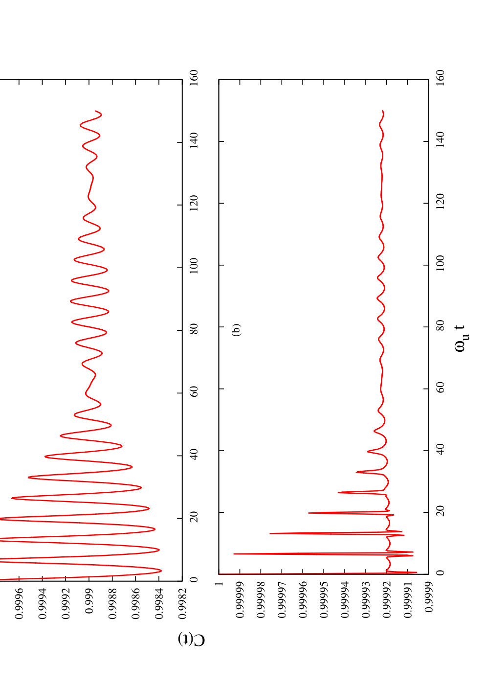
Refer to caption

Figure 7: Time variation of coherence factor C(t) at J⟂ωu=.05\frac{J_{\perp}}{\omega_{u}}=.05 and ωlωu=.9\frac{\omega_{l}}{\omega_{u}}=.9 for (a) g=1g=1 and (b) g=4g=4.

Here, we have considered a continuous uniform distribution of ωk\omega_{k} within a small region characterized by ωl≤ωk≤ωu\omega_{l}\leq\omega_{k}\leq\omega_{u}. As a consequence of the non-vanishing width ωu−ωl\omega_{u}-\omega_{l}, the harmonics in equations (115)–(117) do not all rephase at the same time (for t>0t>0) since they will always interfere destructively producing no scope for complete recoherence (recoherence is only obtained when one deals with a single phonon frequency). We will now explain the figures (7) and (8). Since the upper and the lower cutoff frequencies (i.e., ωu\omega_{u} and ωl\omega_{l}) are quite close to each other, beating effects are seen in the figures; the factor sin⁡[(ωu−ωl)​t′′2]\sin\Big[\frac{(\omega_{u}-\omega_{l})t^{\prime\prime}}{2}\Big] [with the beat frequency (ωu−ωl)(\omega_{u}-\omega_{l})] produces an envelope for the larger frequency oscillation produced by cos⁡[(ωu+ωl)​t′′2]\cos\Big[\frac{(\omega_{u}+\omega_{l})t^{\prime\prime}}{2}\Big] and sin⁡[(ωu+ωl)​t′′2]\sin\Big[\frac{(\omega_{u}+\omega_{l})t^{\prime\prime}}{2}\Big] [see equations () and ()]. The period of the envelope and the faster oscillation are given by Tenvl=2​πωu−ωlωu=20​πT_{\rm envl}=\frac{2\pi}{\frac{\omega_{u}-\omega_{l}}{\omega_{u}}}=20\pi and Tfast=2​πωu+ωl2​ωu=4019​πT_{\rm fast}=\frac{2\pi}{\frac{\omega_{u}+\omega_{l}}{2\omega_{u}}}=\frac{40}{19}\pi, respectively; thus, one period TenvlT_{\rm envl} of the envelope contains 192\frac{19}{2} (i.e., ωu+ωl2ωu−ωl=192\frac{\frac{\omega_{u}+\omega_{l}}{{2}}}{\omega_{u}-\omega_{l}}=\frac{19}{2} ) faster oscillations. At small values of ωu​t′′\omega_{u}t^{\prime\prime}, the nature of the plot is similar to the case when only one single phonon mode ω\omega is considered. The beating effect is not observed at smaller time as limωu​t′′→0sin⁡(ωu−ωl)​t′′2(ωu−ωl)​t′′2=1\lim_{\omega_{u}t^{\prime\prime}\rightarrow 0}\frac{\sin\frac{(\omega_{u}-\omega_{l})t^{\prime\prime}}{2}}{\frac{(\omega_{u}-\omega_{l})t^{\prime\prime}}{2}}=1 and we get oscillations with frequency ωu+ωl2≈ωu\frac{\omega_{u}+\omega_{l}}{2}\approx\omega_{u}. As ωu​t′′\omega_{u}t^{\prime\prime} increases from zero value, the factor sin⁡(ωu−ωl)​t′′2(ωu−ωl)​t′′2\frac{\sin\frac{(\omega_{u}-\omega_{l})t^{\prime\prime}}{2}}{\frac{(\omega_{u}-\omega_{l})t^{\prime\prime}}{2}} decreases and contributes very little at values of ωu​t′′\omega_{u}t^{\prime\prime} beyond 40​π40\pi. Consequently, the amplitude of the oscillations, in the exponent of the equations () and (121), decreases rapidly as ωu​t′′\omega_{u}t^{\prime\prime} increases from zero value. In the oscillations of figures (7) and (8), this describes the damping due to the non-vanishing width of the frequency distribution.

Refer to caption

Figure 8: Time variation of inelastic factor P(t) at J⟂ωu=.05\frac{J_{\perp}}{\omega_{u}}=.05 and ωlωu=.9\frac{\omega_{l}}{\omega_{u}}=.9 for (a) g=1g=1 and (b) g=4g=4.

References

  • [1] P. Zanardi and M. Rasetti, Phys. Rev. Lett. 79, 3306 (1997).
  • [2] J. Kempe, D. Bacon, D. A. Lidar, and K. B. Whaley, Phys. Rev. A 63, 042307 (2001).
  • [3] D. A. Lidar and K. B. Whaley, e-print arXiv quant-ph:0301032v1.
  • [4] B. Misra and E. C. G. Sudarshan, J. Math. Phys. 18, 756 (1977).
  • [5] A. G. Kofman and G. Kurizki, Nature 405, 546 (2000).
  • [6] P. Fachhi and S. Pascazio, J. Phys. A: Math. Theor. 41, 493001 (2008).
  • [7] D. Rossini, P. Facchi, R. Fazio, G. Florio, D. A. Lidar, S. Pascazio, F. Plastina, and P. Zanardi, Phys. Rev. A 77, 052112 (2008).
  • [8] L. Viola, Journal of Modern Optics 51, 2357 (2004).
  • [9] J. J. L.Morton, A. M. Tyrishkin, A. Ardavan, S. C. Benjamin, k. Porfyrakis, S. A. Lyon, and G. A. D. Briggs, Nature Physics 2, 40 (2006).
  • [10] L. Viola and S. Lloyd, Phys. Rev. A 58, 2733 (1998).
  • [11] U. Hohenester, J. Phys. B: At. Mol. Opt. Phys. 40, 315 (2007).
  • [12] J. J. L. Morton, D. R. McCamey, M. A. Eriksson, and S. A. Lyon, Nature 479, 345 (2011).
  • [13] J. R. Petta, A. C. Johnson, J. M. Taylor, E. A. Laird, A. Yacoby, M. D. Lukin, C. M. Marcus, M. P. Hanson, and A. C. Gossard, Science 309, 2180 (2005).
  • [14] H. Bluhm, S. Foletti, I. Neder, M. Rudner, D. Mahalu, V. Umansky, and A. Yacoby, Nature Physics 7, 109 (2011).
  • [15] B. M. Maune, M. G. Borselli, B. Huang, T. D. Ladd, P. W. Deelman, K. S. Holabird, A. A. Kiselev, I. Alvarado-Rodriguez, R. S. Ross, A. E. Schmitz, M. Sokolich, C. A. Watson, M. F. Gyure, and A. T. Hunter, Nature 481, 344 (2012).
  • [16] C. Barthel, J. Medford, C. M. Marcus, M. P. Hanson, and A. C. Gossard, Phys. Rev. Lett. 105, 266808 (2010).
  • [17] J. Levy, Phys. Rev. Lett. 89, 147902 (2002).
  • [18] I. G. Lang and Y. A. Firsov, Zh. Eksp. Teor. Fiz. 43, 1843 (1962) [Sov. Phys. JETP 16, 1301 (1962)].
  • [19] L.-A. Wu and D. A. Lidar, Phys. Rev. Lett. 91, 097904 (2003).
  • [20] A. Lanzara, N. L. Saini, M. Brunelli, F. Natali, A. Bianconi, P. G. Radaelli, and S. -W. Cheong, Phys. Rev. Lett. 81, 878 (1998).
  • [21] D. Louca, T. Egami, E. L. Brosha, H. Röder, and A. R. Bishop, Phys. Rev. B 56, R8475 (1997).
  • [22] A. J. Millis, P. B. Littlewood, and B. I. Shraiman, Phys. Rev. Lett. 74, 5144 (1995).
  • [23] S. Datta, A. Das, and S. Yarlagadda, Phys. Rev. B 71, 235118 (2005).
  • [24] J. R. Schrieffer and P. A. Wolff, Phys. Rev. 149, 491 (1966).
  • [25] S. Reja, S. Yarlagadda, and P. B. Littlewood, Phys. Rev. B 84, 085127 (2011).
  • [26] H.-P. Breuer and F. Petruccione, The Theory of Open Quantum Systems (Oxford University Press, Oxford, New York, 2007).
  • [27] F. Casas, A. Murua,and M. Nadinic, Computer Physics Communications 183, 2386 (2012).
  • [28] T. Yu and J.H. Eberly, Phys. Rev. B 66, 193306 (2002).
  • [29] R. Pankaj and S. Yarlagadda, Phys. Rev. B 86, 035453 (2012).
  • [30] K. D. Petersson, C. G. Smith, D. Anderson, P. Atkinson, G. A. C. Jones, and D. A. Ritchie, Nano Lett. 10, 2789 (2010).
  • [31] K. D. Petersson, J. R. Petta, H. Lu, and A. C. Gossard, Phys. Rev. Lett. 105, 246804 (2010).
  • [32] Qing-Shou Tan, Yong Dong, and Le-Man Kuang, Commun. Theor. Phys. (Beijing, China) 53, 71 (2010).
  • [33] L. Vidmar, J. Bonča, M. Mierzejewski, P. Prelovšek, and S. A. Trugman, Phys. Rev. B 83, 134301 (2011).
  • [34] E. Dagotto, T. Hotta, and A. Moreo, Phys. Rep. 344, 1 (2001).
  • [35] Y.-F. Yang and K. Held, Phys. Rev. B 76, 212401 (2007).