The Effect of Diffusion on the Particle Spectra in Pulsar Wind Nebulae

The general transport equation for a massive particle species, expressed as a function of momentum $p$ and the omnidirectional distribution function $f(\mathbf{r},p,t)$, is given by [12, 27, e.g.]

where

is the differential current density describing convection and diffusion, with $\mathbf{V}$ denoting the convection velocity and $\mathbf{\underline{K}}$ the diffusion tensor. The relationship between the omnidirectional distribution function and the more frequently used particle density is given by $N(\mathbf{r},p,t)=4\pi p^{2}f(\mathbf{r},p,t)$, where $N$ is defined as the number of particles per unit volume in the momentum interval $p+dp$. The expressions for synchrotron and inverse Compton emission spectra are usually stated in terms of $N(\mathbf{r},p,t)$ [2, 22, e.g.], whereas it is often more convenient to express transport equations in terms of $f(\mathbf{r},p,t)$.

The Compton-Getting coefficient [13, 14, e.g.]

takes into account that an observer moving relative to the rest frame in which $f$ is homogeneous and isotropic will measure a modified current density. This modification produces a spectral effect similar in nature to the Doppler effect on photons. For a power-law spectrum $f\propto p^{-(\alpha+2)}$, the coefficient has the value $C=(\alpha+2)/3$.

In a spherically expanding medium, energy or momentum losses include the adiabatic loss rate

However, [15] showed that when the particles reside in a wind with velocity $\mathbf{V}$, this is the momentum loss rate in the frame moving with the wind, while the loss rate in the stationary frame of reference is

The modification of the convective streaming from $\mathbf{V}f$ to $C\mathbf{V}f$, and the adiabatic cooling rate from (4) to (5), produces effects in the transport equation that cancel each other. [15] showed that when $C$ is dropped in $\mathbf{S}$, the momentum loss rate in (1) transforms from (5) back to its more familiar form. It should be noted at this point that the process of first-order Fermi acceleration in shocks is formally included in the transport equation if it is treated as a discontinuous jump in the flow velocity.

Synchrotron radiation and inverse Compton scattering in the Thomson regime have the same momentum dependence, making it possible to describe both non-thermal processes by the single expression

where

is a function of the magnetic ($U_{B}$) and photon ($U_{\rm{IC}}$) energy field densities. The other constants in (7) are $\sigma_{\rm{T}}$, the Thomson scattering cross-section, $m_{0}$, the rest mass of the particle, and $c$, the speed of light. In systems where $U_{\rm{IC}}>U_{B}$, (6) must be modified to take into account Klein-Nishina effects. Neglecting convection and diffusion, [24] solved (1) time-independently, finding that Klein-Nishina effects are still negligible if $U_{\rm{IC}}/U_{B}\lesssim 3$. For the CMBR with an energy density of $0.3$ $\rm{eV}/\rm{cm}^{3}$, this condition is satisfied for an average magnetic field of $\bar{B}>2$ $\mu\rm{G}$.

The term $D_{p}\partial f/\partial p$ describes stochastic or second-order Fermi acceleration in magnetohydrodynamic turbulence, with $D_{p}$ acting as the momentum diffusion coefficient. Lastly, any sources or sinks are included in the transport equation through $Q(\mathbf{r},p,t)$.

Inserting the above expressions for $\mathbf{S}$ and $\langle\dot{p}\rangle_{\rm{total}}=\langle\dot{p}\rangle_{\rm{ad}}+\langle\dot{p}\rangle_{\rm{n-t}}$ into (1), imposing spherical symmetry ($\partial f/\partial\phi=\partial f/\partial\theta=0$) on the system, and neglecting momentum diffusion, $D_{p}\partial f/\partial p=0$, leads to

expressed in the spherical coordinate $r$. In this case $\mathbf{\underline{K}}$ reduces to a single effective isotropic diffusion coefficient $\kappa(p,r,t)$.

To keep the model as general as possible, it is useful to scale the variables present in (8) to dimensionless ones. For radial distance, the scaling

is used, where $\tilde{r}$ is the unscaled variable and $\tilde{r}_{S}$ a characteristic length, chosen as the size of the system. This leads to a system with a scaled radial dimension of $0<r\leq 1$. A similar scaling is used for momentum

with the difference that $\tilde{p}_{S}$ is not chosen as the maximum particle momentum, but rather an intermediate value. For the present paper, the scaled momentum range is chosen as $10^{-3}\leq p\leq 10^{4}$. It is also possible to scale the particle energy in a similar fashion, $E=\tilde{E}/\tilde{E}_{S}$. Since $\tilde{E}=\tilde{p}c$ for relativistic particles, it follows that $E=p$. For the numerical calculations the scale energy is chosen as $\tilde{E}_{S}=1$ TeV, with the scaled momentum range translating to the energy range $1\mbox{ GeV}\leq\tilde{E}\leq 10$ PeV. This energy range includes the electron energy range needed to produce the non-thermal emission observed from PWN’e.

The convection velocity in the system is expressed as a fraction of the speed of light

while the diffusion diffusion coefficient is scaled as

It is useful to define a scaling factor for time, chosen as the light transition time through the system

Consequently, the non-thermal energy loss coefficient (7) is scaled as

The amount of energy lost by a particle is directly related to the residence time in the system. In the absence of diffusion, the convection time-scale is given by

Conversely, the diffusion time-scale, as derived by [27], is

It should be noted that diffusion is a stochastic process, and that $\tau_{\rm{dif}}$ represents an average propagation time. Furthermore, this diffusion time-scale is derived under the assumption that $\kappa$ is independent of $r$, and that the particles undergo negligible energy losses during propagation. The synchrotron cooling time is estimated to be [4, e.g.]

Magnetohydrodynamic (MHD) simulations show a complicated flow and magnetic field structure in PWN’e [20, 5, e.g.]. However, in the present one-dimensional problem a radial flow and azimuthal magnetic field is assumed, similar to the models of (e.g.) [31] and [18]. The latter assumption follows from the result that a radial plasma wind originating from a magnetised, rotating object leads to an Archimedean spiral structure in the magnetic field [27, e.g.]. As a result of the large rotational velocity of pulsars, the spiral structure can be approximated to a high degree as purely azimuthal [e.g. 19, and references therein].

It is further assumed that the ideal MHD limit

holds, allowing one to relate the radial profiles of the velocity and magnetic field. With the chosen flow and magnetic field structure, (18) reduces to

The convective flow downstream of the pulsar wind termination shock is subsonic, with the sound speed in a magnetised plasma being of the order $c/\sqrt{3}$ [32, e.g.]. The inner boundary of the computational domain is placed at the termination shock, where the velocity is chosen as $\tilde{V}_{0}=0.3c$. Steady-state MHD simulations [18] find that the radial velocity profile depends on the ratio of electromagnetic to particle energy, $\sigma$. When $\sigma=1$, the velocity remains almost independent of $r$. When $\sigma=0.01$, the velocity falls off as $V\propto 1/r^{2}$ close to the termination shock, but decelerates at one termination shock radius, and approaches a constant value at a radius that is a hundred times larger than the termination shock radius. For the current model a $V\propto 1/r^{0.5}$ profile is chosen. The same profile has been derived by [39] for HESS J1825-137.

The chosen velocity profile, together with (19), implies the magnetic profile $B\propto 1/r^{0.5}$, similar to the scaling $B\propto 1/r^{0.7}$ derived by [39]. Although the radial dependencies of $V$ and $B$ may be more complicated, the chosen profiles lead to a decrease in the velocity and magnetic field qualitatively similar to the large-scale structure calculated by [18].

For the magnetic field it is difficult to specify a characteristic value for PWN’e. The Crab Nebula has an average magnetic field strength of $\bar{B}\sim 300$ $\mu$G [38, e.g.], whereas it is estimated that the Vela PWN has a lower value of $\bar{B}\sim 3$ $\mu$G [4, e.g.]. For the numerical simulations, the value $\tilde{B}_{0}=350$ $\mu$G is chosen as the magnetic field strength at the inner boundary. This is again similar to the value $\tilde{B}_{0}\approx 400$ $\mu$G derived for HESS J1825-137 [39].

It is generally assumed [21, e.g.] that the radial ($\kappa_{r}$) and momentum ($\kappa_{p}$) dependence of the diffusion coefficient can be separated, $\kappa(r,p)=\kappa_{0}\kappa_{r}\kappa_{p}$, with $\kappa_{0}$ a constant. Diffusion occurs as a result of particle interaction with irregularities in the magnetic field, and experience with the propagation of cosmic rays in the heliosphere shows that the radial dependence of the diffusion coefficient can be modelled as $\kappa_{r}\propto 1/B$ [e.g. 3, and references therein]. This leads to the radial dependence $\kappa_{r}\propto r^{0.5}$ in the model. It has further been found that the momentum dependence of particles in the heliosphere scales as $\kappa_{p}\propto p$ [e.g. 3, and references therein]. The momentum dependence $\kappa_{p}=\tilde{p}/\tilde{p}_{S}$ is thus chosen in the model.

To account for the loss of particles with $\tilde{E}>100$ GeV from the gamma-ray emission region in the Vela PWN, a spatially-independent diffusion coefficient $\tilde{\kappa}_{0}\sim 10^{26}$ $\rm{cm}^{2}/s$ has been estimated by [16]. A similar $\tilde{\kappa}_{0}$ has also been derived by [39] to explain TeV gamma-ray emission from the source HESS J1825-137. For a PWN size $\tilde{r}_{S}=10$ pc and $\tilde{E}_{S}=\tilde{p}_{S}c=1$ TeV, the coefficient $\kappa$ has the same value as the observationally derived value when $\kappa_{0}=10^{-3}$ and $\tilde{E}=100$ GeV. For the purpose of illustration, the smaller value $\kappa_{0}=4\times 10^{-5}$ is chosen at the inner boundary, and is motivated by the scaling $\kappa\propto 1/B$. Since the average magnetic field in the model is larger than $\bar{B}$ in the Vela PWN, a smaller diffusion coefficient is appropriate. With the radial scaling taken into account (fixed by the radial profile of the magnetic field), the diffusion coefficient varies from $\kappa=4\times 10^{-5}E$ at the inner boundary, to $\kappa=4\times 10^{-4}E$ at the outer boundary.

Lastly, the particle energy spectrum injected by the source is chosen as $f(p,r_{0})\propto p^{-4}$, or in terms of the differential particle density $N\propto p^{-2}$. This is the index of the particle spectrum needed to explain the X-ray emission observed in the vicinity of the termination shock [e.g. 10, and references therein]. Since the particles are relativistic ($\tilde{E}=\tilde{p}c$), and with the scaling of the parameters described in Section II.2, the source spectrum can also be expressed as $N\propto\tilde{E}^{-2}$.

This section presents two sets of steady-state solutions to (8). The first set includes only the processes of convection and adiabatic losses, while the second set includes convection, together with adiabatic and synchrotron losses. For convenience, the former scenario will be referred to as the convection scenario, while the latter will be referred to as the convection-synchrotron scenario. Figure 1 shows the spectra for the convection scenario, together with the convection-synchrotron scenario. When diffusion and synchrotron losses are absent, the spectra shift to lower energies as a result of adiabatic losses, while retaining the spectral shape of the source spectrum. This can be demonstrated analytically as follows: for the steady-state convection scenario with a radially independent $V=V_{0}$, the transport equation (8) simplifies to

Using the method of characteristics to solve the above equation, one finds that the solutions to (23) are constant along the contours

in the $(r,p)$-plane, valid for any choice of source function. With the boundary condition (22) taken into account, this leads to the solution

where $\mathcal{H}$ is the Heaviside function.

The analytical solution (25) shows that the spectra at any position in the system have the same $p$-dependence as the source spectrum, with the only difference being that the intensities are reduced. This behaviour can be ascribed to the fact that the fractional momentum change as a result of adiabatic losses, (5), is independent of momentum. The same result has also been found by (e.g.) [17] and [21].

The analytical result (25) is a useful baseline for obtaining an estimate of the accuracy of the numerical scheme. Using a radially-independent velocity, it was found that the numerical solutions are within $10\%$ of the analytical solutions in the inner part of the system. The accuracy decreases as a function of position, so that at $r=0.9$ the intensity of the numerical spectrum is a factor two below the analytical result. When diffusion is absent, the character of (8) changes from parabolic to hyperbolic, and the Crank-Nicolson method is no longer the most suitable scheme for solving (8). However, at $r=0.9$ the intensity has dropped a factor of $10^{5}$ compared to the source spectrum, (see Figure 1), and a factor of two becomes negligible.

Including the effect of synchrotron losses leads to the familiar cut-off that shifts to lower energies with increasing $r$, as shown in Figure 1. Additionally, a small peak is visible just before the cut-off in the spectrum at $r=0.9$. The most intuitive explanation for this peak would be that synchrotron losses lead to a pile-up of particles at the edge of the cut-off. Such an effect is indeed expected for the source spectrum $N\propto p^{-\alpha}$ when $\alpha<2$ [22, e.g.]. However, the peak in Figure 1 (where the source spectrum has $\alpha=2$) is not a physical effect, but rather a numerical artefact resulting from the absence of diffusion. The difference between the intensities of the peak and the adiabatic part of the spectrum ($\tilde{E}\lesssim 1.4$ TeV) is the factor two mentioned in the previous paragraph. When diffusion is included in the problem, (cf. Figure 2), the correct intensity is calculated.

The energy, $\tilde{E}_{\rm{syn}}$, where the synchrotron break should appear can be estimated by equating the right-hand sides of (15) and (17), and then solving for $\tilde{E}$. The value for the magnetic field used in the estimate is the average value in the region ranging from $r_{0}$ to $r$. This leads to the estimates $\tilde{E}_{\rm{syn}}\sim 12.6$ TeV at $r=0.1$ and $\tilde{E}_{\rm{syn}}\sim 2.9$ TeV at $r=0.9$. The break energies in Figure 1 are located at the lower energies $\tilde{E}\sim 6$ TeV and $\tilde{E}\sim 1.4$ TeV for $r=0.01$ and $r=0.9$, respectively. A comparison of the numerical results with the order-of-magnitude estimates shows a factor $2$ difference in the break energies, confirming the validity of the numerical scheme.

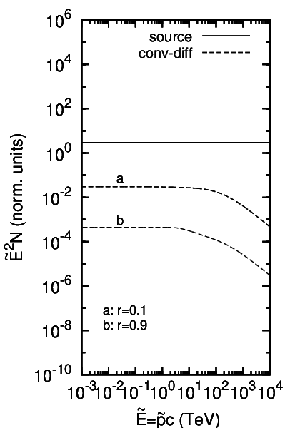
To determine the effect of diffusion on the evolution of the particle spectrum, this section considers steady-state solutions to (8), i.e. $\partial f/\partial t=0$, with the processes of convection, diffusion and adiabatic losses included. The values for the parameters are as discussed in Section II.4. The evolution of the spectra in a convection-diffusion system can be divided into two regimes, as shown in Figure 2. At lower energies convection and adiabatic losses dominate and the spectra retain the shape of the source spectrum. At higher energies diffusion is more important, leading to an evolution in the spectral index. With the free-escape (Dirichlet) condition imposed at the outer boundary, the diffusion-dominated part of the spectra become softer by one power-law index, $N\propto p^{-3}$, or expressed in terms of energy, $N\propto\tilde{E}^{-3}$ (see Section II.2).

This softening of the spectra is typical of escape losses [1, e.g.], and is related to the momentum dependence of the diffusion coefficient. For the general case $\kappa\propto p^{\lambda}$, the diffusion-dominated part of the spectra is described by $N\propto p^{-\alpha-\lambda}$ [17, 21, 1, e.g.], with $\alpha=2$ and $\lambda=1$ in the present model.

In the outer part of the system, $r=0.9$, the transition between the two regimes is more gradual, compared to the transition at $r=0.1$. Particles with $\tilde{E}\lesssim 20$ TeV are transported predominantly by convection in the inner part of the system. However, since the diffusion coefficient increases with radial distance, the energy where particles are transported by convection has reduced to $\tilde{E}\lesssim 4$ TeV at $r=0.9$. Particles in the energy range $4\mbox{ TeV}\lesssim\tilde{E}\lesssim 20$ TeV have been subjected to reduced adiabatic losses, compared to the particles at $\tilde{E}\lesssim 4$ TeV, leading to the more gradual transition at $r=0.9$.

The importance of diffusion relative to convection can be estimated using the Péclet number [30, e.g.]

When $\xi\gg 1$ the system is convection dominated, while being diffusion dominated for $\xi\ll 1$. Note that $\xi$ is in essence the ratio of the convection and diffusion time-scales, (15) and (16). With the ideal MHD limit imposed and assuming that $\kappa_{r}\propto 1/B$ (see Section II.4), the scaling $V=V_{0}(r_{0}/r)^{\beta}$ implies the scaling $\kappa=\kappa_{0}(r/r_{0})^{(1-\beta)}\kappa_{p}$. Inserting these radial profiles into (26) leads to

where it will be recalled from Section II.4 that $\kappa_{p}=\tilde{p}/\tilde{p}_{S}$. It thus follows from (27) that the value of $\xi$ is not uniquely defined for the system. For the low energy part of the spectrum in Figure 2, one has $\xi>1$, while $\xi<1$ at high energies. The energy, $\tilde{E}_{\rm{dif}}=\tilde{p}_{\rm{dif}}c$, where the two transported process are equal can be found by setting $\xi=1$. Using the values of $V_{0}$ and $\kappa_{0}$ chosen for the numerical calculations lead to the estimate $\tilde{E}_{\rm{dif}}\sim 75$ TeV. This is in fair agreement with the values of $\tilde{E}_{\rm{dif}}\sim 100$ TeV at $r=0.1$ and $\tilde{E}_{\rm{dif}}\sim 40$ TeV at $r=0.9$, which once again confirms the validity of the numerical scheme.

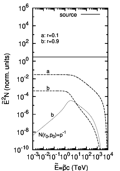
The last step is to determine the effect of diffusion on the evolution of the spectra when synchrotron losses are present. This section considers steady-state solutions to (8), with the transport processes of convection and diffusion included, together with adiabatic and synchrotron energy losses. The results are plotted in Figure 3.

Compared to the convection system in Figure 1, diffusion decreases the propagation time of particles through the system, thereby reducing the amount of synchrotron losses suffered by the particles. The particles that lose the most energy due to synchrotron radiation are generally the particles with the largest diffusion coefficient, leading to a significant moderation of the characteristic synchrotron cut-off, as shown in Figure 3.

The spectrum at $r=0.1$ transitions from the adiabatic-dominated part at an energy $\tilde{E}\sim 5$ TeV, almost identical to the cut-off energy $\tilde{E}_{\rm{syn}}\sim 6$ TeV in Figure 1. The spectrum then softens to $N\propto\tilde{E}^{-3}$ at a slightly larger energy $\tilde{E}\sim 20$ TeV. This is also the energy where the effect of diffusion becomes visible in Figure 2. A comparison of the diffusion-dominated part of the spectra shows that the intensity in Figure 3 is lower than the corresponding intensity in Figure 2. The particles at $r=0.1$ in Figure 3 have undergone a significant amount of synchrotron losses, but the shape of the spectrum is nevertheless determined by diffusion. The exception is at very high energies, where a synchrotron cut-off appears.

At $r=0.9$ a more pronounced effect between the importance of diffusion, relative to synchrotron losses, can be seen. The transition from the adiabatic-dominated part again occurs at an energy $\tilde{E}\sim 1$ TeV that is similar to $\tilde{E}_{\rm{syn}}\sim 1.4$ TeV in Figure 1. In the energy range $1\mbox{ TeV}\lesssim\tilde{E}\lesssim 10$ TeV the spectrum initially softens, and can be fitted with a power-law $N\propto\tilde{E}^{-3.8}$. This initial softening of the spectrum is followed by a marginal harder spectrum at $\tilde{E}\sim 10$ TeV. This is also the energy where the effect of diffusion becomes visible in Figure 2. In the energy range $10\mbox{ TeV}\lesssim\tilde{E}\lesssim 200$ TeV the spectrum can be fitted with the power law $N\propto\tilde{E}^{-3.5}$. At $\tilde{E}\gtrsim 100$ TeV the spectrum softens again, signifying the beginning of the high-energy cut-off. Although one might be inclined to believe that the effect of diffusion on synchrotron losses would only be important for $\tilde{E}\gtrsim 10$ TeV, Figure 3 shows that diffusion already reduces the amount of synchrotron losses for $\tilde{E}\lesssim 10$ TeV.

Shown for comparison is the spectrum at $r=0.9$ for a $N\propto p^{-1}$ source spectrum. For the purpose of clarity, this spectrum has been divided by a factor $10^{3}$. The spectrum can be fitted with a power-law $N\propto\tilde{E}^{-3}$ in the energy range $10\mbox{ TeV}\lesssim\tilde{E}\lesssim 200$ TeV.

While the spectra shown if Figures 1-3 were calculated using a free-escape outer boundary condition, it may be argued that a realistic scenario should have a partial escape boundary. To investigate the influence of the outer boundary on the spectra, a no-escape condition ($\mathbf{S}=0$) was also imposed on the convection-diffusion-synchrotron scenario, where it was found that the choice of outer boundary condition does not affect the solutions. When energy losses are present, particles not only escape in radial, but also momentum space, and the choice of outer boundary condition becomes unimportant. This is especially true for the high-energy particles for which synchrotron losses are important.

Observations of the Vela PWN, located at a distance of $290$ pc [7], show a bright X-ray nebula surrounding the termination shock [23]. The synchrotron photon index, $\Gamma$, in the $3-10$ keV range was extracted from a number of annular regions of increasing size, revealing a softening of the index with increasing distance from the shock, located at $r_{\rm{ts}}=0.35^{\prime}$ [26]. In the inner region, $r\leq 0.5^{\prime}$, the photon index was found to be $\Gamma=1.5\pm 0.02$, while in the outer annular region $8^{\prime}\leq r\leq 12^{\prime}$, the index was found to be $\Gamma=1.9\pm 0.06$. If the energy spectrum of the particles is described by $N\propto E^{-\alpha}$, then the relation $\Gamma=(\alpha+1)/2$ implies $\alpha=2\pm 0.04$ in the inner region, and $\alpha=2.8\pm 0.12$ in the outer annular region. A similar X-ray observation ($0.5-9$ keV) has also been performed for the nebula MHS 15-52, located at a distance of $5.2\pm 1.4$ kpc [9]. In the inner annular region, $30^{\prime\prime}\leq r\leq 57^{\prime\prime}$, the photon index was was found to be $\Gamma=1.66\pm 0.02\hskip 5.69046pt(\alpha=2.32\pm 0.04)$, softening to $\Gamma=2.24\pm 0.28\hskip 5.69046pt(\alpha=3.48\pm 0.56)$ in the outer annular region, $246^{\prime\prime}\leq r\leq 300^{\prime\prime}$ [33].

The electron energy, $\tilde{E}$, needed to produce a synchrotron photon with a keV energy, $\tilde{E}_{\rm{keV}}$, is [4]

With the parameters chosen in Section II.4, the magnetic field has the values $\tilde{B}_{r=0.1}=113$ $\mu$G, and $\tilde{B}_{r=0.9}=38$ $\mu$G. Inserting these values into (28), one finds that the electron energy needed to produce synchrotron emission in the range $\tilde{E}_{\rm{keV}}=0.5-10$ keV is $\tilde{E}_{r=0.1}=15-65$ TeV and $\tilde{E}_{r=0.9}=25-113$ TeV. Figure 3 shows that these are the particle energy ranges where diffusion will have the largest influence on the evolution of the spectra. Furthermore, the index $\alpha_{r=0.9}=3.5$ derived from Figure 3 (in the energy range $2\mbox{ TeV}\lesssim\tilde{E}\lesssim 100$ TeV) is consistent with the observed index in the outer regions of MSH 15-52. Selecting a wind profile $V\propto 1/r^{0.1}$, while keeping all the other parameters fixed (see Section II.4), the model calculates a particle index $\alpha_{r=0.9}=2.8$, in agreement with the observed index in the outer regions of the compact Vela PWN.

It should be kept in mind that the observations represent an average of the particle spectra in an annular region, whereas the results in Figure 3 show spectra at a given point. Even with this caveat in mind, the results from Figure 3 indicate that diffusion should play an important role in determining the photon index, and can help to explain the observed softening of the spectrum.

To demonstrate the solutions obtained with the numerical scheme, the initial condition is chosen as an empty system. For this simulation, only convection, diffusion, and adiabatic losses are taken into account. Additionally, any time-dependence in the coefficients is neglected, while the outer boundary remains static. The source is switched on at $t=0$, and the system is allowed to reach a steady-state.

Figure 4 shows the evolution of the spectra at three different times, with the system having reached a steady-state at $t=50$. At times $t=15$ and $t=30$, the spectra at $r=0.1$ already resemble the steady-state spectrum (cf. Figure 2). This is also true for the high-energy part of the spectra at $r=0.9$. However, at lower energies the spectra develop a cut-off that decreases in energy with increasing time. Particles with energies below this cut-off cannot propagate as effectively to the outer parts of the system as a result of a small diffusion coefficient. The energy where the cut-off should appear can be estimated using the diffusion time-scale, (16). Using the average value of $\kappa$ between $r_{0}$ and $r=0.9$ leads to the estimate $\tilde{E}\sim 40$ TeV for $t=15$, and $\tilde{E}\sim 20$ TeV for $t=30$, in good agreement with the values shown in Figure 4. This demonstrates the soundness of the numerical scheme.

In this section the effect of time-dependent coefficients on the evolution of the spectra is illustrated. The processes of convection, diffusion, as well as both energy loss mechanisms, i.e. adiabatic expansion and synchrotron radiation, are included. An initially empty system is allowed to reach a steady-state at $t_{0}=50$ (cf. Figure 3), before the time-dependence $B_{0}\propto 1/t$ and $\kappa_{0}\propto t$ is introduced.

Figure 5 shows the spectra as a function of time, for $t=100$ $(2\times t_{0})$ and $t=150$ $(3\times t_{0})$. At $r=0.9$ the time-dependence is much more pronounced than at $r=0.1$. With $B\propto 1/t$, the synchrotron loss rate, (7), decreases as $z\propto 1/t^{2}$, while the escape time, (16), decreases as $\tau_{\rm{dif}}\propto 1/t$. Since the amount of synchrotron losses is dependent on both $z$ and $\tau_{\rm{dif}}$, the change in the amount of synchrotron losses suffered is $\propto 1/t^{3}$. From $t_{0}=50$ to $t=100$ there is a rapid increase in the intensity, but from $t=100$ to $t=150$ the synchrotron losses have become so small that the intensity saturates.

The last scenario demonstrates the effect of a moving boundary. Figure 6 shows the solutions of (33) with the processes of convection, diffusion, adiabatic expansion, and synchrotron losses included. The velocity at the inner boundary is $\tilde{V}_{0}=0.3c$, while a constant expansion velocity, $\tilde{V}_{\rm{pwn}}=2000$ km/s, is chosen. The inner and outer boundaries are at $r_{0}=0.01$ and $r=1$, respectively, with the initial size of the system chosen as $\tilde{r}_{S}=1$ pc. The velocities at the boundaries imply a radial convection profile $V\propto 1/r^{0.83}$.

The value $\tilde{B}_{0}=500$ $\mu$G is chosen at the inner boundary of the system, with the radial scaling of the magnetic field determined using the ideal MHD limit, (19). The radial profile of the magnetic field is therefore given by $B\propto 1/r^{0.17}$. The diffusion coefficient has a value $\kappa_{0}=3\times 10^{-5}$, or in terms of the unscaled value, $\tilde{\kappa}_{0}=10^{24}$ $\rm{cm}^{2}/\rm{s}$. This is very similar to the value $\kappa_{0}=4\times 10^{-5}$ chosen for the steady-state simulations. The radial scaling of $\kappa_{r}$ is once again chosen as inversely proportional to the scaling of the magnetic field, implying $\kappa_{r}\propto r^{0.17}$.

To find an appropriate initial condition, the system is first allowed to reach a steady-state at $t_{0}=50$. Starting at $t=t_{0}$, the system then expands until $t=350$, representing a factor seven increase in the size of the system. Note that the spectra shown at the different times are plotted at the positions in the transformed, static system, i.e. at $r^{\prime}=0.1$ and $r^{\prime}=0.9$.

The first noticeable feature in Figure 6 is that the intensities in the convection-dominated part of the spectrum decrease with time. This is a direct result of the expansion of the system. Adiabatic losses scale as $V/r$ in a spherical system, leading to larger losses in the inner part of the system. This is also the reason why the amount of adiabatic losses at a given position in the static system, $r^{\prime}$, decreases with time. As $t$ increases, $r^{\prime}$ represents larger $r$ values in the PWN, leading to less adiabatic losses.

In the diffusion/synchrotron dominated regime, the spectra at $r^{\prime}=0.1$ become softer with increasing time, while the synchrotron cut-off at $\tilde{E}\sim 5000$ TeV shifts to lower energies. For increasing values of $t$ the particles have travelled further through the system, and have therefore been subjected to more synchrotron losses. In the first time interval, $50\leq t\leq 200$, the amount of losses is still significant. However, the decrease in $z$ is of such a nature that the amount of synchrotron losses is significantly reduced in the second time interval, $50\leq t\leq 200$.

At $r^{\prime}=0.9$ the spectra become marginally harder with time. Furthermore, the largest increase occurs in the second time interval. To understand this opposite behaviour, it is important to take into account all the contributing factors. Firstly, if the value of the diffusion coefficient remains unchanged, then a larger system leads to longer residence times, thereby reducing the relative importance of diffusion. However, this effect is partially offset by the fact that the system expands at a constant velocity. At times $t\geq t_{0}$ the velocity is described by the profile $V\propto 1/r^{\beta}$, with $\beta=0.83$. Since the velocity at the inner and outer boundaries remains constant, the index of the radial profile has evolved to $\beta=0.58$ at $t=350$. The scaling $B\propto 1/r^{1-\beta}$, together with the scaling $\kappa\propto 1/B$, implies that the diffusion coefficient becomes larger in the outer part of the system with increasing time, thereby counteracting the effect of longer residence times. Although the change in the index of the convective radial profile implies an identical change in the index of the magnetic field profile, the amount of synchrotron losses as a function of position decreases more rapidly. This is due to the $z\propto B^{2}$ dependence of the synchrotron loss coefficient, (7), leading to a change in the profile of $\Delta\beta=0.48$. The effect of synchrotron losses therefore decreases faster with time, becoming less important in the outer parts of the system.

In the absence of diffusion, one would expect expect the synchrotron cut-off to shift to lower energies with an increase in time. However, since the importance of diffusion increases with time, the effect is a marginal hardening of the spectrum. This hardening of the spectrum at $t=350$ is not caused by particles that were originally located at $r^{\prime}=0.9$ at $t_{0}=50$, but rather by particles that have diffused from distances $r^{\prime}<0.9$ to $r^{\prime}=0.9$ at times $t>50$.

The spectra at $t_{0}=50$ are the solutions that would have been found if (8) were solved time-independently, i.e. $\partial f/\partial t=0$. Thus, in summary, the moving boundary predominantly leads to a reduction in the intensity and radial particle gradients with time, but has a limited influence on the shape of the spectrum.

References

- [1] Atoyan, A. M., Aharonian, F. A., & Völk, H. J. 1995, Phys. Rev. D, 52, 3265
- [2] Blumenthal, G. R. & Gould, R. J. 1970, Rev. Mod. Phys., 42, 237
- [3] Caballero-Lopez, R. A., Moraal, H., McCracken, K. G., & McDonald, F. B. 2004, JGR, 109, 12102
- [4] De Jager, O. C. & Djannati-Ataï, A. 2009, in Astrophys. Space. Sci. Lib., Vol. 357, 451
- [5] Del Zanna, L., Amato, E., & Bucciantini, N. 2004, A&A, 421, 1063
- [6] Dobler, G. & Finkbeiner, D. P. 2008, ApJ, 680, 1222
- [7] Dodson, R., Legge, D., Reynolds, J. E., & McCulloch, P. M. 2003, ApJ, 596, 1137
- [8] Douglas, J. 1962, Numerische Mathematik, 4, 41
- [9] Gaensler, B. M., Brazier, K. T. S., Manchester, R. N., Johnston, S., & Green, A. J. 1999, MNRAS, 305, 724
- [10] Gaensler, B. M. & Slane, P. O. 2006, ARA&A, 44, 17
- [11] Gelfand, J. D., Slane, P. O., & Zhang, W. 2009, ApJ, 703, 2051
- [12] Ginzburg, V. L. & Syrovatskii, S. I. 1964, The Origin of Cosmic Rays (Pergamon Press)
- [13] Gleeson, L. J. & Axford, W. I. 1968, Ap&SS, 2, 431
- [14] Gleeson, L. J. & Urch, I. H. 1973, Ap&SS, 25, 387
- [15] Gleeson, L. J. & Webb, G. M. 1978, Ap&SS, 58, 21
- [16] Hinton, J. A., Funk, S., Parsons, R. D., & Ohm, S. 2011, ApJL, 743, L7
- [17] Jokipii, J. R. & Higdon, J. C. 1979, ApJ, 228, 293
- [18] Kennel, C. F. & Coroniti, F. V. 1984, ApJ, 283, 694
- [19] Kirk, J. G., Lyubarsky, Y., & Petri, J. 2009, in Astrophys. Space. Sci. Lib., Vol. 357, 421–450
- [20] Komissarov, S. S. & Lyubarsky, Y. E. 2003, MNRAS, 344, L93
- [21] Lerche, I. & Schlickeiser, R. 1981, ApJS, 47, 33
- [22] Longair, M. S. 1994, High Energy Astrophysics: volume 2 (Cambridge University Press)
- [23] Mangano, V., Massaro, E., Bocchino, F., Mineo, T., & Cusumano, G. 2005, A&A, 436, 917
- [24] Moderski, R., Sikora, M., Coppi, P. S., & Aharonian, F. 2005, MNRAS, 363, 954
- [25] Ng, C. K. & Gleeson, L. J. 1975, SoPh, 43, 475
- [26] Ng, C.-Y. & Romani, R. W. 2004, ApJ, 601, 479
- [27] Parker, E. N. 1965, Plan.&SS, 13, 9
- [28] Planck Collaboration. 2012, ArXiv:1208.5483
- [29] Potgieter, M. S. & Moraal, H. 1985, ApJ, 294, 425
- [30] Prandtl, L. 1953, Essentials of Fluid Dynamics (Blackie & Sons)
- [31] Rees, M. J. & Gunn, J. E. 1974, MNRAS, 167, 1
- [32] Reynolds, S. P. & Chevalier, R. A. 1984, ApJ, 278, 630
- [33] Schöck, F. M., Büsching, I., de Jager, O. C., Eger, P., & Vorster, M. J. 2010, A&A, 515, A109
- [34] Smith, E. J. 2001, JGR, 106, 15819
- [35] Steenberg, C. D. & Moraal, H. 1996, ApJ, 463, 776
- [36] Steenkamp, R. 1995, PhD thesis, Potchefstroom University for CHE
- [37] Su, M., Slatyer, T. R., & Finkbeiner, D. P. 2010, ApJ, 724, 1044
- [38] Trimble, V. 1982, Rev. Mod. Phys., 54, 1183
- [39] Van Etten, A. & Romani, R. W. 2011, ApJ, 742, 62
- [40] Venter, C., De Jager, O. C., & Clapson, A.-C. 2009, ApJ, 696, L52