Computational Aspects of Optional Pólya Tree
Abstract
Optional Pólya Tree (OPT) is a flexible non-parametric Bayesian model for density estimation. Despite its merits, the computation for OPT inference is challenging. In this paper we present time complexity analysis for OPT inference and propose two algorithmic improvements. The first improvement, named Limited-Lookahead Optional Pólya Tree (LL-OPT), aims at greatly accelerate the computation for OPT inference. The second improvement modifies the output of OPT or LL-OPT and produces a continuous piecewise linear density estimate. We demonstrate the performance of these two improvements using simulations.
Keywords: density estimation, Bayesian inference, recursive partition, smoothing, time complexity.
1 Introduction
Given independent random samples, characterizing a distribution is one of the most fundamental tasks in statistics. Density estimation is a key approach to solve such problems and is closely related to other problems such as clustering, classification and regression (Silverman, 1986; Scott, 1992; Hastie et al., 2009). Kernel density estimation (Rosenblatt, 1956; Parzen, 1962; Jones et al., 1996; Gray, 2003; Fan and Marron, 1994; Wand, 1994; Yang et al., 2003) and data-driven histograms (Scott, 1979; Barron et al., 1992; Lugosi and Nobel, 1996; Klemelä, 2009) are popular methods for non-parametric density estimation. Among many approaches developed for density estimation, non-parametric Bayesian models have the merits of being highly flexible and computationally feasible. Dirichlet process (Ferguson, 1973), Pólya tree (Ferguson, 1974) and their extentions are commonly used non-parametric Bayesian priors. Recently, Wong and Ma (2010) proposed an extension to the Pólya tree prior, named Optional Pólya Tree (OPT), which allows for optional stopping and random selection of partitioning variables. It has three attractive properties: 1) It fits the data adaptively; 2) It produces absolutely continuous distributions; and 3) The computation for exact OPT inference can be done in finite steps. OPT has been successfully applied in both one-sample (Wong and Ma, 2010) and two-sample (Ma and Wong, 2011) settings.
Albeit all these merits, there are existing issues which may hinder the application of OPT. Two major issues are: 1) The running time for exact OPT inference increases rapidly as sample size and the dimension of the data increase, which becomes prohibitive when the dimension is high; 2) OPT gives rise to piecewise constant densities11 1 The posterior mean of OPT gives a smooth density. However, its estimation is usually computationally prohibitive Wong and Ma (2010). The hierarchical maximum a posteriori (hMAP) estimate proposed by Wong and Ma (2010) is computationally more friendly, but gives rise to piecewise constant density estimates., where discontinuities occur at boundaries between the pieces, which could become undesirable for applications where smooth densities are sought.
In this paper we attempt to tackle the above two problems. In particular, we demonstrate that the computation for OPT inference can be greatly accelerated by performing approximate inference. We also present an approach which modifies the output of OPT and produces a continuous piecewise linear density estimate. This paper is organized as follows: In Section 2 we review the construction of OPT and the algorithm for its exact inference. In Section 3 we present an approach for reducing the computation named Limited-Lookahead Optional Pólya Tree (LL-OPT). Section 4 gives the time complexity analysis for OPT and LL-OPT. In Section 5 we present an approach for the estimation of smooth densities. Simulation studies are given in Section 6.
2 Optional Pólya Tree and its inference
Proposed by Wong and Ma (2010), OPT is an extension to the Pólya tree prior (Ferguson, 1974). OPT defines a procedure which gives rise to random probability measures on a space . In this paper we assume that is a bounded hyperrectangle in and is the Lebesgue measure. The theory of OPT applies to more general cases, e.g., is a counting measure when is finite.
The OPT procedure operates simultaneously as two processes: the first process recursively and randomly partitions the space and the second process recursively assigns a random probability measure into each region in the partition generated by the first process.
The recursive partitioning process works as follows: Starting from the root region , a random binary sample is drawn according to where is a parameter of the OPT. If , we stop further partitioning and mark it as a terminal region. If , a random integer is drawn according to a probability vector , where is the number of different ways of partitioning into subregions and is a set of parameters of the OPT such that . If , is partitioned in the -th way into subregions such that
The partitioning process is then recursively applied to each subregion of , and consequently, a partition tree is built by the process recursively. The partitioning process terminates when all the regions in the partition are marked as terminal regions.
The process for random assignment of probability measures works along with the partitioning process. It begins with a probability measure which is uniform within the root region . Whenever a region is partitioned into subregions , a random vector is drawn from a Dirichlet distribution with parameter and then a new probability measure is built based on by reassigning the probability mass within according to , were is the level of region in the partition tree with . Within each subregion , the probability mass is again uniformly distributed.
For the OPT procedure described above, there exists a limiting probability measure for (Wong and Ma, 2010, Theorem 1): If is uniformly bounded away from and for all , then converges almost surely in variational distance to a probability measure which is absolutely continuous with respect to . The density of with respect to on is piecewise constant with countably many pieces.
As a prior distribution on the space of probability measures, one merit of OPT is that the computation for exact OPT inference is analytically manageable. Given independent random samples from when has a OPT prior with independent stropping probabilities and all the parameters of are uniformly bounded away from and , the posterior distribution of is also an OPT with the following parameters (Wong and Ma, 2010, Theorem 3):
- 1.
Stopping probabilities:
- 2.
Selection probabilities:
- 3.
Probability mass allocation:
where are the numbers of samples in falling into each regions of the partition, , is the marginal likelihood of the data conditional on which can be calculated using the following recursive equation:
| (2.1) |
There are many different schemes for partitioning the regions. In this paper we consider a simple binary partitioning scheme proposed in Wong and Ma (2010): For , i.e., a hyperrectangle in , there are ways to partition . For the -th way, , we partition into two subregions at the midpoint of the range of such that and .
3 Acceleration of computation
According to (2.1), exact OPT inference requires computing recursively, which is computationally challenging since the running time increases rapidly as the dimension of the data increases. This is evident based on the fact that in (2.1) the value of has to be computed for every region with at least one data point and the number of such regions is enormous when the dimension is high. Figure 1 shows the running time for OPT inference for samples of various sizes and dimensions, using a fast algorithm for exact OPT inference which will be introduced Section 4. We can see that the running time increases nearly exponentially with respect to the dimension of the data and it becomes prohibitive when the dimension is or higher. The analysis of the time complexity for OPT inference is given in Section 4.
The computation for OPT inference can be greatly accelerated by performing the inference approximately. In a straightforward approach, named Naive Inexact Optional Pólya Tree (NI-OPT), we stop the recursion in (2.1) when the number of samples in a region is small or when the volume of is small, and compute by assuming that all the samples in are uniformly distributed and therefore no further partitioning of is necessary. The rationale for employing these heuristics is that when the volume of is small, error in is only likely to affect the estimated density locally, and when the number of samples in is small, would not be too different from which is computed by redistributing the samples in uniformly.
In practice, we found that the running time for the NI-OPT approach, although significantly reduced compared with the exact OPT approach, is still prohibitive when the sample size is large and when the dimension is high. In this paper we propose a more efficient algorithm for approximate OPT inference, named Limited-Lookahead Optional Pólya Tree (LL-OPT), which works as follows: starting from the root region , we perform the recursive computation in (2.1) for up to levels in the partition tree, where is a tuning parameter which provides a trade-off between running time and estimation accuracy. For a region at level , we stop the recursion and approximate as using the uniform approximation as we did in NI-OPT. Based on the computed and where are all the subregions of , we compute the hierarchical maximum a posteriori (hMAP) tree using the approach described in Wong and Ma (2010) for up to levels, where is another tuning parameter. In our implementation we fix . For each leaf node in the hMAP tree, we recursively apply the LL-OPT algorithm and build a sub-tree by treating that leaf node as the root node. Furthermore, like in NI-OPT, we can also stop the procedure when the number of samples in the region is small enough, or when the volume of the region is small enough.
4 Time complexity analysis for OPT and LL-OPT
In this section we study the time complexity for the exact OPT and the LL-OPT algorithms. For simplicity we consider only the simple binary partitioning scheme described in Section 2. However, the analysis technique may be adapted to more complicated partitioning schemes. For each region , the exact OPT algorithm according to (2.1) has to undertake the following three computational tasks:
For task 1, as , the straightforward way of counting the number of samples in each of the subregions of will take operations, where is the total number of samples in . However, this cost can be reduced by trading space for time. If we can store the set of samples in , counting the number of samples in each of the subregions of will only take operations, where is the number of samples in . Let denote the time for computing for a region with samples. The time complexity for task 2 is therefore . For task 3, the time complexity is if we assume that function can be computed in time. The time complexity for computing is therefore
| (4.1) |
It is shown in (4.1) that the value of depends on the values of and , which are determined by the distribution of samples within . The more uniformly the samples are distributed in , the less the computation time is required. Here we estimate for the following three cases:
- 1.
and , where is a constant.
- 2.
and , where is uniformly distributed within .
- 3.
and , where is a constant.
We see that case 2 represents a more realistic picture between the two extremes in case 1, namely and is close to , and case 3 is the limit of case 1 as goes to . In effect, case 1 indicates that the number of levels to be explored is , and case 3 indicates that the number of level is . Although only 3 specific cases are discussed here, the results actually provide full coverage over general scenarios.
Theorem 4.1.
For cases 1, 2 and 3, the time complexity for the exact OPT algorithm is for case 1, for case 2 and for case 3, where is the sample size and is the dimension.
Proof of Theorem 4.1.
For case 1, from (4.1) we assume for large , where is a constant. Akra and Bazzi (1998) showed that the solution to the above linear recurrence equation is
where is the solution to the equation . Since usually is unknown, here we derive a upper bound for as follows.
In the best case and .
Similarly, we can get a lower bound,
In the best case and .
For case 2,
Regard as a real-valued parameter and take derivative over on both sides,
The solution to the above ODE is .
For case 3,
In the worst case and . ∎
The simplest implementation of the OPT algorithm is to use depth-first search, which we call DF-OPT. We find DF-OPT to be very inefficient in practice, partly because regions that can be reached through many different paths of binary partitions will have their values computed repeatedly, which is unnecessary. A more efficient implementation is to cache all the computed values so that for each region , will need to be computed only once. In practice we find that this cached implementation can accelerate computation substantially. Therefore, we use the cached implementation as the default implementation for all the simulations (denoted as OPT in experiments). Comparisons between DF-OPT and cached OPT are given in Section 6. It is worthwhile pointing out here that although cached OPT is much faster than DF-OPT, it only works with limited sample sizes and dimensions because it uses much larger amount of memory. In contrast, DF-OPT has the advantage that its memory usage is minimal. Furthermore, if a partitioning scheme other than the binary partitioning is used, caching might become less effective or even non-effective.
We found that in practice, the cached implementation of OPT is most likely to be limited by memory size rather than by running time. Therefore, we also study the space complexity of the cached OPT here.
Lemma 4.2.
Under the binary partitioning scheme, the total number of regions at level is , where is the dimension of the sample space. The total number of regions up to level is therefore .
Proof.
Without loss of generality, assume the root region is the unit hypercube in . Under the binary partitioning scheme, any subregion of can be uniquely encoded by a string consisting of four symbols: ‘’, ‘’, ‘0’ and ‘1’. For instance, the level-3 subregion can be encoded by string ‘’, with ‘’ encodes the interval , ‘01’ encodes the interval and ‘1’ encodes the interval . Specifically, the binary string encodes the interval in binary. We can therefore count the number of level- regions by enumerating all the valid region-encoding strings: start from all the binary sequences of length , insert ‘’s in the strings to break it into segments and insert ‘’s in all the empty segments. Because for each binary string of length , there are ways of inserting ‘’s into it, the total number of regions is therefore is . ∎
If we assume that the depth of the partition tree is on the order of where is the sample size, which is the case when the samples in are distributed roughly uniformly, the space required by the cached OPT is .
The LL-OPT algorithm is more friendly in CPU and memory requirements because for each cut it only looks ahead for steps, and as a result, the time and space complexity for a single cut is bounded.
Lemma 4.3.
Let be all the child regions of at level . Let be the number of samples in region . Then where is the dimension of the space.
Proof.
We prove the lemma by induction. For , is the only level- region, therefore and . Suppose the lemma holds for . All the level- regions are generated by partitioning some level- regions. For each level- region , the sum of sample sizes of its child regions is . Therefore, . ∎
Theorem 4.4.
For the LL-OPT algorithm with parameter , the time complexity is , where is the sample size and is the dimension.
Proof of Theorem 4.4.
For the LL-OPT algorithm, for each region , we only need to perform the recursive computation in (2.1) for up to levels deep. For each child region of , the time for computing given the values of all ’s subregions is bounded by . The time for computing is therefore bounded by , where is the total number of child regions of up to levels deep, which is bounded by . According to Lemma 4.3, the time for counting the number of samples in child regions up to levels deep is bounded by . The time complexity for expanding one node of the tree is therefore . Since the final hMAP tree built by the LL-OPT algorithm has nodes, the time complexity of the LL-OPT algorithm is . ∎
Theorems 4.1 and 4.4 show that the reduction on running time using the LL-OPT algorithm can be significant, especially when and are large. The amount of reduction is controlled by the tuning parameter . The smaller the , the faster the LL-OPT algorithm. However, a smaller also leads to less accurate estimation. The following adaptive approach can be used for selecting : run the LL-OPT algorithm many times starting with and increase by 1 each time until a stopping decision is made (either based on a cost constraint or a criterion evaluating the gain between two successive estimates). Theorem 4.4 shows that the total time for running the LL-OPT algorithm for is less than the run time for a single .
5 Estimation of smooth density
The densities estimated by OPT are piecewise constant and have discontinuities at boundaries between the pieces, which could become undesirable for applications where smooth densities are sought. In this section we introduce a procedure which constructs a continuous piecewise linear approximation to the piecewise constant density estimated by OPT via quadratic programming. We call the continuous piecewise linear density estimator constructed using this approach the Finite Element Estimator (FEE), because it was inspired by the idea of domain partitioning in Finite Element Method (FEM) (Allaire, 2007).
We define a proper space for continuous piecewise linear densities as follows. We start with the definition of a triangulation of the domain (without loss of generality, we shall assume is ) by -simplices. A -simplex in is the convex envelop of its vertices , which is nondegenerate if the its vertices do not fall on a hyperplane in and consequently the volume of , denoted as , is not zero, which we shall always assume in what follows.
Definition 5.1.
Let , a triangulation of is a set of -simplices satisfying
- (i)
and
- (ii)
For any two distinct simplices and , if they share vertices, is a -simplex formed by these vertices, or an empty set otherwise. This condition guarantees that no vertex of lies on the faces of and vice versa. This can help exclude the undesired situations as shown in Figure 2.

Definition 5.2.
For an OPT partition , a triangulation of the OPT partition is a triangulation of where each region is also triangulated by a subset of . See Figure 3 for an example.

Definition 5.3.
Given a triangulation of an OPT partition of , a function is called continuous piecewise linear over if is linear within each simplex in . The set of continuous piecewise linear functions over is denoted as .
Let the set be all the vertices in , we define continuous piecewise linear functions as for all . In another word, is at and at all other vertices. The set of functions forms a basis for all continuous piecewise linear functions over (Allaire, 2007). One such basis function is shown in Figure 4.

Since the piecewise constant density estimated by OPT is a good approximation to the underlying distribution when the sample size is large, guaranteed by the consistency of OPT estimates (Wong and Ma, 2010, Theorem 4), we aim at achieving the following two properties with the continuous piecewise linear FEE.
- 1.
(fidelity property) The difference between the piecewise constant density and the continuous piecewise linear density must be small.
- 2.
(smoothness property) The variation of the continuous piecewise linear density within each region of the OPT partition must be small.
Unfortunately, in practice, these two properties often contradict each other. Therefore, we use penalized optimization to achieve a trade-off. Let be a density function which is continuous piecewise linear over , the fidelity property can be enforced by the following penalty
where is the -th simplex in , is the probability mass assigned in by the piecewise constant OPT density estimate and is a pre-specified weight depending on the importance of simplex . In our simulations, we find that choosing to be provides good results by keeping a balance between large and small simplices.
The smoothness property implies that the density function in any given simplex should be as flat as possible. Therefore, in a density plot (see Figure 5 for an example), the volume of the simplex on the top, denoted as , should be approximately equal to the volume of the simplex on the bottom, which is . Therefore, the smoothness property can be enforced by the following penalty

To enforce both properties simultaneously, we minimize , where is a tuning parameter. Therefore, the continuous piecewise linear density estimate can be obtained by solving the following optimization problem.
| (5.1) |
Within a given simplex with vertices , and = are the corresponding densities on the vertices, can be written as a linear combination of the basis functions
where . We have
and
where is the Euclidean norm and are the natural basis of . Since is a linear function of and is a quadratic function of , (5.1) can be solved by quadratic programming.
6 Simulations
6.1 LL-OPT
We compare the running times and the estimation accuracies of the exact OPT and the LL-OPT algorithms. In our simulations, the root region is the unit square on . The exact OPT algorithm and the LL-OPT algorithm are used to estimate the density based on the simulated samples with different sizes. The Hellinger distance was used as the metric to evaluate the accuracy of density estimates.
Example 6.1.
We consider a mixture distribution of two independent components over the unit square (Wong and Ma, 2010, Example 8). The first component is a uniform distribution over . The second component has support with being uniform over and being . The density function is therefore
| (6.1) |
Figure 6 shows the partition plots based on the exact OPT and the LL-OPT algorithms with , respectively, for a sample size of 1000. The plots show how the root region is partitioned according to the estimated tree topologies. A good partition plot should visually resemble a contour plot of the distribution to be estimated. On these partition plots, the two components of the mixture are clearly marked out by the two vertical strips located on the left-half and the right-half of the square, respectively. Furthermore, the non-uniformity of the Beta distribution in the left component is also visible through the further division of the corresponding strip.
Comparing the partition plots between the exact OPT and the LL-OPT algorithms, the partition estimated by the LL-OPT algorithm, with as small as 2, resembles closely the partition estimated by the exact OPT algorithm with only minor differences. As increases, the resemblance becomes even stronger, which is expected as the two algorithms should lead to exactly the same result when is greater than the maximum depth.
The average running times used by the exact OPT algorithm and the LL-OPT algorithm with different are summarized in Table 1, and the average Hellinger distances (computed based importance samples) between the estimated and the true densities are summarized in Table 2. All the summary statistics are based on 5 replications and corresponding standard deviations are included in the parentheses.
| Sample Size | OPT | DF-OPT | LL-OPT | ||||
|---|---|---|---|---|---|---|---|
| =1 | =2 | =3 | =4 | =5 | |||
| 0.330 | 5.856 | 0.383 | 0.386 | 0.390 | 0.394 | 0.402 | |
| (0.004) | (5.114) | (0.619) | (0.621) | (0.624) | (0.628) | (0.634) | |
| 0.511 | 1229.572 | 0.404 | 0.418 | 0.434 | 0.472 | 0.559 | |
| (0.008) | (876.831) | (0.635) | (0.647) | (0.659) | (0.687) | (0.748) | |
| 3.442 | * | 0.499 | 0.621 | 0.789 | 1.199 | 1.948 | |
| (0.039) | * | (0.707) | (0.788) | (0.889) | (1.095) | (1.396) | |
| 47.955 | * | 1.885 | 3.133 | 4.946 | 9.149 | 16.354 | |
| (0.121) | * | (1.373) | (1.770) | (2.224) | (3.025) | (4.044) | |
| Sample Size | OPT | DF-OPT | LL-OPT | ||||
|---|---|---|---|---|---|---|---|
| =1 | =2 | =3 | =4 | =5 | |||
| 0.381 | 0.381 | 0.451 | 0.384 | 0.392 | 0.380 | 0.388 | |
| (0.048) | (0.048) | (0.056) | (0.041) | (0.045) | (0.046) | (0.050) | |
| 0.183 | 0.183 | 0.205 | 0.183 | 0.185 | 0.180 | 0.183 | |
| (0.012) | (0.012) | (0.013) | (0.009) | (0.012) | (0.012) | (0.012) | |
| 0.081 | * | 0.102 | 0.081 | 0.082 | 0.082 | 0.081 | |
| (0.004) | * | (0.008) | (0.004) | (0.004) | (0.004) | (0.003) | |
| 0.034 | * | 0.045 | 0.035 | 0.034 | 0.034 | 0.034 | |
| (0.001) | * | (0.003) | (0.002) | (0.001) | (0.001) | (0.001) | |
Based on Table 1, we find that the LL-OPT algorithm achieves substantial speedup compared with the exact OPT algorithm, especially when the sample size is large. The other algorithm for exact OPT inference, the DF-OPT algorithm, is computationally prohibitive for large sample size.
Based on Table 2, the accuracy of estimates of the LL-OPT algorithm is comparable to that of the exact OPT algorithm, with the value of as low as 2, which is encouraging since the improvement on efficiency is sizable. For example, when , the LL-OPT algorithm is times faster than the exact OPT algorithm for sample size of . This makes the LL-OPT algorithm appealing for large samples. Furthermore, the estimates of the LL-OPT algorithms with are almost identical, so the adaptive approach for selecting would work well.
Example 6.2.
We now consider a distribution in with a bivariate Normal distribution in the first two dimensions and uniform in the other two dimensions. In this scenario, and components are independent of each other and follow and respectively (Wong and Ma, 2010, adapted from Example 9), and and components are independent and uniform in . As the probability mass of this distribution is essentially all located in , the density function can be approximated by
| (6.2) |
The average running times and average Hellinger distances are summarized in Tables 3 and 4 respectively. All the summary statistics are based on 5 replications and corresponding standard deviations are included in the parentheses.
| Sample Size | OPT | LL-OPT | |||||
|---|---|---|---|---|---|---|---|
| =1 | =2 | =3 | =4 | =5 | =6 | ||
| 1.411 | 0.395 | 0.388 | 0.426 | 0.591 | 1.076 | 2.960 | |
| (0.074) | (0.033) | (0.002) | (0.010) | (0.010) | (0.028) | (0.061) | |
| 31.160 | 0.405 | 0.535 | 0.768 | 1.911 | 6.490 | 25.609 | |
| (0.532) | (0.018) | (0.048) | (0.035) | (0.035) | (0.129) | (0.432) | |
| 778.208 | 0.561 | 1.472 | 4.072 | 14.475 | 58.316 | 248.463 | |
| (3.028) | (0.022) | (0.099) | (0.199) | (0.197) | (0.589) | (2.529) | |
| * | 2.904 | 12.654 | 40.836 | 154.157 | 615.615 | 2638.182 | |
| * | (0.055) | (0.585) | (0.301) | (1.404) | (0.995) | (52.133) | |
| Sample Size | OPT | LL-OPT | |||||
|---|---|---|---|---|---|---|---|
| =1 | =2 | =3 | =4 | =5 | =6 | ||
| 0.561 | 0.922 | 0.612 | 0.571 | 0.564 | 0.562 | 0.561 | |
| (0.019) | (0.005) | (0.029) | (0.029) | (0.021) | (0.022) | (0.018) | |
| 0.383 | 0.917 | 0.391 | 0.380 | 0.383 | 0.382 | 0.382 | |
| (0.004) | (0.005) | (0.005) | (0.003) | (0.004) | (0.004) | (0.004) | |
| 0.258 | 0.914 | 0.253 | 0.256 | 0.258 | 0.258 | 0.258 | |
| (0.001) | (0.005) | (0.001) | (0.002) | (0.003) | (0.002) | (0.001) | |
| * | 0.916 | 0.168 | 0.171 | 0.173 | 0.173 | 0.173 | |
| * | (0.001) | (0.001) | (0.001) | (0.001) | (0.001) | (0.000) | |
Similar to the previous example, the estimation accuracy of the LL-OPT algorithm approaches that of the exact OPT algorithm as the value of increases. Patterns of running times found in Table 3 are also similar to that of the previous example. According to Table 4, the estimation accuracy of the LL-OPT algorithm with as low as is comparable to that of the exact OPT algorithm. The improvements on running times are still sizable. When , the LL-OPT algorithm is over times faster than the exact OPT algorithm for sample size of , and over times faster for sample size of . Finally, estimation based on the LL-OPT algorithm stabilizes for .
In both simulation examples, when the sample size is large (e.g., ), we can see that the running time of the LL-OPT algorithm increases roughly by a factor of when increases by 1, which is consistent with the time complexity analysis provided in Theorem 4.4.
Simulations were run on an Intel Xeon X7560 2.27Ghz on a single core.
6.2 Smooth density estimation
We compare the performance of the exact OPT, the LL-OPT and the FEE algorithms for density estimation to the kernel density estimation (KDE) (Silverman, 1986) method.
Example 6.3.
We consider a strongly skewed distribution
| (6.3) |
where .
Figure 7 shows the estimated densities by the exact OPT, the LL-OPT and the FEE algorithms for sample size . Table 5 shows the estimation errors measured by Hellinger distance. FEE gives the best results among all the methods.
| Sample Size | OPT | LL-OPT | FEE | KDE |
|---|---|---|---|---|
Example 6.4.
We consider a mixture of a uniform distribution and Beta distributions.
| (6.4) |
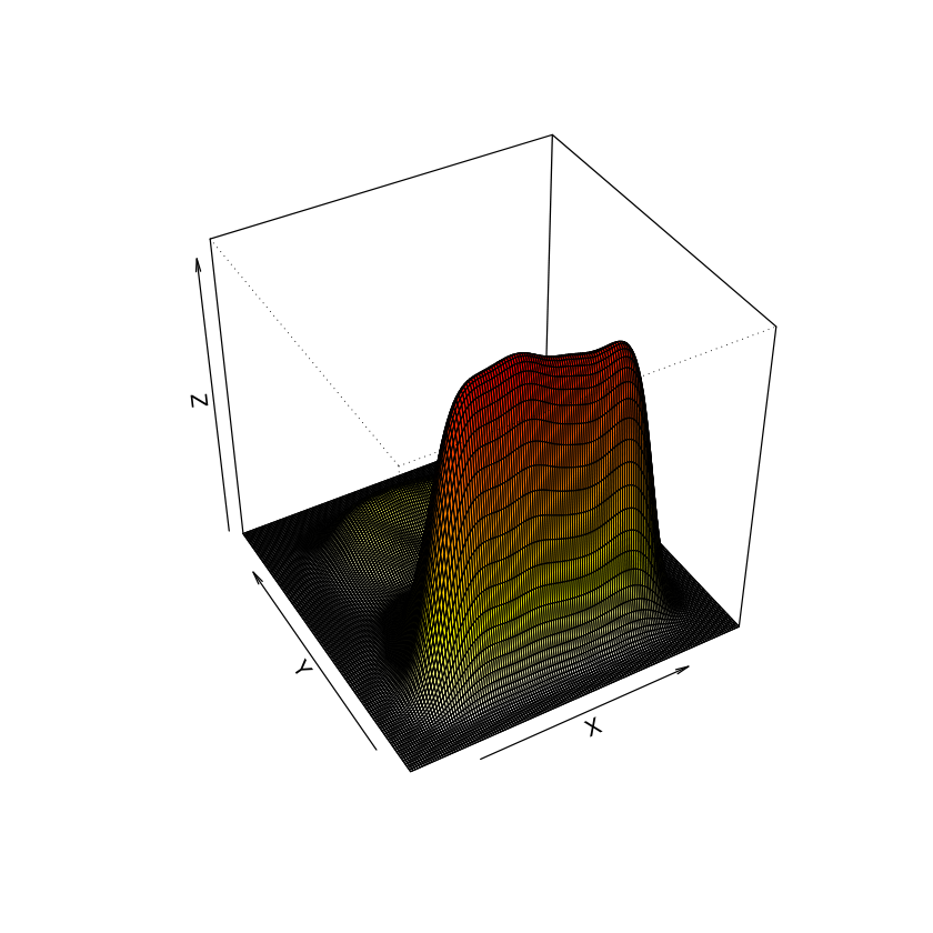
Figure 8 (a) shows the densities estimated by the LL-OPT and the FEE algorithms. As a comparison, kernel density estimated is in Figure 8 (b). We see that the uniformity in the first dimension of the distribution is well captured by OPT based approaches, but not by KDE.
 | |
| (a) | (b) |
Example 6.5.
We consider a 5-dimensional random vector
where are independent and sampled from
| (6.5) | |||
| (6.6) |
With a sample size of , the Hellinger distances for the LL-OPT and the FEE algorithms are 0.31 and 0.27, respectively. Figure 9 shows marginal histograms based on random samples drawn from the fitted FEE density and the true density. We can see that the fitted density resembles closely the true density in every dimension.
7 Discussion
We provide two software packages implementing the algorithms described in this paper, available at http://www.stanford.edu/group/wonglab/opt_comp/. The fast-opt package implements both the exact OPT and the LL-OPT algorithms described in Section 2 and 3. The smooth-opt package implements the smoothing algorithm described in Section 5. Both packages are implemented in C++.
The smooth-opt package relies on the user to specify the value for the tuning parameter . An alternative approach is to use cross-validation to choose which requires much more computation. In our simulations we found that the result is not sensitive to the value of and we use or in all our simulations.
High dimensional density estimation is a challenging task. The OPT is an adaptive non-parametric density estimation approach which fits to the global landscape of the data adaptively rather than locally as in kernel density estimation (Silverman, 1986), as demonstrated in our simulations. The simulations also suggest that our continuous piecewise linear FEE further improves upon the piecewise constant counterpart. The proposed FEE is a penalized regression approach. Based on a fast quadratic programming solver, it achieves decent efficiency when the sample size is reasonably high ( data points). The resulting estimated density function is continuous piecewise linear, which is mostly sufficient when we want to explore how the probability mass is distributed or visualize the estimated density. When necessary, the FEE can be extended to use higher order basis functions, at the cost of heavier computation.
Acknowledgements
This work was supported by NSF grant DMS-09-06044 and NIH grant R01-HG006018. We thank IBM® for providing the academic license of Cplex®.
References
- Akra and Bazzi [1998] M. Akra and L. Bazzi. On the solution of linear recurrence equations. Comput. Optim. Appl., 10(2):195–210, 1998.
- Allaire [2007] G. Allaire. Numerical Analysis and Optimization. Oxford Science Publications, 2007.
- Barron et al. [1992] A. R. Barron, L. Gyorfi, and E. C. van der Meulen. Distribution estimation consistent in total variation and in two types of information divergence. IEEE Trans. Inf. Theor., 38(5):1437–1454, 1992.
- Fan and Marron [1994] J. Fan and J. S. Marron. Fast implementations of nonparametric curve estimators. Journal of Computational and Graphical Statistics, page 35–56, 1994.
- Ferguson [1973] T. S. Ferguson. A Bayesian Analysis of Some Nonparametric Problems. The Annals of Statistics, 1(2):209–230, 1973.
- Ferguson [1974] T. S. Ferguson. Prior Distributions on Spaces of Probability Measures. The Annals of Statistics, 2(4):615–629, 1974.
- Gray [2003] A. G. Gray. Nonparametric density estimation: toward computational tractability. In In SIAM International Conference on Data Mining, 2003.
- Hastie et al. [2009] T. Hastie, R. Tibshirani, and J. H. Friedman. The Elements of Statistical Learning: Data Mining, Inference, and Prediction. Springer, 2nd edition, 2009.
- Jones et al. [1996] M. C. Jones, J. S. Marron, and S. J. Sheather. A brief survey of bandwidth selection for density estimation. Journal of the American Statistical Association, 91:401–407, 1996.
- Klemelä [2009] J. Klemelä. Smoothing of Multivariate Data: Density Estimation and Visualization. Wiley, 2009.
- Lugosi and Nobel [1996] G. Lugosi and A. Nobel. Consistency of data-driven histogram methods for density estimation and classification. Annals of Statistics, 24:687–706, 1996.
- Ma and Wong [2011] L. Ma and W. H. Wong. Coupling optional pólya trees and the two sample problem. Journal of the American Statistical Association, 106(496):1553–1565, 2011.
- Parzen [1962] E. Parzen. On Estimation of a Probability Density Function and Mode. The Annals of Mathematical Statistics, 33(3):1065–1076, 1962.
- Rosenblatt [1956] M. Rosenblatt. Remarks on some nonparametric estimates of a density function. The Annals of Mathematical Statistics, 27(3):832–837, 1956.
- Scott [1992] D. Scott. Multivariate Density Estimation: Theory, Practice and Visualization. Wiley, 1992.
- Scott [1979] D. W. Scott. On optimal and data-based histograms. Biometrika, 66(3):605–610, 1979.
- Silverman [1986] B. Silverman. Density estimation for statistics and data analysis. Monographs on statistics and applied probability. Chapman and Hall, 1986.
- Wand [1994] M. P. Wand. Fast computation of multivariate kernel estimators. Journal of Computational and Graphical Statistics, 3(4):433–445, 1994.
- Wong and Ma [2010] W. H. Wong and L. Ma. Optional Pólya tree and Bayesian inference. Ann. Stat., 38(3):1433–1459, 2010.
- Yang et al. [2003] C. Yang, R. Duraiswami, N. A. Gumerov, and L. Davis. Improved fast gauss transform and efficient kernel density estimation. In Proceedings of the Ninth IEEE International Conference on Computer Vision - Volume 2, 2003.