Off-shell helicity amplitudes in high-energy factorizationThanks: Presented at the Low x workshop, May 30 - June 4 2013, Rehovot and Eilat, Israel
Abstract
In the Catani-Ciafaloni-Hautmann high-energy factorization approach a cross section is expressed as a convolution of unintegrated gluon densities and a gauge-invariant hard process, in which two incoming gluons are off-shell with momenta satisfying certain high-energy kinematics. We present two methods of evaluating the tree-level hard process with multiple final states. The first one assumes that only one of the gluons is off-shell and relies on the Slavnov-Taylor identities. Such asymmetric configuration of incoming gluons is phenomenologically important in small x probing by forward processes. The second method deals also with two off-shell gluons and is based on the analytic continuation of the off-shell gluons momenta to the complex space. The methods were implemented into Monte Carlo computer programs and used in phenomenological applications. The results of both methods are straightforwardly related to Lipatov’s effective vertices in quasi-multi-regge kinematics.
1 Introduction
It is commonly known that in small x physics one needs a resummation of certain types of logarithms, that otherwise spoil the calculation. Such a procedure is provided by so-called high-energy factorization of Catani, Ciafaloni and Hautmann (CCH) [1, 2, 3, 4]. Its main ingredients are unintegrated gluon densities and off-shell matrix elements, which are the subject of the present talk. In general, only in simple cases an ordinary high-energy amplitude (i.e. evaluated from standard Feynman diagrams) can be gauge invariant despite its off-shellness. The CCH factorization was thus originally constructed for heavy quark production which is the exception just mentioned. At present, it is however highly desirable to use this approach to more complicated partonic final states.
One of the methods providing gauge invariant matrix elements that suits CCH approach is given in terms of the Lipatov’s effective action [5]. The resulting Feynman rules [6] involve (except standard QCD rules) additional so called induced vertices which possess complicated structure. Indeed, subsequent vertices with increasing number of legs have to be constructed recursively and explicit constructions exist up to five external legs [6]. For the recent applications of that approach in LHC phenomenology see e.g. [7, 8, 9, 10].
Let us point out, that the amplitudes we are talking about are merely tree-level amplitudes. In collinear approach (utilizing on-shell amplitudes) there are presently a lot of tools and methods allowing for automatic and efficient calculation of any tree-level process. This is certainly not the case for the off-shell amplitudes. Therefore two new method have been proposed in Refs. [11, 12]. The second method applies in certain, yet very important phenomenologically, situation of forward jet production processes. In what follows, after recalling the framework of high-energy factorization, we shall briefly describe the both methods.
2 High-energy factorization
A)
B)

The basic statement of CCH factorization is that at high energies, the cross section for the process for heavy quark hadroproduction can be expressed as
| (1) |
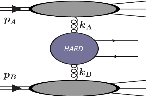
where , are hadrons with momenta , respectively, are unintegrated gluon densities undergoing the BFKL evolution and is the hard cross section for the process at tree level (Fig 1A ). The momenta of the off-shell gluons have the following high-energy form
| (2) |
where . The amplitude for the process is constructed using the ordinary diagram retaining however the gluon propagators and contracting them with eikonal vertices defined as and (Fig. 1B ). The amplitude is gauge invariant, fundamentally due to the form of the projectors.
In what follows we assume that the above factorization is still valid11 1 In the present short article we put aside comments about validity of -factorization at small x. We have gathered together some basic facts in [13], so we refer the reader to that paper and references therein. when replacing by any partonic state . The problem is, however, that simple generalization of the above prescription to calculate the hard matrix element does not lead to the gauge invariant result. As already mentioned in the Introduction additional contributions are needed. A general method to overcome this difficulty will be described in Section 3.
Let’s suppose now that we are interested in a situation where which occurs typically when one tries to access small x by looking at the forward jets. Since is large, one may assume that the gluon with momentum is nearly on-shell and transform the Eq. (1) into
| (3) |
where runs over gluon and all the quarks that can contribute to the production of multiparticle state (see also [14]). Now the hard process has a single leg off-shell, what somewhat simplifies the situation. A suitable method of evaluating such amplitudes will be outlined in Section 4.
3 The general method
Let us start with pointing out what are the features that we require from the new approach. First, it should use helicity method, which – generally speaking – is based on utilizing helicity spinors as a basic object used to construct the amplitudes. Second, it should be easily implementable in efficient computer programs, similar to the tools like HELAC for example [15].

A rather obvious attempt towards such an approach would be to embed the off-shell process into a bigger gauge invariant process as depicted in Fig. 2. It is however easy to see that it is impossible to maintain the on-shellness of all of the external partons and keep the momenta transfers and in the form of (2) in the same time. Obviously, compromising on-shellness of any of the quarks would spoil the gauge invariance. We may, however, as pointed out in [11], compromise real-valuedness of the momenta of the quarks. This will of course make the whole amplitude non-physical; the point is however that we are interested not in the quark amplitude, but rather in the off-shell amplitude.
To illustrate the method in some more details let us introduce four basis null vectors: real-valued , and complex-valued , defined as
| (4) |
where is a massles spinor corresponding to momentum and helicity (for more detail about helicity formalism see e.g. [16]). They satisfy and . The complex vectors , play the role of transverse vectors. Using this basis one may decompose the external quarks momenta as follows
| (5) | |||
| (6) |
where is a real parameter. Note, that this decomposition preserves both on-shellness and high-energy kinematics (2) for any . Another important property is that the spinors for external quarks satisfy the following proportionality relations , . Thus, we may trade the original spinors to the longitudinal spinors without spoiling the gauge invariance and thus simplifying the calculation. In order to decouple the unphysical (basically complex) degrees of freedom one has to take the smooth limit . In principle it can be done numerically, however the better solution is to do it analytically. Only external quark lines are directly affected by this limit and they turn out to be reduced to eikonal couplings and propagators, however in a fully controlled manner. The method was implemented in a MC code similar to HELAC and used to calculate certain distributions with four and five partons in the final state [11], what demonstrates its power.
4 One-leg off-shell amplitudes
As mentioned in Section 2, in small x practice one mostly needs the high-energy amplitudes with just a single gluon being off-shell. Of course the method described in the previous section applies here as well. Nevertheless, there is another interesting method [12] (predating the former) which we are now going to outline.
A)

B)
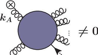
First, let us point out, that the CCH factorization is formulated in axial gauge. Thus, as a gauge invariant amplitudes we mean the ones that satisfy the Ward identities. To be more specific, let us denote the amplitude with off-shell leg and final state gluons as where are polarization vectors (Fig. 3A ). For a general choice of the amplitude does not satisfy the Ward identity (Fig. 3B )
| (7) |
The question that one can ask, is what is the actual value on the r.h.s. of (7) and whether one can use that information to construct a new amplitude
| (8) |
such that
| (9) |
The solution is provided by the basics of QCD, namely by the Slavnov-Taylor identities (see e.g. [17] for an elementary review). They however operate on the Green’s function level, therefore we need some sort of a reduction formula for high-energy factorization. It can be naturally written as
| (10) |
where is the momentum space Green’s function. The contraction of an external leg of with the corresponding momentum leads to gauge terms with ghost lines22 2 The fact that we use axial gauge for internal lines does not interfere with the usage of ghosts. Ghosts can be introduced in axial gauge, but they decouple from on-shell processes. (Fig. 4A ). After applying the reduction formula (10) the single term survives, which is precisely the r.h.s. of (7) (Fig. 4B ). Further, it turns out that by choosing the axial-gauge vector to be the “gauge-restoring amplitude” in (8) can be constructed by summing all the gauge contributions and trading the external ghosts for the longitudinal projections of polarization vectors. The result turns out to be very simple
| (11) |
where the subscript denotes that this result correspond to the specific color ordering of the external legs (the final answer is the sum of contributions for all color orderings). The case with quarks is actually very simple and does not require any “gauge-restoring amplitudes”, as can be seen by analyzing the Slavnov-Taylor identities. The above result allows for a very simple calculation of the pertinent amplitudes using the Berends-Giele recursion relations [18] and any polarization vectors. This method was implemented in the Monte Carlo program which uses FOAM algorithm [19].
A)

B)
5 Summary
We have presented the two methods of constructing gauge invariant off-shell amplitudes relevant to high-energy factorization. They correspond to Lipatov’s vertices in quasi-multi-regge kinematics. We have implemented the methods in the two independent Monte Carlo codes that allow to calculate the actual cross sections. Those tools have been recently [13] used to calculate the cross sections for three jet production at the LHC in the saturation regime using the unintegrated gluon densities from [20]. The method of Section 3 was recently extended in [21] to include off-shell quarks.
Acknowledgments
The author was supported by the NCBiR grant LIDER/02/35/L-2/10/NCBiR/2011.
References
- [1] S. Catani, M. Ciafaloni, and F. Hautmann, Nucl.Phys. B366, 135 (1991a)
- [2] S. Catani, M. Ciafaloni, and F. Hautmann, Nucl.Phys.Proc.Suppl. 18C, 220 (1991b)
- [3] S. Catani, M. Ciafaloni, and F. Hautmann, Phys.Lett. B242, 97 (1990)
- [4] S. Catani and F. Hautmann, Nucl.Phys. B427, 475 (1994), hep-ph/9405388
- [5] L. Lipatov, Nucl.Phys. B452, 369 (1995), hep-ph/9502308
- [6] E. Antonov, L. Lipatov, E. Kuraev, and I. Cherednikov, Nucl.Phys. B721, 111 (2005), hep-ph/0411185
- [7] M. Nefedov, V. Saleev, and A. V. Shipilova, Phys.Rev. D87, 094030 (2013), 1304.3549
- [8] V. Saleev and A. Shipilova, Phys.Rev. D86, 034032 (2012), 1201.4640
- [9] B. Kniehl, V. Saleev, A. Shipilova, and E. Yatsenko, Phys.Rev. D84, 074017 (2011), 1107.1462
- [10] M. Hentschinski and C. Salas, pp. 199–202 (2012), 1301.1227
- [11] A. van Hameren, P. Kotko, and K. Kutak, JHEP 1301, 078 (2013a), 1211.0961
- [12] A. van Hameren, P. Kotko, and K. Kutak, JHEP 1212, 029 (2012), 1207.3332
- [13] A. van Hameren, P. Kotko, and K. Kutak (2013b), 1308.0452
- [14] M. Deak, F. Hautmann, H. Jung, and K. Kutak, JHEP 0909, 121 (2009), 0908.0538
- [15] A. Cafarella, C. G. Papadopoulos, and M. Worek, Comput.Phys.Commun. 180, 1941 (2009), 0710.2427
- [16] M. L. Mangano and S. J. Parke, Phys.Rept. 200, 301 (1991), hep-th/0509223
- [17] H. Arodz and L. Hadasz, Lectures on Classical and Quantum Theory of Fields (Springer, 2010)
- [18] F. A. Berends and W. Giele, Nucl.Phys. B306, 759 (1988)
- [19] S. Jadach, Comput.Phys.Commun. 152, 55 (2003), physics/0203033
- [20] K. Kutak and S. Sapeta, Phys.Rev. D86, 094043 (2012), 1205.5035
- [21] A. van Hameren, K. Kutak, and T. Salwa (2013c), 1308.2861