A constructive approach to triangular trigonometric patches

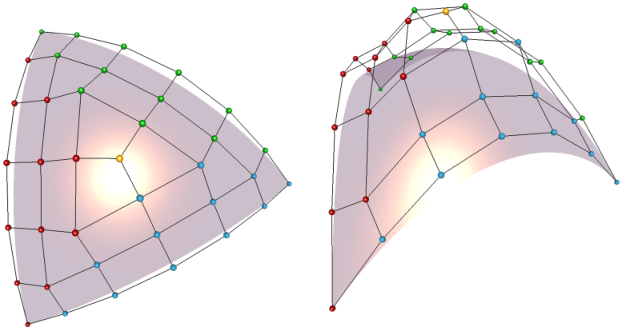
Ágoston Róth Email: agoston_roth@yahoo.com Address: Department of Mathematics and Computer Science, Babeş–Bolyai University, RO–400084 Cluj-Napoca, Romania Corresponding author: Corresponding author. Imre Juhász Address: Department of Descriptive Geometry, University of Miskolc, H-3515 Miskolc-Egyetemváros, Hungary Alexandru Kristály Address: Department of Economics, Babeş–Bolyai University, RO–400591 Cluj-Napoca, Romania

Abstract

We construct a constrained trivariate extension of the univariate normalized B-basis of the vector space of trigonometric polynomials of arbitrary (finite) order $n\in\mathbb{N}$ defined on any compact interval $\left[0,\alpha\right]$ , where $\alpha\in\left(0,\pi\right)$ . Our triangular extension is a normalized linearly independent constrained trivariate trigonometric function system of dimension $\delta_{n}=3n\left(n+1\right)+1$ that spans the same vector space of functions as the constrained trivariate extension of the canonical basis of truncated Fourier series of order $n$ over $\left[0,\alpha\right]$ . Although the explicit general basis transformation is yet unknown, the coincidence of these vector spaces is proved by means of an appropriate equivalence relation. As a possible application of our triangular extension, we introduce the notion of (rational) triangular trigonometric patches of order $n$ and of singularity free parametrization that could be used as control point based modeling tools in CAGD.

Keywords:

trigonometric polynomials, truncated Fourier series, constrained trivariate basis functions, triangular extension, triangular (rational) patches

1 Introduction

Triangular (rational) polynomial (spline) surfaces like the Coons [1], the Bernstein-Bézier [3, 2, 5] and the B-spline [4] triangular patches (and their rational variants) form an important aspect of CAGD. However, in order to provide control point based exact description of triangular parts of certain well-known surfaces, the rational form of these triangular patches should be used, which implies an undesired complexity (consider for example the evaluation of higher order (partial) derivatives, or the usage of non-negative special weights associated with control points that may be unknown for the designer) and in most cases provides a parametrization that does not reflect the variation of certain inner geometric properties (like curvature distribution) along the surface. One possibility to overcome some of these shortcomings is to consider the normalized B-basis of other (non-polynomial) vector spaces of functions that include the desired surfaces without the need of rational forms.

Non-polynomial surfaces like the first and second order triangular trigonometric patches and fourth order algebraic trigonometric ones were initiated by W.-Q. Shen, G.-Z. Wang and Y.-W. Wei in recent papers [9, 10] and [11], respectively. These special cases of triangular patches were obtained by certain constrained trivariate extensions of univariate normalized B-bases of the first and second order trigonometric and of the fourth order algebraic trigonometric vector spaces

	$\displaystyle\mathcal{F}_{2}^{\alpha}$	$\displaystyle=\operatorname{span}\left\{1,\cos\left(t\right),\sin\left(t\right):t\in\left[0,\alpha\right]\right\},$
	$\displaystyle\mathcal{F}_{4}^{\alpha}$	$\displaystyle=\operatorname{span}\left\{1,\cos\left(t\right),\sin\left(t\right),\cos\left(2t\right),\sin\left(2t\right):t\in\left[0,\alpha\right]\right\}$

and

\mathcal{M}_{4}^{\alpha}=\operatorname{span}\left\{1,t,\cos\left(t\right),\sin\left(t\right):t\in\left[0,\alpha\right]\right\},

respectively, where $\alpha\in\left(0,\pi\right)$ is an arbitrarily fixed shape (or design) parameter. The authors of the cited papers referred to their results as triangular Bernstein or Bézier-like (algebraic) trigonometric extensions and patches.

We restrict our attention only to the normalized B-basis of the vector space

\mathcal{F}_{2n}^{\alpha}=\operatorname{span}\left\{\cos\left(it\right),\sin\left(it\right):t\in\left[0,\alpha\right]\right\}_{i=0}^{n}

(1)

of truncated Fourier series (i.e., trigonometric polynomials of order at most $n\in\mathbb{N}$ ).

It was shown in [6] that vector space (1) has no normalized totally positive bases when $\alpha\geq\pi$ , i.e., in this case it does not provide shape preserving representations using control polygons. Thus, it is crucial for the shape parameter $\alpha$ to determine an interval of length strictly less than $\pi$ .

The normalized B-basis of the vector space (1) was introduced by J. Sánchez-Reyes in [8]. A linear reparametrization of his function system can be written in the form

\left\{A_{2n,i}^{\alpha}\left(t\right):t\in\left[0,\alpha\right]\right\}_{i=0}^{2n}=\left\{c_{2n,i}^{\alpha}\sin^{2n-i}\frac{\alpha-t}{2}\sin^{i}\frac{t}{2}:t\in\left[0,\alpha\right]\right\}_{i=0}^{2n},

(2)

where the normalizing non-negative coefficients

c_{2n,i}^{\alpha}=\frac{1}{\sin^{2n}\frac{\alpha}{2}}\sum_{r=0}^{\left\lfloor\frac{i}{2}\right\rfloor}\binom{n}{i-r}\binom{i-r}{r}\left(2\cos\frac{\alpha}{2}\right)^{i-2r},~i=0,1,\ldots,2n

fulfill the symmetry

c_{2n,i}^{\alpha}=c_{2n,2n-i}^{\alpha},~i=0,1,\ldots,n.

(3)

Our main objective is to construct the constrained trivariate counterpart of basis functions (2) over the triangular domain

\Omega^{\alpha}=\left\{\left(u,v,w\right)\in\left[0,\alpha\right]\times\left[0,\alpha\right]\times\left[0,\alpha\right]:u+v+w=\alpha\right\},

i.e., our intention is to propose a non-negative normalized basis for the constrained trivariate extension

\mathcal{V}_{n}^{\alpha}=\operatorname{span}V_{n}^{\alpha}

(4)

of the vector space (1), where the function system $V_{n}^{\alpha}$ consists of the largest linearly independent subset of the function system

\left\{\cos\left(ru+gv+bw\right),\sin\left(ru+gv+bw\right):\left(u,v,w\right)\in\Omega^{\alpha}\right\}_{r=0,g=0,b=0}^{n,n,n}.

Remark 1.1.

Note, that we only provide a special constrained trivariate extension of the univariate B-basis (2) that can be used to describe triangular (rational) trigonometric patches with boundary curves defined by linear combinations of control points and functions (2). We do not suggest that the proposed extension is also a B-basis. To the best of our knowledge, the notion of multivariate normalized B-basis (or something similar) does not even exist in the literature. The present paper describes some aspects of the proposed extension, but its global nature (e.g., whether its total behavior is similar to that of the multivariate Bernstein polynomials, or whether the multivariate Bernstein polynomials form the normalized B-basis of the vector space of multivariate polynomials of finite degree) needs further studies.

In CAGD, the expression constrained trivariate function system refers in fact to a bivariate one. Due to the constraint $u+v+w=\alpha$ each variable can be written as the linear combination of the remaining two independent ones. However, we do not fix which is pair assumed to be independent, since in most cases we will work with different parametrizations of the triangular domain $\Omega^{\alpha}$ .

As we already mentioned, the literature details only the special cases $n=1$ and $n=2$ in recent articles [9] and [10], respectively. In order to develop the general framework of the constrained trivariate extension of the univariate basis functions (2), we split our paper into eight sections that are outlined below.

Section 2 defines construction rules of a multiplicatively weighted oriented graph of $n\geq 1$ levels (numbered from $0$ to $n-1$ ) of nodes that store three groups of non-negative constrained trivariate trigonometric function systems (denoted by $R_{2n}^{\alpha}$ , $G_{2n}^{\alpha}$ and $B_{2n}^{\alpha}$ ) of order $n$ over $\Omega^{\alpha}$ that fulfill six cyclic symmetry properties in their variables. The union $T_{2n}^{\alpha}$ of these function systems will form the basis of the constrained trivariate extension of univariate basis functions (2).

The linear independence of $T_{2n}^{\alpha}$ will be proved in Section 3 by exploiting the symmetry properties of the oriented graph. More precisely, using three periodically rotating parametrizations of $\Omega^{\alpha}$ , we apply a technique based on a special form of mathematical induction on the order of partial derivatives of a vanishing linear combination of constrained trivariate functions $R_{2n}^{\alpha}$ , $G_{2n}^{\alpha}$ and $B_{2n}^{\alpha}$ .

Section 4 introduces an equivalence relation by means of which one can recursively construct the linearly independent function system $V_{n}^{\alpha}$ that spans the constrained trivariate extension $\mathcal{V}_{n}^{\alpha}$ of the univariate vector space $\mathcal{F}_{2n}^{\alpha}$ . As expected, vector spaces $\mathcal{T}_{2n}^{\alpha}=\operatorname{span}T_{2n}^{\alpha}$ and $\mathcal{V}_{n}^{\alpha}=\operatorname{span}V_{n}^{\alpha}$ coincide. Indeed, using equivalence classes we also prove the latter statement along with the determination of the common dimension $\delta_{n}=3n\left(n+1\right)+1$ of these vector spaces.

Section 5 offers a procedure to obtain the normalized form $\overline{T}_{2n}^{\alpha}$ of the function system $T_{2n}^{\alpha}$ . Due to the complexity of this problem, closed formulas of corresponding non-negative, symmetric and unique normalizing coefficients are given only in case of levels $0$ and $1$ for arbitrary order, and for all levels just for orders $n=1$ , $2$ and $3$ .

Section 6 lists possible applications of our constrained triangular extension by providing control point based surface modeling tools that may be used in CAGD. Subsection 6.1 introduces the notion of triangular trigonometric patches of order $n$ and presents some of their geometric properties. Using non-negative weights of rank $1$ and quotient basis functions, the rational counterpart of $\overline{T}_{2n}^{\alpha}$ is formulated in Subsection 6.2 that defines triangular rational trigonometric patches.

Compared to the classical constrained trivariate Bernstein polynomials on triangular domains, in this non-polynomial case, theoretical questions are significantly harder to answer even for special values of the order $n$ . Since we cannot answer some theoretical questions in their full generality for the present, Section 7 formulates several open problems like the general basis transformation between vector spaces $\mathcal{T}_{2n}^{\alpha}$ and $\mathcal{V}_{n}^{\alpha}$ , the non-negativity, symmetry properties and closed/recursive formulas of normalizing coefficients of arbitrary order, general order elevation, and convergence of (rational) triangular trigonometric patches to (rational) Bézier triangles when $\alpha\to 0$ .

Remark 1.2 (Technical report).

In order to reduce the length of the paper, technical details of some proofs and reformulations are left out, that can be found in the technical report [7].

2 Constrained trivariate function systems $R_{2n}^{\alpha}$ , $G_{2n}^{\alpha}$ and $B_{2n}^{\alpha}$ : a graph-based approach

Consider the oriented graph of order $n\geq 1$ illustrated in Fig. 1(a).

Figure 1: (a) Construction rules of constrained trivariate function systems (5), (6) and (7). (b) The red, green and blue domains correspond to systems (5), (6) and (7), respectively. Functions associated with the red, green and blue shaded domains are symmetric in variables

\left(w,u\right)

\left(v,w\right)

and

\left(u,v\right)

, respectively. Functions which correspond to the adjacent domains red–green, green–blue and blue–red are symmetric in variables

\left(v,u\right)

\left(u,w\right)

and

\left(w,v\right)

, respectively. (For interpretation of the references to color in this figure legend, the reader is referred to the web version of this paper.)

The three outermost nodes (i.e., the vertices of the outermost triangle) store the functions $\sin^{2n}\frac{u}{2}$ , $\sin^{2n}\frac{v}{2}$ and $\sin^{2n}\frac{w}{2}$ . Each directed edge has a weight function that defines a multiplication factor when one follows a path from a given node to another one. Tracking a given path and multiplying by weight functions along the edges, determines the function stored in an inner node of the graph. Observe that the layout of these multiplicative weight functions ensures that all paths starting from an outermost node and terminating at the innermost one (i.e., the common centroid of triangles) generate the same constrained trivariate function $\sin^{n}\frac{u}{2}\sin^{n}\frac{v}{2}\sin^{n}\frac{w}{2}$ . Based on these multiplication rules, one can introduce the constrained trivariate function systems

	$\displaystyle R_{2n}^{\alpha}$	$\displaystyle=\left\{R_{2n,2n-i,j}^{\alpha}\left(u,v,w\right):\left(u,v,w\right)\in\Omega^{\alpha}\right\}_{j=0,i=j}^{n,2n-j},$		(5)
	$\displaystyle G_{2n}^{\alpha}$	$\displaystyle=\left\{G_{2n,2n-i,j}^{\alpha}\left(u,v,w\right):\left(u,v,w\right)\in\Omega^{\alpha}\right\}_{j=0,i=j}^{n,2n-j}$		(6)

and

B_{2n}^{\alpha}=\left\{B_{2n,2n-i,j}^{\alpha}\left(u,v,w\right):\left(u,v,w\right)\in\Omega^{\alpha}\right\}_{j=0,i=j}^{n,2n-j},

(7)

where

$\displaystyle\left\{R_{2n,2n-i,j}^{\alpha}\left(u,v,w\right)\right\}_{j=0,i=j}^{n,n}$	$\displaystyle=\left\{\sin^{2n-i}\frac{u}{2}\sin^{i}\frac{w}{2}\cos^{i-j}\frac{v}{2}\sin^{j}\frac{v}{2}\right\}_{j=0,i=j}^{n,n},$	(8)

$\displaystyle\left\{R_{2n,2n-i,j}^{\alpha}\left(u,v,w\right)\right\}_{j=0,i=n+1}^{n-1,2n-j}$	$\displaystyle=\left\{R_{2n,i,j}^{\alpha}\left(w,v,u\right)\right\}_{j=0,i=n+1}^{n-1,2n-j}$	(9)
	$\displaystyle=\left\{\sin^{i}\frac{w}{2}\sin^{2n-i}\frac{u}{2}\cos^{2n-i-j}\frac{v}{2}\sin^{j}\frac{v}{2}\right\}_{j=0,i=n+1}^{n-1,2n-j},$

and due to the symmetry

$\displaystyle\left\{G_{2n,2n-i,j}^{\alpha}\left(u,v,w\right)\right\}_{j=0,i=j}^{n,n}$	$\displaystyle=\left\{R_{2n,2n-i,j}^{\alpha}\left(w,u,v\right)\right\}_{j=0,i=j}^{n,n}$	(10)
	$\displaystyle=\left\{\sin^{2n-i}\frac{w}{2}\sin^{i}\frac{v}{2}\cos^{i-j}\frac{u}{2}\sin^{j}\frac{u}{2}\right\}_{j=0,i=j}^{n,n},$

$\displaystyle\left\{G_{2n,2n-i,j}^{\alpha}\left(u,v,w\right)\right\}_{j=0,i=n+1}^{n-1,2n-j}$	$\displaystyle=\left\{G_{2n,i,j}^{\alpha}\left(u,w,v\right)\right\}_{j=0,i=n+1}^{n-1,2n-j}$	(11)
	$\displaystyle=\left\{\sin^{i}\frac{v}{2}\sin^{2n-i}\frac{w}{2}\cos^{2n-i-j}\frac{u}{2}\sin^{j}\frac{u}{2}\right\}_{j=0,i=n+1}^{n-1,2n-j},$

$\displaystyle\left\{B_{2n,2n-i,j}^{\alpha}\left(u,v,w\right)\right\}_{j=0,i=j}^{n,n}$	$\displaystyle=\left\{R_{2n,2n-i,j}^{\alpha}\left(v,w,u\right)\right\}_{j=0,i=j}^{n,n}$	(12)
	$\displaystyle=\left\{\sin^{2n-i}\frac{v}{2}\sin^{i}\frac{u}{2}\cos^{i-j}\frac{w}{2}\sin^{j}\frac{w}{2}\right\}_{j=0,i=j}^{n,n},$

$\displaystyle\left\{B_{2n,2n-i,j}^{\alpha}\left(u,v,w\right)\right\}_{j=0,i=n+1}^{n-1,2n-j}$	$\displaystyle=\left\{B_{2n,i,j}^{\alpha}\left(v,u,w\right)\right\}_{j=0,i=n+1}^{n-1,2n-j}$	(13)
	$\displaystyle=\left\{\sin^{i}\frac{u}{2}\sin^{2n-i}\frac{v}{2}\cos^{2n-i-j}\frac{w}{2}\sin^{j}\frac{w}{2}\right\}_{j=0,i=n+1}^{n-1,2n-j}.$

Observe that function systems (5), (6) and (7) consist of non-negative functions which fulfill the six symmetry properties illustrated in Fig. 1(b).

In what follows, we study the properties of the constrained trivariate non-negative joint function system

\begin{array}[c]{ccl}T_{2n}^{\alpha}&=&\left\{R_{2n,2n-i,j}^{\alpha}\left(u,v,w\right),G_{2n,2n-i,j}^{\alpha}\left(u,v,w\right),B_{2n,2n-i,j}^{\alpha}\left(u,v,w\right):\left(u,v,w\right)\in\Omega^{\alpha}\right\}_{j=0,i=j}^{n-1,2n-1-j}\\ &&\\ &&\cup\left\{R_{2n,n,n}^{\alpha}\left(u,v,w\right)=G_{2n,n,n}^{\alpha}\left(u,v,w\right)=B_{2n,n,n}^{\alpha}\left(u,v,w\right):\left(u,v,w\right)\in\Omega^{\alpha}\right\}\end{array}

(14)

of order $n\geq 1$ . We refer to the index $j$ of these functions as levels since they correspond to the nested triangles shrinking from the boundary to their common centroid depicted in Fig. 1(a). Fig. 2 illustrates the layout of the constrained trivariate function system $T_{6}^{\alpha}$ of order $3$ .

Figure 2: The layout of the constrained trivariate joint function system (14) of order

n=3

Note that the function system (14) is reduced to the univariate B-basis (2) whenever one of the three variables $u$ , $v$ and $w$ vanishes, i.e., the system fulfills the boundary properties

$\displaystyle\left.T_{2n}^{\alpha}\right\|_{v=0}$	$\displaystyle=\left\{\frac{1}{c_{2n,2n-i}^{\alpha}}A_{2n,2n-i}^{\alpha}\left(u\right):u\in\left[0,\alpha\right]\right\}_{i=0}^{2n},$	(15)
$\displaystyle\left.T_{2n}^{\alpha}\right\|_{u=0}$	$\displaystyle=\left\{\frac{1}{c_{2n,2n-i}^{\alpha}}A_{2n,2n-i}^{\alpha}\left(w\right):w\in\left[0,\alpha\right]\right\}_{i=0}^{2n},$	(16)
$\displaystyle\left.T_{2n}^{\alpha}\right\|_{w=0}$	$\displaystyle=\left\{\frac{1}{c_{2n,2n-i}^{\alpha}}A_{2n,2n-i}^{\alpha}\left(v\right):v\in\left[0,\alpha\right]\right\}_{i=0}^{2n}.$	(17)

Proposition 2.1 (Bernstein polynomials of degree $2n$ as special case).

If one uses the linear reparametrization $t\left(s\right)=\alpha s,~s\in\left[0,1\right]$ , then basis functions (2) of order $n$ converge to the Bernstein polynomials of degree $2n$ when $\alpha\rightarrow 0$ , i.e.,

\lim_{\alpha\rightarrow 0}A_{2n,i}^{\alpha}\left(\alpha s\right)=B_{i}^{2n}\left(s\right),\,\forall s\in\left[0,1\right],~i=0,1,\ldots,2n\text{.}

(18)

Proof.

In Reference [8] functions (2) were obtained by raising the identity

A_{2n,0}^{\alpha}\left(\alpha s\right)+A_{2n,1}^{\alpha}\left(\alpha s\right)+A_{2n,2}^{\alpha}\left(\alpha s\right)=1,~\forall s\in\left[0,1\right]

to the power $n$ , i.e.,

\sum_{i=0}^{2n}A_{2n,i}^{\alpha}\left(\alpha s\right)=\left(A_{2n,0}^{\alpha}\left(s\right)+A_{2n,1}^{\alpha}\left(s\right)+A_{2n,2}^{\alpha}\left(s\right)\right)^{n}=1,~\forall s\in\left[0,1\right]

which in the limiting case $\alpha\rightarrow 0$ takes the form

		$\displaystyle\lim_{\alpha\rightarrow 0}\left(\frac{1}{\sin^{2}\left(\frac{\alpha}{2}\right)}\sin^{2}\left(\frac{\alpha-\alpha s}{2}\right)+\frac{2\cos\left(\frac{\alpha}{2}\right)}{\sin^{2}\left(\frac{\alpha}{2}\right)}\sin\left(\frac{\alpha-\alpha s}{2}\right)\sin\left(\frac{\alpha s}{2}\right)+\frac{1}{\sin^{2}\left(\frac{\alpha}{2}\right)}\sin^{2}\left(\frac{\alpha s}{2}\right)\right)^{n}$
	$\displaystyle=$	$\displaystyle\left(\left(1-s\right)^{2}+2\left(1-s\right)s+s^{2}\right)^{n}$
	$\displaystyle=$	$\displaystyle\left(\left(1-s\right)+s\right)^{2n}$
	$\displaystyle=$	$\displaystyle\sum_{i=0}^{2n}B_{i}^{2n}\left(s\right)$

for all values of $s\in\left[0,1\right]$ , since $\lim\limits_{\alpha\rightarrow 0}\frac{\sin\left(\frac{\alpha s}{2}\right)}{\sin\left(\frac{\alpha}{2}\right)}=s$ and $\lim\limits_{\alpha\rightarrow 0}\cos\left(\frac{\alpha s}{2}\right)=1.$ ∎

3 Linear independence

The linear independence of the joint function system (14) will be proved by using higher order mixed partial derivatives. In order to evaluate these derivates, when one of the constrained variables equals $0$ , we have to study the behavior of functions

	$\displaystyle C_{i,\lambda}^{p}\left(t\right)$	$\displaystyle=\frac{\text{d}^{p}}{\text{d}t^{p}}\cos^{i}\left(\lambda t\right),~t\in\mathbb{R},$
	$\displaystyle S_{j,\mu}^{p}\left(t\right)$	$\displaystyle=\frac{\text{d}^{p}}{\text{d}t^{p}}\sin^{j}\left(\mu t\right),~t\in\mathbb{R}$

and

M_{i,\lambda,j,\mu}^{z}\left(t\right)=\frac{\text{d}^{z}}{\text{d}t^{z}}\left(\cos^{i}\left(\lambda t\right)\sin^{j}\left(\mu t\right)\right)

at $t=0$ , where exponents $i$ , $j$ and orders $p$ , $z$ are natural numbers, while angular velocities $\lambda,\mu>0$ are real parameters. The proofs of the following Lemma 3.1 and Proposition 3.1 can be found in [7].

Lemma 3.1.

Let $i$ , $j$ and $p$ be natural numbers greater than or equal to $1$ . If $\lambda,\mu>0$ , then signs of values $\left\{C_{i,\lambda}^{p}\left(0\right)\right\}_{p\geq 0}$ and $\left\{S_{j,\mu}^{p}\left(0\right)\right\}_{p\geq 0}$ are

\operatorname{sign}C_{i,\lambda}^{p}\left(0\right)=\left\{\begin{array}[c]{rl}-1,&~p-i=2r,~r\equiv 1\left(\operatorname{mod}2\right),\\ 0,&~p\equiv 1\left(\operatorname{mod}2\right),\\ +1,&~p-i=2r,~r\equiv 0\left(\operatorname{mod}2\right)\end{array}\right.

(19)

and

\operatorname{sign}S_{j,\mu}^{p}\left(0\right)=\left\{\begin{array}[c]{rl}-1,&~p\geq j,~p-j=2r,~r\equiv 1\left(\operatorname{mod}2\right),\\ 0,&~\left(p<j\right)\ \text{or }\left(p-j\equiv 1\left(\operatorname{mod}2\right)\text{ and }p>j\right),\\ +1,&~p\geq j,~p-j=2r,~r\equiv 0\left(\operatorname{mod}2\right),\end{array}\right.

(20)

respectively. (In particular, $S_{j,\mu}^{j}\left(0\right)=j!\mu^{j}$ ).

Proposition 3.1.

Independently of $i\in\mathbb{N}$ and $\lambda,\mu>0$ , for all values of $j,z\in\mathbb{N}$ such that $i+j\neq 0$ and $z\geq 1$ we have the equality

\operatorname{sign}M_{i,\lambda,j,\mu}^{z}\left(0\right)=\left\{\begin{array}[c]{rl}-1,&~z-j\equiv 2\left(\operatorname{mod}4\right)\text{ and }z\geq j,\\ 0,&~\left(z<j\right)\text{ or }\left(z-j\equiv\pm 1\left(\operatorname{mod}4\right)\text{ and }z>j\right),\\ +1,&~z-j\equiv 0\left(\operatorname{mod}4\right)\text{ and }z\geq j.\end{array}\right.

(21)

Under the parametrization

\left\{\begin{array}[c]{rcl}u\left(x,y\right)&=&\alpha-x,~x\in\left[0,\alpha\right],\\ v\left(x,y\right)&=&y,~y\in\left[0,\alpha-x\right],\\ w\left(x,y\right)&=&x-y,\end{array}\right.

(22)

of $\Omega^{\alpha}$ , one can easily show that the $r$ th order ( $r\geq 0$ ) partial derivative of any smooth function $L:\Omega^{\alpha}\rightarrow\mathbb{R}$ with respect to the variable $y$ is

\frac{\partial^{r}}{\partial y^{r}}L\left(u\left(x,y\right),v\left(x,y\right),w\left(x,y\right)\right)=\sum_{k=0}^{r}\dbinom{r}{k}\left(-1\right)^{k}\frac{\partial^{r}}{\partial v^{r-k}\partial w^{k}}L\left(u\left(x,y\right),v\left(x,y\right),w\left(x,y\right)\right).

(23)

If the function $L$ is defined as the linear combination

\begin{array}[c]{ccl}L\left(u,v,w\right)&=&\rho_{2n,n,n}R_{2n,n,n}^{\alpha}\left(u,v,w\right)+{\displaystyle\sum\limits_{j=0}^{n-1}}{\displaystyle\sum\limits_{i=j}^{2n-1-j}}\rho_{2n,2n-i,j}R_{2n,2n-i,j}^{\alpha}\left(u,v,w\right)\\ &&+{\displaystyle\sum\limits_{j=0}^{n-1}}{\displaystyle\sum\limits_{i=j}^{2n-1-j}}\gamma_{2n,2n-i,j}G_{2n,2n-i,j}^{\alpha}\left(u,v,w\right)+{\displaystyle\sum\limits_{j=0}^{n-1}}{\displaystyle\sum\limits_{i=j}^{2n-1-j}}\beta_{2n,2n-i,j}B_{2n,2n-i,j}^{\alpha}\left(u,v,w\right)\end{array}

(24)

where $\rho_{2n,n,n}$ , $\left\{\rho_{2n,2n-i,j}\right\}_{j=0,i=j}^{n-1,2n-1-j}$ , $\left\{\gamma_{2n,2n-i,j}\right\}_{j=0,i=j}^{n-1,2n-1-j}$ and $\left\{\beta_{2n,2n-i,j}\right\}_{j=0,i=j}^{n-1,2n-1-j}$ are real scalars, then, by the help of Proposition 3.1, one can easily determine those functions of system (14) the higher order mixed partial derivatives ( $\frac{\partial^{r}}{\partial v^{r-k}\partial w^{k}}\left(\cdot\right)$ , $k=0,1,\ldots,r$ ) of which vanish when one evaluates the terms of (23) at $y=0$ . In the case of $n=4$ , we have provided an example in Fig. 3.

Figure 3: (a)–(e) Using the sign function (21), one can easily verify that black and non-black dots represent those functions of system (14) the

4

th order mixed partial derivatives of which with respect to

v\left(x,y\right)=y

and

w\left(x,y\right)=x-y

are zero and non-zero, respectively, under parametrization (22) at

y=0

. Observe, that the gray shaded areas correspond to functions which comprise the factor

\sin\frac{v\left(x,y\right)}{2}=\sin\frac{y}{2}

raised to a power greater than the corresponding order

k=0,1,\ldots,4

of the partial derivative with respect to

v\left(x,y\right)=y

. Thus, these partial derivatives vanish at

y=0

due to the first condition of the zero branch of the sign function (21). Black dots that fall outside of the gray shaded areas correspond to constrained trivariate functions that comprise the factor

\sin\frac{v\left(x,y\right)}{2}=\sin\frac{y}{2}

raised to a power which – together with the order

k=0,1,\ldots,4

of the partial derivative with respect to

v\left(x,y\right)=y

, at

y=0

– fulfills the second condition of the zero branch of the sign function (21). (For interpretation of the references to color in this figure legend, the reader is referred to the web version of this paper.)

Theorem 3.1 (Linear independence of the joint systems).

The function system (14) is linearly independent and the dimension of the vector space $\mathcal{T}_{2n}^{\alpha}=~$ span $\emph{~}T_{2n}^{\alpha}$ is

\delta_{n}=3n\left(n+1\right)+1.

Proof.

It is easy to verify that the number of functions in system (14) is exactly

\delta_{n}=1+3\sum_{j=0}^{n-1}\sum_{i=j}^{2n-1-j}1=1+3n\left(n+1\right).

Consider the linear combination (24) and assume that the equality

L\left(u,v,w\right)=0

(25)

holds for all $\left(u,v,w\right)\in\Omega^{\alpha}$ .

If equality (25) holds for all $\left(u,v,w\right)\in\Omega^{\alpha}$ then it is also valid under all possible parametrizations of the definition domain $\Omega^{\alpha}$ . In what follows, we will work with three different parametrizations of $\Omega^{\alpha}$ , namely with

\left\{\begin{array}[c]{rcl}u_{1}\left(x,y\right)&=&x,~x\in\left[0,\alpha\right],\\ v_{1}\left(x,y\right)&=&y,~y\in\left[0,\alpha-x\right],\\ w_{1}\left(x,y\right)&=&\alpha-x-y,\end{array}\right.

(26)

\left\{\begin{array}[c]{rcl}u_{2}\left(x,y\right)&=&x,~x\in\left[0,\alpha\right],\\ v_{2}\left(x,y\right)&=&\alpha-x-y,\\ w_{2}\left(x,y\right)&=&y,~y\in\left[0,\alpha-x\right],\end{array}\right.

(27)

and

\left\{\begin{array}[c]{rcl}u_{3}\left(x,y\right)&=&\alpha-x-y,\\ v_{3}\left(x,y\right)&=&x,~x\in\left[0,\alpha\right],\\ w_{3}\left(x,y\right)&=&y,~y\in\left[0,\alpha-x\right].\end{array}\right.

(28)

Straight calculations show that

$\displaystyle\frac{\partial^{r}}{\partial y^{r}}L\left(u_{1}\left(x,y\right),v_{1}\left(x,y\right),w_{1}\left(x,y\right)\right)$	$\displaystyle=\sum_{k=0}^{r}\dbinom{r}{k}\left(-1\right)^{k}\frac{\partial^{r}}{\partial v_{1}^{r-k}\partial w_{1}^{k}}L\left(u_{1}\left(x,y\right),v_{1}\left(x,y\right),w_{1}\left(x,y\right)\right),$	(29)

$\displaystyle\frac{\partial^{r}}{\partial x^{r}}L\left(u_{2}\left(x,y\right),v_{2}\left(x,y\right),w_{2}\left(x,y\right)\right)$	$\displaystyle=\sum_{k=0}^{r}\dbinom{r}{k}\left(-1\right)^{k}\frac{\partial^{r}}{\partial u_{2}^{r-k}\partial v_{2}^{k}}L\left(u_{2}\left(x,y\right),v_{2}\left(x,y\right),w_{2}\left(x,y\right)\right),$	(30)

$\displaystyle\frac{\partial^{r}}{\partial y^{r}}L\left(u_{3}\left(x,y\right),v_{3}\left(x,y\right),w_{3}\left(x,y\right)\right)$	$\displaystyle=\sum_{k=0}^{r}\dbinom{r}{k}\left(-1\right)^{k}\frac{\partial^{r}}{\partial w_{3}^{r-k}\partial u_{3}^{k}}L\left(u_{3}\left(x,y\right),v_{3}\left(x,y\right),w_{3}\left(x,y\right)\right)$	(31)

for all $x\in\left[0,\alpha\right]$ , $\ y\in\left[0,\alpha-x\right]$ and order $r\in\mathbb{N}$ .

In order to prove the statement, we argue by mathematical induction on the derivation order $r=0,1,\ldots,n$ .

In the case of $r=0$ and parametrization (26), observe that at $y=0$ equality (25) becomes

	$\displaystyle 0$	$\displaystyle=\left.L\left(u_{1}\left(x,y\right),v_{1}\left(x,y\right),w_{1}\left(x,y\right)\right)\right\|_{y=0}$
		$\displaystyle=\sum_{i=0}^{2n-1}\rho_{2n,2n-i,0}R_{2n,2n-i,0}^{\alpha}\left(x,0,\alpha-x\right)+\gamma_{2n,2n,0}G_{2n,2n,0}^{\alpha}\left(x,0,\alpha-x\right)$
		$\displaystyle=\sum_{i=0}^{2n-1}\rho_{2n,2n-i,0}\sin^{2n-i}\frac{x}{2}\sin^{i}\frac{\alpha-x}{2}+\gamma_{2n,2n-i,0}\sin^{2n}\frac{\alpha-x}{2}$
		$\displaystyle=\sum_{i=0}^{2n}\rho_{2n,2n-i,0}^{\prime}c_{2n,2n-i}^{\alpha}\sin^{2n-i}\frac{x}{2}\sin^{i}\frac{\alpha-x}{2}$
		$\displaystyle=\sum_{i=0}^{2n}\rho_{2n,2n-i,0}^{\prime}A_{2n,2n-i}^{\alpha}\left(x\right),~\forall x\in\left[0,\alpha\right],$

where we have used the notation

\rho_{2n,2n-i,0}^{\prime}=\left\{\begin{array}[c]{rl}\dfrac{\rho_{2n,2n-i,0}}{c_{2n,2n-i}^{\alpha}},&i=0,1,\ldots,2n-1,\\ &\\ \dfrac{\gamma_{2n,2n,0}}{c_{2n,0}^{\alpha}},&i=2n\end{array}\right.

and the fact that all omitted functions include the factor $\left.\sin\frac{v_{1}\left(x,y\right)}{2}\right|_{y=0}=\left.\sin\frac{y}{2}\right|_{y=0}=0$ raised to a power at least one. Since the function system $\left\{A_{2n,2n-i}^{\alpha}\left(x\right):x\in\left[0,\alpha\right]\right\}_{i=0}^{2n}$ is linearly independent, it follows that

\rho_{2n,2n-i,0}^{\prime}=0,~i=0,1,\ldots,2n.

Thus, equality (25) can be reduced to

\begin{array}[c]{ccl}0&=&\widetilde{L}\left(u,v,w\right)\\ &=&\rho_{2n,n,n}R_{2n,n,n}^{\alpha}\left(u,v,w\right)+{\displaystyle\sum\limits_{j=1}^{n-1}}{\displaystyle\sum\limits_{i=j}^{2n-1-j}}\rho_{2n,2n-i,j}R_{2n,2n-i,j}^{\alpha}\left(u,v,w\right)\\ &&+{\displaystyle\sum\limits_{i=1}^{2n-1}}\gamma_{2n,2n-i,0}G_{2n,2n-i,0}^{\alpha}\left(u,v,w\right)+{\displaystyle\sum\limits_{j=1}^{n-1}}{\displaystyle\sum\limits_{i=j}^{2n-1-j}}\gamma_{2n,2n-i,j}G_{2n,2n-i,j}^{\alpha}\left(u,v,w\right)\\ &&+{\displaystyle\sum\limits_{j=0}^{n-1}}{\displaystyle\sum\limits_{i=j}^{2n-1-j}}\beta_{2n,2n-i,j}B_{2n,2n-i,j}^{\alpha}\left(u,v,w\right),~\forall\left(u,v,w\right)\in\Omega^{\alpha}.\end{array}

(32)

Now, considering parametrization (27) and the partial derivative of order $r=0$ of equality (32) with respect to the variable $x$ , at $x=0$ , we obtain that

	$\displaystyle 0$	$\displaystyle=\left.\widetilde{L}\left(u_{2}\left(x,y\right),v_{2}\left(x,y\right),w_{2}\left(x,y\right)\right)\right\|_{x=0}$
		$\displaystyle=\sum_{i=1}^{2n-1}\gamma_{2n,2n-i,0}G_{2n,2n-i,0}^{\alpha}\left(0,\alpha-y,y\right)+\beta_{2n,2n,0}B_{2n,2n,0}^{\alpha}\left(0,\alpha-y,y\right)$
		$\displaystyle=\sum_{i=1}^{2n}\gamma_{2n,2n-i,0}^{\prime}A_{2n,2n-i}^{\alpha}\left(y\right),~\forall y\in\left[0,\alpha\right],$

where we have used the notation

\gamma_{2n,2n-i,0}^{\prime}=\left\{\begin{array}[c]{rl}\dfrac{\gamma_{2n,2n-i,0}}{c_{2n,2n-i}^{\alpha}},&i=1,2,\ldots,2n-1,\\ &\\ \dfrac{\beta_{2n,2n,0}}{c_{2n,0}^{\alpha}},&i=2n\end{array}\right.

and the fact that discarded functions include the factor $\left.\sin\frac{u_{2}\left(x,y\right)}{2}\right|_{x=0}=\left.\sin\frac{x}{2}\right|_{x=0}=0$ raised to a power greater than or equal to one. Due to the linear independence of the univariate function system $\left\{A_{2n,2n-i}^{\alpha}\left(y\right):y\in\left[0,\alpha\right]\right\}_{i=1}^{2n}$ , one has that

\gamma_{2n,2n-i,0}^{\prime}=0,~i=1,2,\ldots,2n.

Therefore, equality (32) can be simplified to the form

\begin{array}[c]{rll}0&=&\widehat{L}\left(u,v,w\right)\\ &=&\rho_{2n,n,n}R_{2n,n,n}^{\alpha}\left(u,v,w\right)+{\displaystyle\sum\limits_{j=1}^{n-1}}{\displaystyle\sum\limits_{i=j}^{2n-1-j}}\rho_{2n,2n-i,j}R_{2n,2n-i,j}^{\alpha}\left(u,v,w\right)\\ &&+{\displaystyle\sum\limits_{j=1}^{n-1}}{\displaystyle\sum\limits_{i=j}^{2n-1-j}}\gamma_{2n,2n-i,j}G_{2n,2n-i,j}^{\alpha}\left(u,v,w\right)\\ &&+{\displaystyle\sum\limits_{i=1}^{2n-1}}\beta_{2n,2n-i,0}B_{2n,2n-i,0}^{\alpha}\left(u,v,w\right)+{\displaystyle\sum\limits_{j=1}^{n-1}}{\displaystyle\sum\limits_{i=j}^{2n-1-j}}\beta_{2n,2n-i,j}B_{2n,2n-i,j}^{\alpha}\left(u,v,w\right),~\forall\left(u,v,w\right)\in\Omega^{\alpha}.\end{array}

(33)

Performing similar calculations as above, but using parametrization (28) and the zeroth order partial derivative of equality (33) with respect to $y$ , at $y=0$ , we obtain that

	$\displaystyle 0$	$\displaystyle=\left.\widehat{L}\left(u_{3}\left(x,y\right),v_{3}\left(x,y\right),w_{3}\left(x,y\right)\right)\right\|_{y=0}$
		$\displaystyle=\sum_{i=1}^{2n-1}\beta_{2n,2n-i,0}B_{2n,2n-i,0}^{\alpha}\left(\alpha-x,x,0\right)$
		$\displaystyle=\sum_{i=1}^{2n-1}\beta_{2n,2n-i,0}^{\prime}A_{2n,2n-i}^{\alpha}\left(x\right),~\forall x\in\left[0,\alpha\right],$

where

\beta_{2n,2n-i,0}^{\prime}=\frac{\beta_{2n,2n-i,0}}{c_{2n,2n-i}^{\alpha}},~i=1,2,\ldots,2n-1,

and, due to the linear independence of the function system $\left\{A_{2n,2n-i}^{\alpha}\left(x\right):x\in\left[0\,\alpha\right]\right\}_{i=1}^{2n-1}$ , we have that

\beta_{2n,2n-i,0}^{\prime}=0,~i=1,2,\ldots,2n-1.

Hence, equality (33) can be reduced to

$\displaystyle 0=$	$\displaystyle L_{0}\left(u,v,w\right)$	(34)
$\displaystyle=$	$\displaystyle\rho_{2n,n,n}R_{2n,n,n}^{\alpha}\left(u,v,w\right)+\sum_{j=1}^{n-1}\sum_{i=j}^{2n-1-j}\rho_{2n,2n-i,j}R_{2n,2n-i,j}^{\alpha}\left(u,v,w\right)$
	$\displaystyle+\sum_{j=1}^{n-1}\sum_{i=j}^{2n-1-j}\gamma_{2n,2n-i,j}G_{2n,2n-i,j}^{\alpha}\left(u,v,w\right)+\sum_{j=1}^{n-1}\sum_{i=j}^{2n-1-j}\beta_{2n,2n-i,j}B_{2n,2n-i,j}^{\alpha}\left(u,v,w\right),~\forall\left(u,v,w\right)\in\Omega^{\alpha}.$

Cases (a)–(c) of Fig. 4 represent calculations that correspond to the evaluation of the zeroth order partial derivatives of equalities (25), (32) and (33) detailed above, under successive parametrizations (26)–(28).

Figure 4: Cases (a), (b) and (c) illustrate three consecutive steps performed in order to gradually simplify equality (25) to its final form (34) via intermediate equalities (32) and (33). In each step, black dots represent functions whose zeroth order partial derivatives vanish when one evaluates the zeroth order partial derivatives of equalities (25), (32) and (33) under parametrizations (26), (27) and (28) with respect to variables

y

x

and

y

, at

y=0

x=0

and

y=0

, respectively. Red, green and blue colored dots represent functions the zeroth order partial derivatives of which do not vanish under corresponding parametrizations and substitutions with

0

. White dots correspond to functions the combining constants of which proved to be

0

in the previous steps. The gray shaded shrinking areas show all those functions which are present in the corresponding equalities. (For interpretation of the references to color in this figure legend, the reader is referred to the web version of this paper.)

Now, we formulate and prove an induction hypothesis with respect to the $r$ th order ( $r=0,1,\ldots,n-1$ ) partial derivative of the initial equality (25) under successive application of parametrizations (26), (27) and (28) with respect to variables $y$ , $x$ and $y$ , at $y=0$ , $x=0$ and $y=0$ , respectively. Namely, we assume that the evaluation of these partial derivatives gradually reduces the initial equality (25) to the simpler form

\begin{array}[c]{ccl}0&=&L_{r}\left(u,v,w\right)\\ &=&\rho_{2n,n,n}R_{2n,n,n}^{\alpha}\left(u,v,w\right)+{\displaystyle\sum\limits_{j=r+1}^{n-1}}{\displaystyle\sum\limits_{i=j}^{2n-1-j}}\rho_{2n,2n-i,j}R_{2n,2n-i,j}^{\alpha}\left(u,v,w\right)\\ &&+{\displaystyle\sum\limits_{j=r+1}^{n-1}}{\displaystyle\sum\limits_{i=j}^{2n-1-j}}\gamma_{2n,2n-i,j}G_{2n,2n-i,j}^{\alpha}\left(u,v,w\right)\\ &&+{\displaystyle\sum\limits_{j=r+1}^{n-1}}{\displaystyle\sum\limits_{i=j}^{2n-1-j}}\beta_{2n,2n-i,j}B_{2n,2n-i,j}^{\alpha}\left(u,v,w\right),\forall\left(u,v,w\right)\in\Omega^{\alpha}\end{array}

(35)

for all orders $r=0,1,\ldots,n-1$ , where the coefficients of all discarded functions are equal to $0$ .

Hereafter, we prove our hypothesis from $r$ to $r+1$ for all orders $r=0,1,\ldots,n-2$ , i.e., we show that equality (35) can be reduced to

\begin{array}[c]{ccl}0&=&L_{r+1}\left(u,v,w\right)\\ &=&\rho_{2n,n,n}R_{2n,n,n}^{\alpha}\left(u,v,w\right)+{\displaystyle\sum\limits_{j=r+2}^{n-1}}{\displaystyle\sum\limits_{i=j}^{2n-1-j}}\rho_{2n,2n-i,j}R_{2n,2n-i,j}^{\alpha}\left(u,v,w\right)\\ &&+{\displaystyle\sum\limits_{j=r+2}^{n-1}}{\displaystyle\sum\limits_{i=j}^{2n-1-j}}\gamma_{2n,2n-i,j}G_{2n,2n-i,j}^{\alpha}\left(u,v,w\right)\\ &&+{\displaystyle\sum\limits_{j=r+2}^{n-1}}{\displaystyle\sum\limits_{i=j}^{2n-1-j}}\beta_{2n,2n-i,j}B_{2n,2n-i,j}^{\alpha}\left(u,v,w\right),\forall\left(u,v,w\right)\in\Omega^{\alpha},\end{array}

(36)

by evaluating its $\left(r+1\right)$ th order partial derivatives under parametrizations (26)–(28) with proper substitutions of $0$ , where the combining constants $\left\{\rho_{2n,2n-i,r+1},\gamma_{2n,2n-i,r+1},\beta_{2n,2n-i,r+1}\right\}_{i=r+1}^{2n-1-\left(r+1\right)}$ of all the omitted functions are equal to $0$ .

Using parametrization (26) and the partial derivative formula (29) with respect to $y$ , at $y=0$ one has that

\begin{array}[c]{ccl}0&=&\left.\dfrac{\partial^{r+1}}{\partial y^{r+1}}L_{r}\left(u_{1}\left(x,y\right),v_{1}\left(x,y\right),w_{1}\left(x,y\right)\right)\right|_{y=0}\\ &=&{\displaystyle\sum\limits_{k=0}^{r+1}}\dbinom{r+1}{k}\left(-1\right)^{k}\left.\dfrac{\partial^{r+1}}{\partial v_{1}^{r+1-k}\partial w_{1}^{k}}L_{r}\left(u_{1}\left(x,y\right),v_{1}\left(x,y\right),w_{1}\left(x,y\right)\right)\right|_{y=0},~\forall x\in\left[0,\alpha\right].\end{array}

(37)

Observe that in case of the $k$ th ( $k=0,1,\ldots,r+1$ ) term of the summation appearing in equality (37) we can successively write¹¹ 1 Technical details can be found in [7]. From hereon, a number in parenthesis above the equality sign indicates that we apply the corresponding trigonometric identity.

		$\displaystyle\left.\frac{\partial^{r+1}}{\partial v_{1}^{r+1-k}\partial w_{1}^{k}}L_{r}\left(u_{1}\left(x,y\right),v_{1}\left(x,y\right),w_{1}\left(x,y\right)\right)\right\|_{y=0}$


	$\displaystyle=$	$\displaystyle\rho_{2n,n,n}\left.\sin^{n}\frac{u_{1}\left(x,y\right)}{2}\right\|_{y=0}\cdot S_{n,\frac{1}{2}}^{r+1-k}\left(0\right)\cdot\left.\frac{\text{d}^{k}}{\text{d}w_{1}^{k}}\sin^{n}\frac{w_{1}\left(x,y\right)}{2}\right\|_{y=0}$

		$\displaystyle+\sum_{j=r+1}^{n-1}\sum_{i=j}^{n}\rho_{2n,2n-i,j}\left.\sin^{2n-i}\frac{u_{1}\left(x,y\right)}{2}\right\|_{y=0}\cdot\left.\frac{\text{d}^{k}}{\text{d}w_{1}^{k}}\sin^{i}\frac{w_{1}\left(x,y\right)}{2}\right\|_{y=0}\cdot M_{i-j,\frac{1}{2},j,\frac{1}{2}}^{r+1-k}\left(0\right)$
		$\displaystyle+\sum_{j=r+1}^{n-1}\sum_{i=n+1}^{2n-1-j}\rho_{2n,2n-i,j}\left.\frac{\text{d}^{k}}{\text{d}w_{1}^{k}}\sin^{i}\frac{w_{1}\left(x,y\right)}{2}\right\|_{y=0}\cdot\left.\sin^{2n-i}\frac{u_{1}\left(x,y\right)}{2}\right\|_{y=0}\cdot M_{2n-i-j,\frac{1}{2},j,\frac{1}{2}}^{r+1-k}\left(0\right)$

		$\displaystyle+\sum_{j=r+1}^{n-1}\sum_{i=j}^{n}\gamma_{2n,2n-i,j}\left.\frac{\text{d}^{k}}{\text{d}w_{1}^{k}}\sin^{2n-i}\frac{w_{1}\left(x,y\right)}{2}\right\|_{y=0}\cdot S_{i,\frac{1}{2}}^{r+1-k}\left(0\right)\cdot\left.\left(\cos^{i-j}\frac{u_{1}\left(x,y\right)}{2}\sin^{j}\frac{u_{1}\left(x,y\right)}{2}\right)\right\|_{y=0}$
		$\displaystyle+\sum_{j=r+1}^{n-1}\sum_{i=n+1}^{2n-1-j}\gamma_{2n,2n-i,j}S_{i,\frac{1}{2}}^{r+1-k}\left(0\right)\cdot\left.\frac{\text{d}^{k}}{\text{d}w_{1}^{k}}\sin^{2n-i}\frac{w_{1}\left(x,y\right)}{2}\right\|_{y=0}\cdot\left.\left(\cos^{2n-i-j}\frac{u_{1}\left(x,y\right)}{2}\sin^{j}\frac{u_{1}\left(x,y\right)}{2}\right)\right\|_{y=0}$

		$\displaystyle+\sum_{j=r+1}^{n-1}\sum_{i=j}^{n}\beta_{2n,2n-i,j}S_{2n-i,\frac{1}{2}}^{r+1-k}\left(0\right)\cdot\left.\sin^{i}\frac{u_{1}\left(x,y\right)}{2}\right\|_{y=0}\cdot\left.\frac{\text{d}^{k}}{\text{d}w_{1}^{k}}\left(\cos^{i-j}\frac{w_{1}\left(x,y\right)}{2}\sin^{j}\frac{w_{1}\left(x,y\right)}{2}\right)\right\|_{y=0}$
		$\displaystyle+\sum_{j=r+1}^{n-1}\sum_{i=n+1}^{2n-1-j}\beta_{2n,2n-i,j}\left.\sin^{i}\frac{u_{1}\left(x,y\right)}{2}\right\|_{y=0}\cdot S_{2n-i,\frac{1}{2}}^{r+1-k}\left(0\right)\cdot\left.\frac{\text{d}^{k}}{\text{d}w_{1}^{k}}\left(\cos^{2n-i-j}\frac{w_{1}\left(x,y\right)}{2}\sin^{j}\frac{w_{1}\left(x,y\right)}{2}\right)\right\|_{y=0}$

	$\displaystyle\underset{\text{(\ref{derivative_cosine_sine_at_0})}}{\overset{\text{(\ref{sign_sin_power_derivative})}}{=}}$	$\displaystyle\left\{\begin{array}[c]{rl}S_{r+1,\frac{1}{2}}^{r+1}\left(0\right)\cdot\left({\displaystyle\sum\limits_{i=r+1}^{n}}\rho_{2n,2n-i,r+1}\left.\sin^{2n-i}\dfrac{u_{1}\left(x,y\right)}{2}\right\|_{y=0}\cdot\left.\sin^{i}\dfrac{w_{1}\left(x,y\right)}{2}\right\|_{y=0}\right.&\\ &\\ +{\displaystyle\sum\limits_{i=n+1}^{2n-1-\left(r+1\right)}}\rho_{2n,2n-i,r+1}\left.\sin^{i}\dfrac{w_{1}\left(x,y\right)}{2}\right\|_{y=0}\cdot\left.\sin^{2n-i}\dfrac{u_{1}\left(x,y\right)}{2}\right\|_{y=0}&\\ &\\ \left.+\gamma_{2n,2n-\left(r+1\right),r+1}\left.\sin^{2n-\left(r+1\right)}\dfrac{w_{1}\left(x,y\right)}{2}\right\|_{y=0}\cdot\left.\sin^{r+1}\dfrac{u_{1}\left(x,y\right)}{2}\right\|_{y=0}\right),&k=0\\ &\\ 0,&1\leq k\leq r+1\end{array}\right.$

	$\displaystyle=$	$\displaystyle\left\{\begin{array}[c]{rl}S_{r+1,\frac{1}{2}}^{r+1}\left(0\right)\cdot\left({\displaystyle\sum\limits_{i=r+1}^{n}}\rho_{2n,2n-i,r+1}\sin^{2n-i}\dfrac{x}{2}\sin^{i}\dfrac{\alpha-x}{2}\right.&\\ &\\ +{\displaystyle\sum\limits_{i=n+1}^{2n-1-\left(r+1\right)}}\rho_{2n,2n-i,r+1}\sin^{i}\dfrac{\alpha-x}{2}\sin^{2n-i}\dfrac{x}{2}&\\ &\\ \left.+\gamma_{2n,2n-\left(r+1\right),r+1}\sin^{2n-\left(r+1\right)}\dfrac{\alpha-x}{2}\sin^{r+1}\dfrac{x}{2}\right),&k=0,\\ &\\ 0,&1\leq k\leq r+1\end{array}\right.$

	$\displaystyle=$	$\displaystyle\left\{\begin{array}[c]{rl}S_{r+1,\frac{1}{2}}^{r+1}\left(0\right)\cdot{\displaystyle\sum\limits_{i=r+1}^{2n-1-\left(r+1\right)}}\rho_{2n,2n-i,r+1}^{\prime}A_{2n,2n-i}^{\alpha}\left(x\right),&k=0,\\ &\\ 0,&1\leq k\leq r+1\end{array}\right.$

for all values of $x\in\left[0,\alpha\right]$ , where we have used the notations

\rho_{2n,2n-i,r+1}^{\prime}=\left\{\begin{array}[c]{rl}\dfrac{\rho_{2n,2n-i,r+1}}{c_{2n,2n-i}^{\alpha}},&i=r+1,r+2,\ldots,2n-1-\left(r+1\right),\\ &\\ \dfrac{\gamma_{2n,2n-\left(r+1\right),r+1}}{c_{2n,2n-\left(r+1\right)}^{\alpha}},&i=2n-\left(r+1\right).\end{array}\right.

Therefore, equality (37) can be reduced to the form

0=S_{r+1,\frac{1}{2}}^{r+1}\left(0\right)\cdot{\displaystyle\sum\limits_{i=r+1}^{2n-1-\left(r+1\right)}}\rho_{2n,2n-i,r+1}^{\prime}A_{2n,2n-i}^{\alpha}\left(x\right),~\forall x\in\left[0,\alpha\right],

from which, by using the linear independence of the function system $\left\{A_{2n,2n-i}^{\alpha}\left(x\right):x\in\left[0,\alpha\right]\right\}_{i=r+1}^{2n-1-\left(r+1\right)}$ , one obtains that

\rho_{2n,2n-i,n-1}^{\prime}=0,~i=r+1,r+2,\ldots,2n-\left(r+1\right),

i.e., equality (35) can be simplified to

\begin{array}[c]{ccl}0&=&\widetilde{L}_{r}\left(u,v,w\right)\\ &=&\rho_{2n,n,n}R_{2n,n,n}^{\alpha}\left(u,v,w\right)+{\displaystyle\sum\limits_{j=r+2}^{n-1}}{\displaystyle\sum\limits_{i=j}^{2n-1-j}}\rho_{2n,2n-i,j}R_{2n,2n-i,j}^{\alpha}\left(u,v,w\right)\\ &&+{\displaystyle\sum\limits_{i=r+2}^{2n-1-\left(r+1\right)}}\gamma_{2n,2n-i,r+1}G_{2n,2n-i,r+1}^{\alpha}\left(u,v,w\right)+{\displaystyle\sum\limits_{j=r+2}^{n-1}}{\displaystyle\sum\limits_{i=j}^{2n-1-j}}\gamma_{2n,2n-i,j}G_{2n,2n-i,j}^{\alpha}\left(u,v,w\right)\\ &&+{\displaystyle\sum\limits_{j=r+1}^{n-1}}{\displaystyle\sum\limits_{i=j}^{2n-1-j}}\beta_{2n,2n-i,j}B_{2n,2n-i,j}^{\alpha}\left(u,v,w\right),~\forall\left(u,v,w\right)\in\Omega^{\alpha}.\end{array}

(38)

Switching to parametrization (27) and evaluating the $\left(r+1\right)$ th order partial derivative of equality (38) with respect to $x$ , at $x=0$ , we have

\begin{array}[c]{ccl}0&=&\left.\dfrac{\partial^{r+1}}{\partial x^{r+1}}\widetilde{L}_{r}\left(u_{2}\left(x,y\right),v_{2}\left(x,y\right),w_{2}\left(x,y\right)\right)\right|_{x=0}\\ &=&{\displaystyle\sum\limits_{k=0}^{r+1}}\dbinom{r+1}{k}\left(-1\right)^{k}\left.\dfrac{\partial^{r+1}}{\partial u_{2}^{r+1-k}\partial v_{2}^{k}}\widetilde{L}_{r}\left(u_{2}\left(x,y\right),v_{2}\left(x,y\right),w_{2}\left(x,y\right)\right)\right|_{x=0},~\forall y\in\left[0,\alpha\right],\end{array}

(39)

the $k$ th term ( $k=0,1,\ldots,r+1$ ) of which can be expressed as²² 2 Technical details can be found in [7].

		$\displaystyle\left.\frac{\partial^{r+1}}{\partial u_{2}^{r+1-k}\partial v_{2}^{k}}\widetilde{L}_{r}\left(u_{2}\left(x,y\right),v_{2}\left(x,y\right),w_{2}\left(x,y\right)\right)\right\|_{x=0}$

	$\displaystyle\underset{\text{(\ref{derivative_cosine_sine_at_0})}}{\overset{\text{(\ref{sign_sin_power_derivative})}}{=}}$	$\displaystyle\left\{\begin{array}[c]{rl}S_{r+1,\frac{1}{2}}^{r+1}\left(0\right)\cdot\left({\displaystyle\sum\limits_{i=r+2}^{n}}\gamma_{2n,2n-i,r+1}\left.\sin^{2n-i}\dfrac{w_{2}\left(x,y\right)}{2}\right\|_{x=0}\cdot\left.\sin^{i}\dfrac{v_{2}\left(x,y\right)}{2}\right\|_{x=0}\right.&\\ &\\ +{\displaystyle\sum\limits_{i=n+1}^{2n-1-\left(r+1\right)}}\gamma_{2n,2n-i,r+1}\left.\sin^{i}\dfrac{v_{2}\left(x,y\right)}{2}\right\|_{x=0}\cdot\left.\sin^{2n-i}\dfrac{w_{2}\left(x,y\right)}{2}\right\|_{x=0}&\\ &\\ \left.+\beta_{2n,2n-\left(r+1\right),r+1}\left.\sin^{2n-\left(r+1\right)}\dfrac{v_{2}\left(x,y\right)}{2}\right\|_{x=0}\cdot\left.\sin^{r+1}\dfrac{w_{2}\left(x,y\right)}{2}\right\|_{x=0}\right),&k=0,\\ &\\ 0,&1\leq k\leq r+1\end{array}\right.$

	$\displaystyle=$	$\displaystyle\left\{\begin{array}[c]{rl}S_{r+1,\frac{1}{2}}^{r+1}\left(0\right)\cdot{\displaystyle\sum\limits_{i=r+2}^{2n-\left(r+1\right)}}\gamma_{2n,2n-i,r+1}^{\prime}A_{2n,2n-i}^{\alpha}\left(y\right),&k=0,\\ &\\ 0,&1\leq k\leq r+1\end{array}\right.$

for all $y\in\left[0,\alpha\right]$ , where we have introduced the notations

\gamma_{2n,2n-i,r+1}^{\prime}=\left\{\begin{array}[c]{rl}\dfrac{\gamma_{2n,2n-i,r+1}}{c_{2n,2n-i}^{\alpha}},&i=r+2,r+3,\ldots,2n-1-\left(r+1\right),\\ &\\ \dfrac{\beta_{2n,2n-\left(r+1\right),r+1}}{c_{2n,2n-\left(r+1\right)}^{\alpha}},&i=2n-\left(r+1\right).\end{array}\right.

Thus, equality (39) can be simplified to the form

0=S_{r+1,\frac{1}{2}}^{r+1}\left(0\right)\cdot{\displaystyle\sum\limits_{i=r+2}^{2n-\left(r+1\right)}}\gamma_{2n,2n-i,r+1}^{\prime}A_{2n,2n-i}^{\alpha}\left(y\right),~\forall y\in\left[0,\alpha\right].

Since functions $\left\{A_{2n,2n-i}^{\alpha}\left(y\right):y\in\left[0,\alpha\right]\right\}_{i=r+2}^{2n-\left(r+1\right)}$ are linearly independent, we obtain that

\gamma_{2n,2n-i,n-1}^{\prime}=0,~i=r+2,r+3,\ldots,2n-\left(r+1\right),

therefore equality (38) can be reduced to

\begin{array}[c]{ccl}0&=&\widehat{L}_{r}\left(u,v,w\right)\\ &&\\ &=&\rho_{2n,n,n}R_{2n,n,n}^{\alpha}\left(u,v,w\right)+{\displaystyle\sum\limits_{j=r+2}^{n-1}}{\displaystyle\sum\limits_{i=j}^{2n-1-j}}\rho_{2n,2n-i,j}R_{2n,2n-i,j}^{\alpha}\left(u,v,w\right)\\ &&\\ &&+{\displaystyle\sum\limits_{j=r+2}^{n-1}}{\displaystyle\sum\limits_{i=j}^{2n-1-j}}\gamma_{2n,2n-i,j}G_{2n,2n-i,j}^{\alpha}\left(u,v,w\right)+{\displaystyle\sum\limits_{i=r+2}^{2n-1-\left(r+1\right)}}\beta_{2n,2n-i,r+1}B_{2n,2n-i,r+1}^{\alpha}\left(u,v,w\right)\\ &&\\ &&+{\displaystyle\sum\limits_{j=r+2}^{n-1}}{\displaystyle\sum\limits_{i=j}^{2n-1-j}}\beta_{2n,2n-i,j}B_{2n,2n-i,j}^{\alpha}\left(u,v,w\right),~\forall\left(u,v,w\right)\in\Omega^{\alpha}.\end{array}

(40)

Finally, we apply parametrization (28) and evaluate the $\left(r+1\right)$ th order partial derivative of equality (40) with respect to $y$ , at $y=0$ . Using the derivative formula (31), we have that

\begin{array}[c]{ccl}0&=&\left.\dfrac{\partial^{r+1}}{\partial y^{r+1}}\widehat{L}_{r}\left(u_{3}\left(x,y\right),v_{3}\left(x,y\right),w_{3}\left(x,y\right)\right)\right|_{y=0}\\ &=&{\displaystyle\sum\limits_{k=0}^{r+1}}\dbinom{r+1}{k}\left(-1\right)^{k}\left.\dfrac{\partial^{r+1}}{\partial w_{3}^{r+1-k}\partial u_{3}^{k}}\widehat{L}_{r}\left(u_{3}\left(x,y\right),v_{3}\left(x,y\right),w_{3}\left(x,y\right)\right)\right|_{y=0},~\forall x\in\left[0\,,\alpha\right],\end{array}

(41)

where the $k$ th term ( $k=0,1,\ldots,r+1$ ) takes the form³³ 3 Technical details can be found in [7].

		$\displaystyle\left.\dfrac{\partial^{r+1}}{\partial w_{3}^{r+1-k}\partial u_{3}^{k}}\widehat{L}_{r}\left(u_{3}\left(x,y\right),v_{3}\left(x,y\right),w_{3}\left(x,y\right)\right)\right\|_{y=0}$

	$\displaystyle=$	$\displaystyle\left\{\begin{array}[c]{rl}S_{r+1,\frac{1}{2}}^{r+1}\left(0\right)\cdot{\displaystyle\sum\limits_{i=r+2}^{2n-1-\left(r+1\right)}}\beta_{2n,2n-i,r+1}^{\prime}A_{2n,2n-i}^{\alpha}\left(x\right),&k=0,\\ &\\ 0,&1\leq k\leq r+1\end{array}\right.$

for all $x\in\left[0,\alpha\right]$ , where we have used the notations

\beta_{2n,2n-i,r+1}^{\prime}=\frac{\beta_{2n,2n-i,r+1}}{c_{2n,2n-i}^{\alpha}},~i=r+2,r+3,\ldots,2n-1-\left(r+1\right).

Therefore, equality (40) can be reduced to

0=S_{r+1,\frac{1}{2}}^{r+1}\left(0\right)\cdot{\displaystyle\sum\limits_{i=r+2}^{2n-1-\left(r+1\right)}}\beta_{2n,2n-i,r+1}^{\prime}A_{2n,2n-i}^{\alpha}\left(x\right),~\forall x\in\left[0,\alpha\right],

which implies that

\beta_{2n,2n-i,r+1}^{\prime}=0,~i=r+2,r+3,\ldots,2n-1-\left(r+1\right).

Summarizing all calculations and zero constants obtained above, by evaluating the $\left(r+1\right)$ th order ( $r=0,1,\ldots,n-2$ ) partial derivatives under successive parametrizations (26)–(28) of the initial equality (35), we conclude that equality (36) is also valid, i.e., the induction hypothesis (35) is correct for all orders $r=0,1,\ldots,n-2$ .

The special case $r=n-2$ implies that equality

\begin{array}[c]{ccl}0&=&L_{n-2}\left(u,v,w\right)\\ &=&\rho_{2n,n,n}R_{2n,n,n}^{\alpha}\left(u,v,w\right)+{\displaystyle\sum\limits_{i=n-1}^{n}}\rho_{2n,2n-i,n-1}R_{2n,2n-i,n-1}^{\alpha}\left(u,v,w\right)\\ &&+{\displaystyle\sum\limits_{i=n-1}^{n}}\gamma_{2n,2n-i,n-1}G_{2n,2n-i,n-1}^{\alpha}\left(u,v,w\right)\\ &&+{\displaystyle\sum\limits_{i=n-1}^{n}}\beta_{2n,2n-i,n-1}B_{2n,2n-i,n-1}^{\alpha}\left(u,v,w\right),~\forall\left(u,v,w\right)\in\Omega^{\alpha}\end{array}

(42)

can be simplified to the form

0=L_{n-1}\left(u,v,w\right)=\rho_{2n,n,n}R_{2n,n,n}^{\alpha}\left(u,v,w\right),~\forall\left(u,v,w\right)\in\Omega^{\alpha},

(43)

where the combining constants of all discarded functions proved to be $0$ . Moreover, equality (43) holds if and only if

\rho_{2n,n,n}=0,

which means that all combining constants appearing in the initial vanishing linear combination (25) have to be zero, i.e., the joint constrained trivariate function system (14) is linearly independent.

Figure 5: Cases (a)–(c) and (d)–(f) illustrate three consecutive steps performed in order to gradually simplify equality (35) to its final form (36) via intermediate equalities (38) and (40) for

r=0

and

r=n-2

, respectively. In each step of cases (a)–(c) (resp. (d)–(f)), black dots represent functions whose first (resp.

\left(n-1\right)

th) order partial derivatives vanish when one evaluates the first (resp.

\left(n-1\right)

th) order partial derivatives of equalities (35), (38) and (40) under parametrizations (26), (27) and (28) with respect to variables

y

x

and

y

, at

y=0

x=0

and

y=0

, respectively. Red, green and blue colored dots represent functions the first (resp.

\left(n-1\right)

th) order partial derivatives of which do not vanish under corresponding parametrizations and substitutions with

0

. White dots correspond to functions the coefficients of which proved to be

0

in the previous steps. The gradually shrinking gray shaded areas correspond to functions which appear in the first (resp.

\left(n-1\right)

th) order partial derivatives of equalities (35), (38) and (40). (For interpretation of the references to color in this figure legend, the reader is referred to the web version of this paper.)

Cases (a)–(c) and (d)–(f) of Fig. 5 represent calculations that correspond to the evaluation of the first and $\left(n-1\right)$ th order partial derivatives of equalities

0=L_{0}\left(u,v,w\right),~\forall\left(u,v,w\right)\in\Omega^{\alpha}

and

0=L_{n-2}\left(u,v,w\right),~\forall\left(u,v,w\right)\in\Omega^{\alpha}

under successive parametrizations (26)–(28), respectively.∎

Next we introduce an equivalence relation by means of which one can recursively construct the linearly independent function system $V_{n}^{\alpha}$ that generates the constrained trivariate extension $\mathcal{V}_{n}^{\alpha}$ ( $n\in\mathbb{N}$ ) of the vector space (1).

4 Coincidence of vector spaces $\mathcal{T}_{2n}^{\alpha}$ and $\mathcal{V}_{n}^{\alpha}$

Usually, the coincidence of some vector spaces is proved by means of (inverse) basis transformations (i.e., non-singular matrices) between the underlying vector spaces. In our case this approach proved to be very complicated and for the present we could describe these basis transformations only for orders one and two. In order to treat this problem in general, we used an alternative mathematical tool based on equivalence classes generated by the following equivalence relation.

Definition 4.1 (Equivalence relation and equivalence classes).

Let $n\geq 1$ and $\left(u,v,w\right)\in\Omega^{\alpha}$ be fixed parameters and consider the set

E_{n}^{\alpha}=\left\{ru+gv+bw:r,g,b\in\mathbb{N},~0\leq r,g,b\leq n\right\}.

We say that combinations $r_{1}u+g_{1}v+b_{1}w\in E_{n}^{\alpha}$ and $r_{2}u+g_{2}v+b_{2}w\in E_{n}^{\alpha}$ are equivalent, i.e.,

r_{1}u+g_{1}v+b_{1}w\sim r_{2}u+g_{2}v+b_{2}w,

if and only if there exists an integer $z\in\left\{-n,-\left(n-1\right),\ldots,0,1,\ldots,2n\right\}$ for which one of the conditions

\left\{\begin{array}[c]{rcl}r_{2}+r_{1}&=&z,\\ g_{2}+g_{1}&=&z,\\ b_{2}+b_{1}&=&z\end{array}\right.

(44)

and

\left\{\begin{array}[c]{rcl}r_{2}-r_{1}&=&z,\\ g_{2}-g_{1}&=&z,\\ b_{2}-b_{1}&=&z\end{array}\right.

(45)

is fulfilled. Furthermore, let us denote by

E_{n}^{\alpha}/_{\sim}=\left\{\left[ru+gv+bw\right]:ru+gv+bw\in E_{n}^{\alpha}\right\}

the set of all possible equivalence classes of $E_{n}^{\alpha}$ by $\sim$ .

Definition 4.1 is motivated by the following reason. If, for example, one wants to check the relationship between constrained trivariate functions $\cos\left(r_{1}u+g_{1}v+b_{1}w\right)$ , $\sin\left(r_{1}u+g_{1}v+b_{1}w\right)$ and $\cos\left(r_{2}u+g_{2}v+b_{2}w\right)$ , where $\left(u,v,w\right)\in\Omega^{\alpha}$ and combinations $r_{1}u+g_{1}v+b_{1}w,r_{2}u+g_{2}v+b_{2}w\in E_{n}^{\alpha}$ are equivalent by $\sim$ , then exists an integer $z\in\left\{-n,-\left(n-1\right),\ldots,0,1,\ldots,2n\right\}$ for which one of the equalities

	$\displaystyle\cos\left(r_{2}u+g_{2}v+b_{2}w\right)=$	$\displaystyle\cos\left(\left(z\mp r_{1}\right)u+\left(z\mp g_{1}\right)v+\left(z\mp b_{1}\right)w\right)$
	$\displaystyle=$	$\displaystyle\cos\left(z\left(u+v+w\right)\mp\left(r_{1}u+g_{1}v+b_{1}w\right)\right)$
	$\displaystyle=$	$\displaystyle\cos\left(z\alpha\mp\left(r_{1}u+g_{1}v+b_{1}w\right)\right)$
	$\displaystyle=$	$\displaystyle\cos\left(za\right)\cdot\cos\left(r_{1}u+g_{1}v+b_{1}w\right)\pm\sin\left(za\right)\cdot\sin\left(r_{1}u+g_{1}v+b_{1}w\right)$

holds for all $\left(u,v,w\right)\in\Omega^{\alpha}$ , i.e., function $\cos\left(r_{2}u+g_{2}v+b_{2}w\right)$ differs from $\cos\left(r_{1}u+g_{1}v+b_{1}w\right)$ only in a phase change and it can be expressed as a linear combination of $\cos\left(r_{1}u+g_{1}v+b_{1}w\right)$ and $\sin\left(r_{1}u+g_{1}v+b_{1}w\right)$ , hence functions $\cos\left(r_{1}u+g_{1}v+b_{1}w\right)$ and $\cos\left(r_{2}u+g_{2}v+b_{2}w\right)$ can be considered equivalent (up to a phase change), formally this means that both selected combinations belong to the same equivalence class, i.e., $r_{2}u+g_{2}v+b_{2}w\in\left[r_{1}u+g_{1}v+b_{1}w\right]$ . E.g. if $n=3$ , then

0\cdot u+0\cdot v+1\cdot w\sim 1\cdot u+1\cdot v+0\cdot w

and

1\cdot u+3\cdot v+2\cdot w\sim 2\cdot u+0\cdot v+1\cdot w\sim 0\cdot u+2\cdot v+1\cdot w,

but

1\cdot u+0\cdot v+0\cdot w\nsim 0\cdot u+1\cdot v+0\cdot w.

Naturally, the equivalence relation $\sim$ introduced in Definition 4.1 is also able to check the linear dependence of constrained trivariate functions $\cos\left(r_{1}u+g_{1}v+b_{1}w\right)$ , $\sin\left(r_{1}u+g_{1}v+b_{1}w\right)$ and $\sin\left(r_{2}u+g_{2}v+b_{2}w\right)$ defined over $\Omega^{\alpha}$ . If $r_{1}u+g_{1}v+b_{1}w\sim r_{2}u+g_{2}v+b_{2}w$ , then exists an integer $z$ such that one of the equalities

	$\displaystyle\sin\left(r_{2}u+g_{2}v+b_{2}w\right)$	$\displaystyle=\sin\left(z\alpha\mp\left(r_{1}u+g_{1}v+b_{1}w\right)\right)$
		$\displaystyle=\sin\left(za\right)\cdot\cos\left(r_{1}u+g_{1}v+b_{1}w\right)\mp\cos\left(z\alpha\right)\cdot\sin\left(r_{1}u+g_{1}v+b_{1}w\right)$

holds for all $\left(u,v,w\right)\in\Omega^{\alpha}$ , i.e., functions $\sin\left(r_{1}u+g_{1}v+b_{1}w\right)$ and $\sin\left(r_{2}u+g_{2}v+b_{2}w\right)$ can be considered equivalent (up to a phase change) over $\Omega^{\alpha}$ .

In what follows, we will recursively construct the constrained trivariate extension $\mathcal{V}_{n}^{\alpha}$ ( $n\in\mathbb{N}$ ) of the vector space (1). Let

E_{0}^{\alpha}=\left\{0\cdot u+0\cdot v+0\cdot w:\left(u,v,w\right)\in\Omega^{\alpha}\right\}

and $V_{0}^{\alpha}$ be the system of those non-vanishing constrained trivariate cosine and sine functions which are determined by the quotient set $E_{0}^{\alpha}/_{\sim}$ of different equivalence classes, i.e.,

V_{0}^{\alpha}=\left\{1:\left(u,v,w\right)\in\Omega^{\alpha}\right\}.

Define the vector space $\mathcal{V}_{0}^{\alpha}$ as span $V_{0}^{\alpha}$ . In order to determine the vector space $\mathcal{V}_{1}^{\alpha}$ complete the function system $V_{0}^{\alpha}$ with those constrained trivariate cosine and sine functions defined over $\Omega^{\alpha}$ the arguments of which are representatives of different equivalence classes

\left[ru+gv+bw\right]\in E_{1}^{\alpha}/_{\sim}\setminus E_{0}^{\alpha}/_{\sim},

where at least one of the coefficients $r,g,b$ is equal to $1$ . Since $1\cdot u+1\cdot v+1\cdot w\sim 0\cdot u+0\cdot v+0\cdot w\in\left[0\right]\in E_{0}^{\alpha}/_{\sim}$ , $u+v\sim w$ , $u+w\sim v$ and $v+w\sim u$ , it is easy to observe that $\mathcal{V}_{1}^{\alpha}=~$ span $V_{1}^{\alpha}$ , where

V_{1}^{\alpha}=V_{0}^{\alpha}\cup\left\{\cos\left(u\right),\sin\left(u\right),\cos\left(v\right),\sin\left(v\right),\cos\left(w\right),\sin\left(w\right):\left(u,v,w\right)\in\Omega^{\alpha}\right\}.

Continuing this process, the vector space $\mathcal{V}_{2}^{\alpha}$ can be obtained by completing the function system $V_{1}^{\alpha}$ with those constrained trivariate cosine and sine functions defined over $\Omega^{\alpha}$ the arguments of which are representatives of different equivalence classes

\left[ru+gv+bw\right]\in E_{2}^{\alpha}/_{\sim}\setminus\left(E_{0}^{\alpha}/_{\sim}\cup E_{1}^{\alpha}/_{\sim}\right),

where at least one of the coefficients $r,g,b$ is equal to $2$ . Assume that $b=2$ . If $r=g=2$ , then $\left[2\cdot u+2\cdot v+2\cdot w\right]=\left[0\cdot u+0\cdot v+0\cdot w\right]=\left[0\right]\in E_{0}^{\alpha}/_{\sim}$ . If $0<r\leq g\leq 2$ , i.e., if $r=1,g\in\left\{1,2\right\}$ , then let $z=\min\left\{r,g\right\}=1$ and observe that

		$\displaystyle ru+gv+2w$
	$\displaystyle=$	$\displaystyle\left(r-z\right)u+\left(g-z\right)v+\left(2-z\right)w+z\left(u+v+w\right)$
	$\displaystyle=$	$\displaystyle\left(r-z\right)u+\left(g-z\right)v+\left(2-z\right)w+z\alpha$
	$\displaystyle=$	$\displaystyle\left(g-z\right)v+w+z\alpha,$

from which one obtains that

u+gv+2w\in\left[\left(g-z\right)v+w\right]=\left\{\begin{array}[c]{rc}\left[w\right]\in E_{1}^{\alpha}/_{\sim,}&g=1,\\ \left[v+w\right]=\left[u\right]\in E_{1}^{\alpha}/_{\sim,}&g=2.\end{array}\right.

If $r=0$ and $g\in\left\{0,1,2\right\}$ , then $\left[gv+2w\right]\in E_{2}^{\alpha}/_{\sim}\setminus\left(E_{0}^{\alpha}/_{\sim}\cup E_{1}^{\alpha}/_{\sim}\right)$ . Thus, equality $b=2$ generates only three acceptable equivalence classes, namely $\left\{\left[gv+2w\right]\right\}_{g=0}^{2}$ , from which $\left[2v+2w\right]$ must be ignored, because this equivalence class will reappear as $\left[2u\right]\in E_{2}^{\alpha}/_{\sim}\setminus\left(E_{0}^{\alpha}/_{\sim}\cup E_{1}^{\alpha}/_{\sim}\right)$ , when we start the characterization detailed above with fixed equality $r=2$ . By cyclic symmetry, we can conclude that in case of $n=2$ only equivalence classes

		$\displaystyle\left\{\left[0\cdot u+g\cdot v+2\cdot w\right]\right\}_{g=0}^{1}$
		$\displaystyle\left\{\left[2\cdot u+0\cdot v+b\cdot w\right]\right\}_{b=0}^{1},$
		$\displaystyle\left\{\left[r\cdot u+2\cdot v+0\cdot w\right]\right\}_{r=0}^{1},$

generate new linearly independent constrained trivariate cosine and sine functions over $\Omega^{\alpha}$ , i.e., $\mathcal{V}_{2}^{\alpha}=~$ span $V_{2}^{\alpha}$ , where

	$\displaystyle V_{2}^{\alpha}=$	$\displaystyle V_{1}^{\alpha}\cup\left\{\cos\left(2w\right),\sin\left(2w\right),\cos\left(v+2w\right),\sin\left(v+2w\right):\left(u,v,w\right)\in\Omega^{\alpha}\right\}$
		$\displaystyle\cup\left\{\cos\left(2u\right),\sin\left(2u\right),\cos\left(2u+w\right),\sin\left(2u+w\right):\left(u,v,w\right)\in\Omega^{\alpha}\right\}$
		$\displaystyle\cup\left\{\cos\left(2v\right),\sin\left(2v\right),\cos\left(u+2v\right),\sin\left(u+2v\right):\left(u,v,w\right)\in\Omega^{\alpha}\right\}.$

Continuing this recursive method, in a similar way as above, one obtains the following result.

Proposition 4.1 (Recursive construction of the vector space $\mathcal{V}_{n}^{\alpha}$ ).

The basis $V_{n}^{\alpha}$ of the constrained trivariate extension $\mathcal{V}_{n}^{\alpha}=\operatorname{span}V_{n}^{\alpha}$ of the vector space (1) of order $n\geq 0$ fulfills the recurrence property

V_{n}^{\alpha}=V_{n-1}^{\alpha}\cup\left\{\cos\left(ru+gv+bw\right),\sin\left(ru+gv+bw\right):\left(u,v,w\right)\in\Omega^{\alpha},~\left[ru+gv+bw\right]\in E_{n}^{\alpha}/_{\sim}\setminus\left(\cup_{i=1}^{n-1}E_{i}^{\alpha}/_{\sim}\right)\right\}

for all $n\geq 1$ , where from each equivalence class we choose a single representant,

E_{n}^{\alpha}/_{\sim}\setminus\left(\cup_{i=1}^{n-1}E_{i}^{\alpha}/_{\sim}\right)=\left\{\left[0\cdot u+g\cdot v+n\cdot w\right]\right\}_{g=0}^{n-1}\cup\left\{\left[n\cdot u+0\cdot v+b\cdot w\right]\right\}_{b=0}^{n-1}\cup\left\{\left[r\cdot u+n\cdot v+0\cdot w\right]\right\}_{r=0}^{n-1},

and $V_{0}^{\alpha}=\left\{1:\left(u,v,w\right)\in\Omega^{\alpha}\right\}$ , i.e., if $n\geq 1$ the function system $V_{n}^{\alpha}$ can be obtained by completing $V_{n-1}^{\alpha}$ with $6n$ new linearly independent constrained trivariate functions defined over the domain $\Omega^{\alpha}$ .

Corollary 4.1 (Dimension of the vector space $\mathcal{V}_{n}^{\alpha}$ ).

Based on Proposition 4.1, one obtains the recurrence relation

\dim\mathcal{V}_{n}^{\alpha}=\dim\mathcal{V}_{n-1}^{\alpha}+6n,~n\geq 1

with initial condition $\dim\mathcal{V}_{0}^{\alpha}=1$ . Thus,

\dim\mathcal{V}_{n}^{\alpha}=1+6\sum_{i=1}^{n}i=3n\left(n+1\right)+1=\delta_{n}=\dim\mathcal{T}_{2n}^{\alpha}.

Theorem 4.1 (Coincidence of vector spaces $\mathcal{T}_{2n}^{\alpha}$ and $\mathcal{V}_{n}^{\alpha}$ ).

The system $T_{2n}^{\alpha}$ of constrained trivariate functions forms a basis of the vector space $\mathcal{V}_{n}^{\alpha}$ , i.e.,

\mathcal{T}_{2n}^{\alpha}=\operatorname{span}T_{2n}^{\alpha}=\operatorname{span}V_{n}^{\alpha}=\mathcal{V}_{n}^{\alpha}\text{.}

Proof.

First of all, we prove that functions of the system (14) are elements of $\operatorname{span}V_{n}^{\alpha}$ . Due to symmetry properties of functions (5), (6) and (7), it is sufficient to show that for all indices $j=0,1,\ldots,n$ and $i=j,j+1,\ldots,n$ the function $R_{2n,2n-i,j}^{\alpha}\left(u,v,w\right)=\sin^{2n-i}\frac{u}{2}\sin^{i}\frac{w}{2}\cos^{i-j}\frac{v}{2}\sin^{j}\frac{v}{2}\$ belongs to $\operatorname{span}V_{n}^{\alpha}$ . By means of trigonometric identities

	$\displaystyle\cos^{m}\frac{t}{2}$	$\displaystyle=\left\{\begin{array}[c]{rl}\dfrac{1}{2^{m-1}}{\displaystyle\sum\limits_{k=0}^{\frac{m-1}{2}}}\dbinom{m}{k}\cos\left(\dfrac{1}{2}\left(m-2k\right)t\right),&m\equiv 1\left(\operatorname{mod}2\right),\\ &\\ \dfrac{1}{2^{m}}\dbinom{m}{\frac{m}{2}}+\dfrac{1}{2^{m-1}}{\displaystyle\sum\limits_{k=0}^{\frac{m}{2}-1}}\dbinom{m}{k}\cos\left(\dfrac{1}{2}\left(m-2k\right)t\right),&m\equiv 0\left(\operatorname{mod}2\right),\end{array}\right.$

	$\displaystyle\sin^{m}\frac{t}{2}$	$\displaystyle=\left\{\begin{array}[c]{rl}\dfrac{1}{2^{m-1}}{\displaystyle\sum\limits_{k=0}^{\frac{m-1}{2}}}\left(-1\right)^{\frac{m-1}{2}-k}\dbinom{m}{k}\sin\left(\dfrac{1}{2}\left(m-2k\right)t\right),&m\equiv 1\left(\operatorname{mod}2\right),\\ &\\ \dfrac{1}{2^{m}}\dbinom{m}{\frac{m}{2}}+\dfrac{1}{2^{m-1}}{\displaystyle\sum\limits_{k=0}^{\frac{m}{2}-1}}\left(-1\right)^{\frac{m}{2}-k}\dbinom{m}{k}\cos\left(\dfrac{1}{2}\left(m-2k\right)t\right),&m\equiv 0\left(\operatorname{mod}2\right),\end{array}\right.$

( $m\in\mathbb{N}$ , $t\in\mathbb{R}$ ) and by the parity of powers $2n-i$ , $i$ , $i-j$ and $j$ , one can easily see that function $R_{2n,2n-i,j}^{\alpha}\left(u,v,w\right)$ can be written as the sum of products of the type

\left\{\begin{array}[c]{rl}\cos\left(\frac{2n-i-2k_{1}}{2}u\right)\cos\left(\frac{i-2k_{2}}{2}w\right)\cos\left(\frac{i-j-2k_{3}}{2}v\right)\cos\left(\frac{j-2k_{4}}{2}v\right),&i\equiv 0\left(\operatorname{mod}2\right)\text{ and }j\equiv 0\left(\operatorname{mod}2\right),\\ &\\ \sin\left(\frac{2n-i-2k_{1}}{2}u\right)\sin\left(\frac{i-2k_{2}}{2}w\right)\cos\left(\frac{i-j-2k_{3}}{2}v\right)\sin\left(\frac{j-2k_{4}}{2}v\right),&i\equiv 1\left(\operatorname{mod}2\right)\text{ and }j\equiv 1\left(\operatorname{mod}2\right),\\ &\\ \cos\left(\frac{2n-i-2k_{1}}{2}u\right)\cos\left(\frac{i-2k_{2}}{2}w\right)\cos\left(\frac{i-j-2k_{3}}{2}v\right)\sin\left(\frac{j-2k_{4}}{2}v\right),&i\equiv 0\left(\operatorname{mod}2\right)\text{ and }j\equiv 1\left(\operatorname{mod}2\right),\\ &\\ \sin\left(\frac{2n-i-2k_{1}}{2}u\right)\sin\left(\frac{i-2k_{2}}{2}w\right)\cos\left(\frac{i-j-2k_{3}}{2}v\right)\cos\left(\frac{j-2k_{4}}{2}v\right),&i\equiv 1\left(\operatorname{mod}2\right)\text{ and }j\equiv 0\left(\operatorname{mod}2\right),\end{array}\right.

(52)

where $\left(k_{1},k_{2},k_{3},k_{4}\right)\in K_{i\left(\operatorname{mod}2\right),j\left(\operatorname{mod}2\right)}$ such that

	$\displaystyle K_{0,0}$	$\displaystyle=\left\{0,1,\ldots,\frac{2n-i}{2}\right\}\times\left\{0,1,\ldots,\frac{i}{2}\right\}\times\left\{0,1,\ldots,\frac{i-j}{2}\right\}\times\left\{0,1,\ldots,\frac{j}{2}\right\},$
	$\displaystyle K_{1,1}$	$\displaystyle=\left\{0,1,\ldots,\frac{2n-i-1}{2}\right\}\times\left\{0,1,\ldots,\frac{i-1}{2}\right\}\times\left\{0,1,\ldots,\frac{i-j}{2}\right\}\times\left\{0,1,\ldots,\frac{j-1}{2}\right\},$
	$\displaystyle K_{0,1}$	$\displaystyle=\left\{0,1,\ldots,\frac{2n-i}{2}\right\}\times\left\{0,1,\ldots,\frac{i}{2}\right\}\times\left\{0,1,\ldots,\frac{i-j-1}{2}\right\}\times\left\{0,1,\ldots,\frac{j-1}{2}\right\},$
	$\displaystyle K_{1,0}$	$\displaystyle=\left\{0,1,\ldots,\frac{2n-i-1}{2}\right\}\times\left\{0,1,\ldots,\frac{i-1}{2}\right\}\times\left\{0,1,\ldots,\frac{i-j}{2}\right\}\times\left\{0,1,\ldots,\frac{j}{2}\right\}.$

Observe that mixed constrained products of the type (52) can be expressed by means of the equivalence relation $\sim$ as linear combinations of functions either of the type $\cos\left(r_{1}u+g_{1}v+b_{1}w\right)$ or $\sin\left(r_{2}u+g_{2}v+b_{2}w\right)$ , where $\left[r_{1},g_{1},b_{1}\right],\left[r_{2},g_{2},b_{2}\right]\in\cup_{i=1}^{n}E_{i}^{\alpha}/_{\sim}$ , i.e.,

\cos\left(r_{1}u+g_{1}v+b_{1}w\right),\sin\left(r_{2}u+g_{2}v+b_{2}w\right)\in V_{n}^{\alpha}.

For instance, in case of $i\equiv 1\left(\operatorname{mod}2\right)$ and $j\equiv 1\left(\operatorname{mod}2\right)$ , by means of trigonometric identities

$\displaystyle\cos x\cos y$	$\displaystyle=\frac{1}{2}\left(\cos\left(x-y\right)+\cos\left(x+y\right)\right),$	(53)
$\displaystyle\sin x\sin y$	$\displaystyle=\frac{1}{2}\left(\cos\left(x-y\right)-\cos\left(x+y\right)\right),$	(54)
$\displaystyle\sin x\cos y$	$\displaystyle=\frac{1}{2}\left(\sin\left(x+y\right)+\sin\left(x-y\right)\right)$	(55)

( $x,y\in\mathbb{R}$ ), each of the eight terms of the expansion of the product

\sin\left(\dfrac{2n-i-2k_{1}}{2}u\right)\sin\left(\dfrac{i-2k_{2}}{2}w\right)\cos\left(\dfrac{i-j-2k_{3}}{2}v\right)\sin\left(\dfrac{j-2k_{4}}{2}v\right)

has the form

\sin\left(s_{1}\frac{2n-i-2k_{1}}{2}u+\left(s_{2}\frac{i-j-2k_{3}}{2}+s_{3}\frac{j-2k_{4}}{2}\right)v+s_{4}\frac{i-2k_{2}}{2}w\right),

where $s_{1}=1$ and $s_{2},s_{3},s_{4}\in\left\{-1,+1\right\}$ , i.e., $s_{r}^{2}=1$ , $r=1,2,3,4$ . Using the constraint $u+v+w=\alpha$ one can successively write that

		$\displaystyle\sin\left(s_{1}\frac{2n-i-2k_{1}}{2}u+\left(s_{2}\frac{i-j-2k_{3}}{2}+s_{3}\frac{j-2k_{4}}{2}\right)v+s_{4}\frac{i-2k_{2}}{2}w\right)$
		$\displaystyle=\sin\left(s_{1}\frac{2n-i-2k_{1}}{2}u+\left(s_{2}\frac{i-j-2k_{3}}{2}+s_{3}\frac{j-2k_{4}}{2}\right)v+s_{4}\frac{i-2k_{2}}{2}w-\frac{\alpha}{2}+\frac{\alpha}{2}\right)$
		$\displaystyle=\cos\frac{\alpha}{2}\sin\left(s_{1}\frac{2n-i-2k_{1}}{2}u+\left(s_{2}\frac{i-j-2k_{3}}{2}+s_{3}\frac{j-2k_{4}}{2}\right)v+s_{4}\frac{i-2k_{2}}{2}w-\frac{\alpha}{2}\right)$
		$\displaystyle+\sin\frac{\alpha}{2}\cos\left(s_{1}\frac{2n-i-2k_{1}}{2}u+\left(s_{2}\frac{i-j-2k_{3}}{2}+s_{3}\frac{j-2k_{4}}{2}\right)v+s_{4}\frac{i-2k_{2}}{2}w-\frac{\alpha}{2}\right)$
		$\displaystyle=\cos\frac{\alpha}{2}\sin\left(s_{1}\frac{2n-i-1-2k_{1}}{2}u+\left(s_{2}\frac{i-j-2k_{3}}{2}+s_{3}\frac{j-2k_{4}-s_{3}}{2}\right)v+s_{4}\frac{i-2k_{2}-s_{4}}{2}w\right)$
		$\displaystyle+\sin\frac{\alpha}{2}\cos\left(s_{1}\frac{2n-i-1-2k_{1}}{2}u+\left(s_{2}\frac{i-j-2k_{3}}{2}+s_{3}\frac{j-2k_{4}-s_{3}}{2}\right)v+s_{4}\frac{i-2k_{2}-s_{4}}{2}w\right),$

where for all $4$ -tuples $\left(k_{1},k_{2},k_{3},k_{4}\right)\in K_{1,1}$ the coefficients of variables $u$ , $v$ and $w$ are integer numbers and both of the sine and cosine functions belong to the equivalence class

\left[\underset{\in\mathbb{N}}{\underbrace{s_{1}\frac{2n-i-1-2k_{1}}{2}-z}},\underset{\in\mathbb{N}}{\underbrace{s_{2}\frac{i-j-2k_{3}}{2}+s_{3}\frac{j-2k_{4}-s_{3}}{2}-z}},\underset{\in\mathbb{N}}{\underbrace{s_{4}\frac{i-2k_{2}-s_{4}}{2}-z}}\right],

where

z=\min\left\{s_{1}\frac{2n-i-1-2k_{1}}{2},s_{2}\frac{i-j-2k_{3}}{2}+s_{3}\frac{j-2k_{4}-s_{3}}{2},s_{4}\frac{i-2k_{2}-s_{4}}{2}\right\}.

Parameter $z$ can take three possible values. For example, if

z=s_{2}\frac{i-j-2k_{3}}{2}+s_{3}\frac{j-2k_{4}-s_{3}}{2}

one has that

		$\displaystyle\max\left\{s_{1}\frac{2n-i-1-2k_{1}}{2}-s_{2}\frac{i-j-2k_{3}}{2}-s_{3}\frac{j-2k_{4}-s_{3}}{2}:\left(k_{1},k_{2},k_{3},k_{4}\right)\in K_{1,1},~s_{1}=1,s_{2},s_{3}\in\left\{-1,+1\right\}\right\}$
	$\displaystyle=$	$\displaystyle\frac{2n-i-1}{2}+\frac{i-j}{2}+\frac{j+1}{2}$
	$\displaystyle=$	$\displaystyle n$

and

		$\displaystyle\max\left\{s_{4}\frac{i-2k_{2}-s_{4}}{2}-s_{2}\frac{i-j-2k_{3}}{2}-s_{3}\frac{j-2k_{4}-s_{3}}{2}:\left(k_{1},k_{2},k_{3},k_{4}\right)\in K_{1,1},~s_{1}=1,s_{2},s_{3}\in\left\{-1,+1\right\}\right\}$
		$\displaystyle=\frac{i-1}{2}+\frac{i-j}{2}+\frac{j+1}{2}$
		$\displaystyle=i\leq n.$

The remaining two cases of $z$ can be treated analogously.

Performing similar calculations as above, one concludes that all types of products from (52) can be expanded into linear combinations of sine and cosine functions that belong to some equivalence classes $\left[r,g,b\right]\in$ $\cup_{i=1}^{n}E_{i}^{\alpha}/_{\sim}$ . Consequently,

\operatorname{span}T_{2n}^{\alpha}\subseteq\operatorname{span}V_{n}^{\alpha}\text{.}

Finally, arguing by contradiction, we assume that there exists a constrained trivariate function $\sigma:\Omega^{\alpha}\rightarrow\mathbb{R}$ such that $\sigma\in\operatorname{span}V_{n}^{\alpha}\setminus\operatorname{span}T_{2n}^{\alpha}$ . Then, using Theorem 3.1 and Corollary 4.1, we obtain the contradiction

1+\delta_{n}=\dim\operatorname{span}\left\{\sigma,\operatorname{span}T_{2n}^{\alpha}\right\}\leq\dim\operatorname{span}V_{n}^{\alpha}=\delta_{n},

therefore $\mathcal{T}_{2n}^{\alpha}=\operatorname{span}T_{2n}^{\alpha}=\operatorname{span}V_{n}^{\alpha}=\mathcal{V}_{n}^{\alpha}$ .∎

The next section provides a method to normalize the constrained trivariate basis $T_{2n}^{\alpha}$ .

5 Partition of unity

Since the function system (14) is a basis of the constrained trivariate extension of the vector space (1) that also contains the constant function $1$ , it follows that there exist unique coefficients

r_{2n,n,n}^{\alpha},\left\{r_{2n,2n-i,j}^{\alpha}\right\}_{j=0,i=j}^{n-1,2n-1-j},\left\{g_{2n,2n-i,j}^{\alpha}\right\}_{j=0,i=j}^{n-1,2n-1-j},\left\{b_{2n,2n-i,j}^{\alpha}\right\}_{j=0,i=j}^{n-1,2n-1-j}

(56)

such that

	$\displaystyle 1$	$\displaystyle=L\left(u,v,w\right)$
		$\displaystyle=r_{2n,n,n}^{\alpha}R_{2n,n,n}^{\alpha}\left(u,v,w\right)+\sum_{j=0}^{n-1}\sum_{i=j}^{2n-1-j}r_{2n,2n-i,j}^{\alpha}R_{2n,2n-i,j}^{\alpha}\left(u,v,w\right)$
		$\displaystyle+\sum_{j=0}^{n-1}\sum_{i=j}^{2n-1-j}g_{2n,2n-i,j}^{\alpha}G_{2n,2n-i,j}^{\alpha}\left(u,v,w\right)+\sum_{j=0}^{n-1}\sum_{i=j}^{2n-1-j}b_{2n,2n-i,j}^{\alpha}B_{2n,2n-i,j}^{\alpha}\left(u,v,w\right)$

for all $\left(u,v,w\right)\in\Omega^{\alpha}$ . Due to the symmetry properties of the joint function system (14), coefficients (56) have to fulfill the symmetry conditions

$\displaystyle r_{2n,2n-i,j}^{\alpha}$	$\displaystyle=r_{2n,i,j}^{\alpha},~j=0,1,\ldots,n-1,~i=j+1,j+2,\ldots,n-1,$	(57)
$\displaystyle g_{2n,2n-i,j}^{\alpha}$	$\displaystyle=r_{2n,2n-i,j}^{\alpha},~j=0,1,\ldots,n-1,~i=j,j+1,\ldots,2n-1-j,$	(58)
$\displaystyle b_{2n,2n-i,j}^{\alpha}$	$\displaystyle=r_{2n,2n-i,j}^{\alpha},~j=0,1,\ldots,n-1,~i=j,j+1,,\ldots,2n-1-j,$	(59)

where constants $\left\{r_{2n,2n-i,j}^{\alpha}\right\}_{j=0,i=j}^{n,n}$ are unknown parameters at the moment.

For the present we are not able to give a closed form of normalizing coefficients (56) for arbitrary order $n\geq 1$ , however we propose an efficient technique using which one can reduce their determination to the solution of several lower triangular linear systems. Normalizing constants (56) can be determined by solving the system of equations

\left.\frac{\partial^{r}}{\partial y^{r}}L\left(u\left(x,y\right),v\left(x,y\right),w\left(x,y\right)\right)\right|_{y=0}=\delta_{r,0},~\forall x\in\left[0,\alpha\right],~\forall y\in\left[0,\alpha-x\right],~\forall r=0,1,\ldots,n

(60)

under parametrization (22), where $\delta_{r,0}$ denotes the Kronecker delta. (Naturally, one may solve the system (60) by using a different parametrization, however symbolic calculations proved to be much shorter and easier under parametrization (22).)

Remark 5.1 (Normalizing coefficients of level $0$ ).

Due to the boundary property (15) it follows that

r_{2n,2n-i,0}^{\alpha}=c_{2n,2n-i}^{\alpha}=c_{2n,i}^{\alpha},~\forall i=0,1,\ldots,n.

For each order $r=1,2,\ldots,n$ , after evaluating the $r$ th order mixed partial derivatives with respect to $v\left(x,y\right)=y$ and $w\left(x,y\right)=x-y$ at $y=0$ and dividing both sides of (60) by $\cos^{2n}\frac{x}{2}\neq 0$ ( $x\in\left[0,\alpha\right]$ ) , equality

\sum_{k=0}^{r}\dbinom{r}{k}\left(-1\right)^{k}\left.\frac{\partial^{r}}{\partial v^{r-k}\partial w^{k}}L\left(u\left(x,y\right),v\left(x,y\right),w\left(x,y\right)\right)\right|_{y=0}=0,~\forall x\in\left[0,\alpha\right],~y\in\left[0,\alpha-x\right]

can be rewritten into a polynomial expression of $\tan\frac{x}{2}$ , since the sum of powers of trigonometric functions $\sin\frac{\alpha-x}{2}$ , $\cos\frac{\alpha-x}{2}$ , $\sin\frac{x}{2}$ and $\cos\frac{x}{2}$ appearing as potential factors in the terms of the left hand side always equals $2n$ .

As an example consider the first order partial derivative of the function system (14) with respect to $y$ , at $y=0$ under parametrization (22). Then, we have the next proposition the rather lengthy and technical proof of which can be found in [7].

Proposition 5.1 (Normalizing coefficients of level $1$ ).

For arbitrary order $n\geq 2$ , normalizing constants $\left\{r_{2n,2n-i,1}^{\alpha}\right\}_{i=1}^{n}$ are given by

r_{2n,2n-i,1}^{\alpha}=\left\{\begin{array}[c]{ll}\dfrac{2}{\sin\frac{\alpha}{2}}c_{2n,2n-2}^{\alpha},&i=1,\\ &\\ \dfrac{i}{\sin\frac{\alpha}{2}}c_{2n,2n-i}^{\alpha}\cos\frac{\alpha}{2}+\dfrac{i+1}{\sin\frac{\alpha}{2}}c_{2n,2n-\left(i+1\right)}^{\alpha},&i=2,3,\ldots,n.\end{array}\right.

(61)

Continuing the technique presented in the proof of Proposition 5.1 (cf. [7]) with the evaluation of the $r$ th order ( $2\leq r\leq n$ ) partial derivatives appearing in the system (60), one is able to calculate the closed form of normalizing constants $\left\{r_{2n,2n-i,j}^{\alpha}\right\}_{j=0,i=j}^{n,n}$ . Examples 5.1–5.3 provide closed formulas of these normalizing coefficients for $n=1,~2$ and $3$ , respectively.

Example 5.1 (Normalizing constants for $n=1$ ).

In case of $n=1$ , the unique solution of the system (60) is

	$\displaystyle r_{2,2,0}^{\alpha}$	$\displaystyle=c_{2,2}^{\alpha}=\frac{1}{\sin^{2}\frac{\alpha}{2}},$
	$\displaystyle r_{2,1,0}^{\alpha}$	$\displaystyle=c_{2,1}^{\alpha}=\frac{2\cos\frac{\alpha}{2}}{\sin^{2}\frac{\alpha}{2}},$
	$\displaystyle r_{2,1,1}^{\alpha}$	$\displaystyle=\frac{2}{\sin\frac{\alpha}{2}}c_{2,2}^{\alpha}-\frac{1}{\sin\frac{\alpha}{2}}c_{2,1}^{\alpha}\cos\frac{\alpha}{2}=\frac{2\sin\frac{\alpha}{2}}{\sin^{2}\frac{\alpha}{2}}.$

Example 5.2 (Normalizing constants for $n=2$ ).

For $n=2$ , the system (60) admits the unique solution

	$\displaystyle r_{4,4,0}^{\alpha}$	$\displaystyle=c_{4,4}^{\alpha}=\frac{1}{\sin^{4}\frac{\alpha}{2}},$
	$\displaystyle r_{4,3,0}^{\alpha}$	$\displaystyle=c_{4,3}^{\alpha}=\frac{4\cos\frac{\alpha}{2}}{\sin^{4}\frac{\alpha}{2}},$
	$\displaystyle r_{4,2,0}^{\alpha}$	$\displaystyle=c_{4,2}^{\alpha}=\frac{2+4\cos^{2}\frac{\alpha}{2}}{\sin^{4}\frac{\alpha}{2}},$
	$\displaystyle r_{4,3,1}^{\alpha}$	$\displaystyle=\dfrac{2}{\sin\frac{\alpha}{2}}c_{4,2}^{\alpha}=\frac{4+8\cos^{2}\frac{\alpha}{2}}{\sin^{5}\frac{\alpha}{2}},$
	$\displaystyle r_{4,2,1}^{\alpha}$	$\displaystyle=\dfrac{2}{\sin\frac{\alpha}{2}}c_{4,2}^{\alpha}\cos\frac{\alpha}{2}+\dfrac{3}{\sin\frac{\alpha}{2}}c_{4,3}^{\alpha}=\frac{16\cos\frac{\alpha}{2}+8\cos^{3}\frac{\alpha}{2}}{\sin^{5}\frac{\alpha}{2}},$
	$\displaystyle r_{4,2,2}^{\alpha}$	$\displaystyle=-\frac{6}{\sin^{2}\frac{\alpha}{2}}c_{4,4}^{\alpha}-\frac{3\cos\frac{\alpha}{2}}{\sin^{2}\frac{\alpha}{2}}c_{4,3}^{\alpha}+\left(\frac{6}{\sin^{2}\frac{\alpha}{2}}-\frac{3\cos^{2}\frac{\alpha}{2}}{\sin^{2}\frac{\alpha}{2}}+2\right)c_{4,2}^{\alpha}=\frac{10+20\cos^{2}\frac{\alpha}{2}}{\sin^{4}\frac{\alpha}{2}}.$

Remark 5.2.

Normalizing coefficients provided in Examples 5.1 and 5.2 also appeared (without any explanations) in articles [9] and [10], respectively.

Example 5.3 (Normalizing constants for $n=3$ ).

If $n=3$ , the system (60) has the unique solution

	$\displaystyle r_{6,6,0}^{\alpha}$	$\displaystyle=c_{6,6}^{\alpha}=\frac{1}{\sin^{6}\frac{\alpha}{2}},$
	$\displaystyle r_{6,5,0}^{\alpha}$	$\displaystyle=c_{6,5}^{\alpha}=\frac{6\cos\frac{\alpha}{2}}{\sin^{6}\frac{\alpha}{2}},$
	$\displaystyle r_{6,4,0}^{\alpha}$	$\displaystyle=c_{6,4}^{\alpha}=\frac{12\cos^{2}\frac{\alpha}{2}+3}{\sin^{6}\frac{\alpha}{2}},$
	$\displaystyle r_{6,3,0}^{\alpha}$	$\displaystyle=c_{6,3}^{\alpha}=\frac{8\cos^{3}\frac{\alpha}{2}+12\cos\frac{\alpha}{2}}{\sin^{6}\frac{\alpha}{2}},$
	$\displaystyle r_{6,5,1}^{\alpha}$	$\displaystyle=\frac{2}{\sin\frac{\alpha}{2}}c_{6,4}^{\alpha}=\frac{24\cos^{2}\frac{\alpha}{2}+6}{\sin^{7}\frac{\alpha}{2}},$
	$\displaystyle r_{6,4,1}^{\alpha}$	$\displaystyle=\frac{3}{\sin\frac{\alpha}{2}}c_{6,3}^{\alpha}+\frac{2\cos\frac{\alpha}{2}}{\sin\frac{\alpha}{2}}c_{6,4}^{\alpha}=\frac{48\cos^{3}\frac{\alpha}{2}+42\cos\frac{\alpha}{2}}{\sin^{7}\frac{\alpha}{2}},$
	$\displaystyle r_{6,3,1}^{\alpha}$	$\displaystyle=\frac{4}{\sin\frac{\alpha}{2}}c_{6,4}^{\alpha}+\frac{3\cos\frac{\alpha}{2}}{\sin\frac{\alpha}{2}}c_{6,3}^{\alpha}=\frac{24\cos^{4}\frac{\alpha}{2}+84\cos^{2}\frac{\alpha}{2}+12}{\sin^{7}\frac{\alpha}{2}},$
	$\displaystyle r_{6,4,2}^{\alpha}$	$\displaystyle=c_{6,4}\left(2+\dfrac{6}{\sin^{2}\frac{\alpha}{2}}\right)+c_{6,3}^{\alpha}\frac{6}{\sin^{2}\frac{\alpha}{2}}\cos\frac{\alpha}{2}=\frac{24\cos^{4}\frac{\alpha}{2}+162\cos^{2}\frac{\alpha}{2}+24}{\sin^{8}\frac{\alpha}{2}},$
	$\displaystyle r_{6,3,2}^{\alpha}$	$\displaystyle=-10\frac{1}{\sin^{2}\frac{\alpha}{2}}c_{6,5}^{\alpha}+\left(\frac{8\cos^{3}\frac{\alpha}{2}}{\sin^{2}\frac{\alpha}{2}}+8\cos\frac{\alpha}{2}\right)c_{6,4}^{\alpha}+\left(\frac{6\cos^{2}\frac{\alpha}{2}}{\sin^{2}\frac{\alpha}{2}}+\frac{12}{\sin^{2}\frac{\alpha}{2}}+3\right)c_{6,3}^{\alpha}$
		$\displaystyle=\frac{24\cos^{5}\frac{\alpha}{2}+252\cos^{3}\frac{\alpha}{2}+144\cos\frac{\alpha}{2}}{\sin^{8}\frac{\alpha}{2}},$
	$\displaystyle r_{6,3,3}^{\alpha}$	$\displaystyle=\frac{20}{\sin^{3}\frac{\alpha}{2}}c_{6,6}^{\alpha}+\frac{50}{\sin^{3}\frac{\alpha}{2}}\cos\frac{\alpha}{2}c_{6,5}^{\alpha}-\left(\frac{56}{\sin^{3}\frac{\alpha}{2}}\cos^{4}\frac{\alpha}{2}-\frac{60}{\sin^{3}\frac{\alpha}{2}}\cos^{2}\frac{\alpha}{2}-\frac{8}{\sin\frac{\alpha}{2}}+\frac{56}{\sin\frac{\alpha}{2}}\cos^{2}\frac{\alpha}{2}-\frac{4}{\sin^{3}\frac{\alpha}{2}}\right)c_{6,4}^{\alpha}$
		$\displaystyle-\left(\frac{10}{\sin^{3}\frac{\alpha}{2}}\cos^{3}\frac{\alpha}{2}-\frac{3}{\sin\frac{\alpha}{2}}\cos\frac{\alpha}{2}+\frac{12}{\sin^{3}\frac{\alpha}{2}}\cos\frac{\alpha}{2}\right)c_{6,3}^{\alpha}$
		$\displaystyle=\frac{-104\cos^{6}\frac{\alpha}{2}-276\cos^{4}\frac{\alpha}{2}+324\cos^{2}\frac{\alpha}{2}+56}{\sin^{9}\frac{\alpha}{2}}.$

Remark 5.3.

If one intends to numerically calculate the normalizing coefficients, we suggest to exploit symmetry conditions (57)–(59). In this way, the size of square collocation matrices – that potentially appear in linear systems of equations to be solved – can be reduced from $\delta_{n}=3n\left(n+1\right)+1$ to $\frac{1}{2}\left(n+1\right)\left(n+2\right)$ that can be further reduced to $\frac{1}{2}n\left(n+1\right)$ by means of Remark 5.1.

Definition 5.1 (Constrained trivariate trigonometric blending system).

The normalized basis functions of the system

\begin{array}[c]{ccl}\overline{T}_{2n}^{\alpha}&=&\left\{\overline{R}_{2n,2n-i,j}^{\alpha}\left(u,v,w\right),\overline{G}_{2n,2n-i,j}^{\alpha}\left(u,v,w\right),\overline{B}_{2n,2n-i,j}^{\alpha}\left(u,v,w\right):\left(u,v,w\right)\in\Omega^{\alpha}\right\}_{j=0,i=j}^{n-1,2n-1-j}\\ &&\\ &&\cup\left\{\overline{R}_{2n,n,n}^{\alpha}\left(u,v,w\right)=\overline{G}_{2n,n,n}^{\alpha}\left(u,v,w\right)=\overline{B}_{2n,n,n}^{\alpha}\left(u,v,w\right):\left(u,v,w\right)\in\Omega^{\alpha}\right\}\end{array}

(62)

are called constrained trivariate trigonometric blending functions of order $n\geq 1$ , where

	$\displaystyle\overline{R}_{2n,2n-i,j}^{\alpha}\left(u,v,w\right)$	$\displaystyle=r_{2n,2n-i,j}^{\alpha}R_{2n,2n-i,j}^{\alpha}\left(u,v,w\right),$
	$\displaystyle\overline{G}_{2n,2n-i,j}^{\alpha}\left(u,v,w\right)$	$\displaystyle=g_{2n,2n-i,j}^{\alpha}G_{2n,2n-i,j}^{\alpha}\left(u,v,w\right),$
	$\displaystyle\overline{B}_{2n,2n-i,j}^{\alpha}\left(u,v,w\right)$	$\displaystyle=b_{2n,2n-i,j}^{\alpha}B_{2n,2n-i,j}^{\alpha}\left(u,v,w\right)$

and

\overline{R}_{2n,n,n}^{\alpha}\left(u,v,w\right)=\overline{G}_{2n,n,n}^{\alpha}\left(u,v,w\right)=\overline{B}_{2n,n,n}^{\alpha}\left(u,v,w\right)=r_{2n,n,n}^{\alpha}R_{2n,n,n}^{\alpha}\left(u,v,w\right).

Remark 5.4.

Based on Examples 5.1–5.3, in addition to the property of partition of unity, the first, the second and the third order cases of the function system (62) are also non-negative. The non-negativity, the symmetry and closed formulas of normalizing coefficients of the constrained trivariate function system (62) of arbitrary order at the moment constitute one of our open problems that will be detailed in Section 7.

Subsections 6.1 and 6.2 introduce the notions of general triangular trigonometric and rational trigonometric patches of order $n$ , respectively.

6 Applications

One can easily associate control nets with the oriented graph (that induced the constrained trivariate trigonometric function systems $\overline{R}_{2n}^{\alpha}$ , $\overline{G}_{2n}^{\alpha}$ and $\overline{B}_{2n}^{\alpha}$ ) as shown in Fig. 6.

Figure 6: Layout of control points.

Remark 6.1.

Naturally, one may triangulate the quadrangular "faces" of the control net shown in Fig. 6. However, the reason for not doing so is that our intention was to preserve the relations between constrained trivariate trigonometric functions induced by the oriented and multiplicatively weighted graph shown in Fig. 1, i.e., in this way the edges of the control net have a well-defined meaning. Probably, a deeper understanding of the graph may lead to additional edges needed for a possible triangulation.

6.1 Triangular trigonometric patches

By means of linear combinations of control points and blending functions (62) one can define a new surface modeling tool.

Definition 6.1 (Triangular trigonometric patches).

The constrained trivariate vector function $\mathbf{s}_{n}^{\alpha}:\Omega^{\alpha}\rightarrow\mathbb{R}^{3}$ of the form

\begin{array}[c]{rcl}\mathbf{s}_{n}^{\alpha}\left(u,v,w\right)&=&\mathbf{r}_{2n,n,n}\overline{R}_{2n,n,n}^{\alpha}\left(u,v,w\right)+{\displaystyle\sum\limits_{j=0}^{n-1}}{\displaystyle\sum\limits_{i=j}^{2n-1-j}}\mathbf{r}_{2n,2n-i,j}\overline{R}_{2n,2n-i,j}^{\alpha}\left(u,v,w\right)\\ &&+{\displaystyle\sum\limits_{j=0}^{n-1}}{\displaystyle\sum\limits_{i=j}^{2n-1-j}}\mathbf{g}_{2n,2n-i,j}\overline{G}_{2n,2n-i,j}^{\alpha}\left(u,v,w\right)+{\displaystyle\sum\limits_{j=0}^{n-1}}{\displaystyle\sum\limits_{i=j}^{2n-1-j}}\mathbf{b}_{2n,2n-i,j}\overline{B}_{2n,2n-i,j}^{\alpha}\left(u,v,w\right)\end{array}

(63)

is called triangular trigonometric patch of order $n\geq 1$ , where vectors

\left\{\mathbf{r}_{2n,2n-i,j}\right\}_{j=0,i=j}^{n,2n-1-j}\cup\left\{\mathbf{g}_{2n,2n-i,j}\right\}_{j=0,i=j}^{n-1,2n-1-j}\cup\left\{\mathbf{b}_{2n,2n-i,j}\right\}_{j=0,i=j}^{n-1,2n-1-j}\subset\mathbb{R}^{3}

define its control net.

Fig. 7 illustrates a third order triangular trigonometric patch defined by $\delta_{3}=37$ control points.

Refer to caption — Figure 7: Different views of the same third order triangular trigonometric patch along with its control net ( $\alpha=\frac{\pi}{2}$ ).

Definition 6.1 implies the following obvious geometric properties.

1.

The triangular trigonometric patch (63) has a global free shape parameter $\alpha\in\left(0,\pi\right).$
2.

Since the basis (62) consists of functions that form a partition of the unity, any patch of the type (63) is invariant under the affine transformations of its control points. Moreover, in the special cases of first, second and third order triangular trigonometric patches we have already proved that their shape lies in the convex hull of their control points, since in these cases the normalized function system (62) is also non-negative. At the moment, the convex hull property of the patch (63) of arbitrary order – that is equivalent to the non-negativity of the normalizing coefficients of the basis (14) – is an open problem. However, considering the quadratic growth of the control points, it is very unlikely that in CAGD patches of order higher than three would be used for modeling.

Due to boundary properties (15)–(17), the boundary curves of the patch (63) can be expressed in the univariate B-basis (2), i.e.,

	$\displaystyle\mathbf{s}_{n}^{\alpha}\left(0,\alpha-w,w\right)$	$\displaystyle=\sum_{i=0}^{2n}\mathbf{g}_{2n,2n-i,0}A_{2n,2n-i}^{\alpha}\left(w\right),~w\in\left[0,\alpha\right],$
	$\displaystyle\mathbf{s}_{n}^{\alpha}\left(u,0,\alpha-u\right)$	$\displaystyle=\sum_{i=0}^{2n}\mathbf{r}_{2n,2n-i,0}A_{2n,2n-i}^{\alpha}\left(u\right),~u\in\left[0,\alpha\right],$
	$\displaystyle\mathbf{s}_{n}^{\alpha}\left(\alpha-v,v,0\right)$	$\displaystyle=\sum_{i=0}^{2n}\mathbf{b}_{2n,2n-i,0}A_{2n,2n-i}^{\alpha}\left(v\right),~v\in\left[0,\alpha\right],$

as a result of which (63) interpolates the three corners $\mathbf{r}_{2n,2n,0}$ , $\mathbf{g}_{2n,2n,0}$ and $\mathbf{b}_{2n,2n,0}$ of its control net and its boundary curves can exactly describe arcs of any trigonometric parametric curve the coordinate functions of which are in the vector space (1). The tangent planes at these corners are spanned by the terminal edges of the control polygons that generate the boundary curves of the given patch. Moreover, on account of Proposition 2.1, when $\alpha\to 0$ the boundary curves degenerate to Bézier curves of degree $2n$ .

4.

It provides $\alpha$ -dependent control point configurations for the exact description of triangular patches of arbitrary trigonometric surfaces the coordinate functions of which are given in the vector space (4) (consider Example 6.1).

Example 6.1 (Control point based exact description of a toroidal triangle).

Parametric equations

\mathbf{t}_{\varrho,\mu}\left(u,v\right)=\left[\begin{array}[c]{ccc}\left(\varrho+\mu\sin u\right)\cos v&\left(\varrho+\mu\sin u\right)\sin v&\mu\cos u\end{array}\right]^{T},~u\in\left[0,\alpha\right],~v\in\left[0,\alpha-u\right]

(64)

define a triangular patch of a ring torus, where $\varrho>0$ is the distance from the origin to the center of the meridian circle of radius $\mu\in\left(0,\rho\right]$ . The toroidal triangle (64) can exactly be described by a second order triangular trigonometric patch defined by control points

	$\displaystyle\color[rgb]{1,0,0}\mathbf{r}_{4,4,0}$	$\displaystyle=\left[\begin{array}[c]{ccc}\varrho+\mu\sin\alpha&0&\mu\cos\alpha\end{array}\right]^{T},$
	$\displaystyle\color[rgb]{1,0,0}\mathbf{r}_{4,3,0}$	$\displaystyle=\left[\begin{array}[c]{ccc}\varrho+\frac{\mu}{2}\left(\tan\frac{\alpha}{2}+\sin\alpha\right)&0&\frac{\mu}{2}\left(1+\cos\alpha\right)\end{array}\right]^{T},$
	$\displaystyle\color[rgb]{1,0,0}\mathbf{r}_{4,2,0}$	$\displaystyle=\left[\begin{array}[c]{ccc}\varrho+\frac{3\mu\sin\alpha}{4+2\cos\alpha}&0&\frac{3\mu\left(1+\cos\alpha\right)}{4+2\cos\alpha}\end{array}\right]^{T},$
	$\displaystyle\color[rgb]{1,0,0}\mathbf{r}_{4,1,0}$	$\displaystyle=\left[\begin{array}[c]{ccc}\varrho+\frac{\mu}{2}\tan\frac{\alpha}{2}&0&\mu\end{array}\right]^{T},$

	$\displaystyle\color[rgb]{1,0,0}\mathbf{r}_{4,3,1}$	$\displaystyle=\left[\begin{array}[c]{ccc}\varrho+\frac{3\mu\sin\alpha}{4+2\cos\alpha}&\frac{3\varrho\sin\alpha+\mu\left(3+\cos\alpha\right)\left(1-\cos\alpha\right)}{8+4\cos\alpha}&\frac{3\mu\left(1+\cos\alpha\right)}{4+2\cos\alpha}\end{array}\right]^{T},$
	$\displaystyle\color[rgb]{1,0,0}\mathbf{r}_{4,2,1}$	$\displaystyle=\left[\begin{array}[c]{ccc}\varrho+\frac{3\mu\left(2+\cos\alpha\right)\sin\alpha}{\left(1+\cos\alpha\right)\left(10+2\cos\alpha\right)}&\frac{2\varrho\left(\sin\alpha+\tan\frac{\alpha}{2}\right)+3\mu\left(1-\cos\alpha\right)}{10+2\cos\alpha}&\frac{3\mu\left(3+\cos\alpha\right)}{10+2\cos\alpha}\end{array}\right]^{T},$

	$\displaystyle\color[rgb]{1,0.6,0}\mathbf{r}_{4,2,2}$	$\displaystyle=\left[\begin{array}[c]{ccc}\frac{6\varrho\left(3+2\cos\alpha\right)+\mu\left(9+\cos\alpha\right)\sin\alpha}{20+10\cos\alpha}&\frac{10\varrho\sin\alpha+\mu\left(7+\cos\alpha\right)\left(1-\cos\alpha\right)}{20+10\cos\alpha}&\frac{3\mu\left(3+2\cos\alpha\right)}{10+5\cos\alpha}\end{array}\right]^{T},$

	$\displaystyle\color[rgb]{0,0.4,0}\mathbf{g}_{4,4,0}$	$\displaystyle=\left[\begin{array}[c]{ccc}\varrho&0&\mu\end{array}\right]^{T},$
	$\displaystyle\color[rgb]{0,0.4,0}\mathbf{g}_{4,3,0}$	$\displaystyle=\left[\begin{array}[c]{ccc}\varrho&\frac{\varrho}{2}\tan\frac{\alpha}{2}&\mu\end{array}\right]^{T},$
	$\displaystyle\color[rgb]{0,0.4,0}\mathbf{g}_{4,2,0}$	$\displaystyle=\left[\begin{array}[c]{ccc}\frac{3\varrho\left(1+\cos\alpha\right)}{4+2\cos\alpha}&\frac{3\varrho\sin\alpha}{4+2\cos\alpha}&\mu\end{array}\right]^{T},$
	$\displaystyle\color[rgb]{0,0.4,0}\mathbf{g}_{4,1,0}$	$\displaystyle=\left[\begin{array}[c]{ccc}\frac{\varrho}{2}\left(1+\cos\alpha\right)&\frac{\varrho}{2}\left(\tan\frac{\alpha}{2}+\sin\alpha\right)&\mu\end{array}\right]^{T},$

	$\displaystyle\color[rgb]{0,0.4,0}\mathbf{g}_{4,3,1}$	$\displaystyle=\left[\begin{array}[c]{ccc}\varrho+\frac{3\mu\sin\alpha}{8+4\cos\alpha}&\frac{3\varrho\sin\alpha+2\mu\left(1-\cos\alpha\right)}{8+4\cos\alpha}&\mu\end{array}\right]^{T},$
	$\displaystyle\color[rgb]{0,0.4,0}\mathbf{g}_{4,2,1}$	$\displaystyle=\left[\begin{array}[c]{ccc}\frac{3\varrho\left(3+\cos\alpha\right)+3\mu\sin\alpha}{10+2\cos\alpha}&\frac{3\varrho\left(3\sin\frac{\alpha}{2}+\sin\frac{3\alpha}{2}\right)+3\mu\left(\cos\frac{\alpha}{2}-\cos\frac{3\alpha}{2}\right)}{\left(20+4\cos\alpha\right)\cos\frac{\alpha}{2}}&\mu\end{array}\right]^{T},$

	$\displaystyle\color[rgb]{0,0,0.7}\mathbf{b}_{4,4,0}$	$\displaystyle=\left[\begin{array}[c]{ccc}\varrho\cos\alpha&\varrho\sin\alpha&\mu\end{array}\right]^{T},$
	$\displaystyle\color[rgb]{0,0,0.7}\mathbf{b}_{4,3,0}$	$\displaystyle=\left[\begin{array}[c]{ccc}\frac{\varrho}{2}\left(1+\cos\alpha\right)+\frac{\mu}{2}\tan\frac{\alpha}{2}\cos\alpha&\frac{\varrho}{2}\left(\tan\frac{\alpha}{2}+\sin\alpha\right)+\frac{\mu}{2}\left(1-\cos\alpha\right)&\mu\end{array}\right]^{T},$
	$\displaystyle\color[rgb]{0,0,0.7}\mathbf{b}_{4,2,0}$	$\displaystyle=\left[\begin{array}[c]{ccc}\frac{3\varrho\left(1+\cos\alpha\right)}{4+2\cos\alpha}+\frac{\mu}{2}\sin\alpha&\frac{3\varrho\sin\alpha+\mu\left(3+\cos\alpha\right)\left(1-\cos\alpha\right)}{4+2\cos\alpha}&\frac{3\mu\left(1+\cos\alpha\right)}{4+2\cos\alpha}\end{array}\right]^{T},$
	$\displaystyle\color[rgb]{0,0,0.7}\mathbf{b}_{4,1,0}$	$\displaystyle=\left[\begin{array}[c]{ccc}\varrho+\frac{\mu}{2}\left(\tan\frac{\alpha}{2}+\sin\alpha\right)&\frac{\varrho}{2}\tan\frac{\alpha}{2}+\frac{\mu}{2}\left(1-\cos\alpha\right)&\frac{\mu}{2}\left(1+\cos\alpha\right)\end{array}\right]^{T},$

	$\displaystyle\color[rgb]{0,0,0.7}\mathbf{b}_{4,3,1}$	$\displaystyle=\left[\begin{array}[c]{ccc}\frac{\varrho\left(7-2\cos^{2}\frac{\alpha}{2}+\cos\frac{\alpha}{2}\right)\cos^{2}\frac{\alpha}{2}}{4+2\cos\alpha}+\frac{\mu}{4}\sin\alpha&\frac{6\varrho\sin\alpha+\mu\left(1-\cos\alpha\right)\left(3+\cos\alpha\right)}{8+4\cos\alpha}&\mu\end{array}\right]^{T},$
	$\displaystyle\color[rgb]{0,0,0.7}\mathbf{b}_{4,2,1}$	$\displaystyle=\left[\begin{array}[c]{ccc}\frac{3\varrho\left(3+\cos\alpha\right)\cos\frac{\alpha}{2}+\mu\left(3\sin\frac{\alpha}{2}+2\sin\frac{3\alpha}{2}\right)}{\left(10+2\cos\alpha\right)\cos\frac{\alpha}{2}}&\frac{3\varrho\left(3\sin\frac{\alpha}{2}+\sin\frac{3\alpha}{2}\right)+4\mu\left(\cos\frac{\alpha}{2}-\cos\frac{3\alpha}{2}\right)}{\left(20+4\cos\alpha\right)\cos\frac{\alpha}{2}}&\frac{3\mu\left(3+\cos\alpha\right)}{10+2\cos\alpha}\end{array}\right]^{T}.$

Fig. 8 illustrates several triangular trigonometric patches of order $2$ that are smoothly joined in order to form a part of a ring torus.

The next subsection introduces the rational counterpart both of the basis (62) and triangular trigonometric patch (63).

6.2 Rational triangular trigonometric patches

By means of non-negative scalar values (weights)

\rho_{2n,n,n},\left\{\rho_{2n,2n-i,j}\right\}_{j=0,i=j}^{n-1,2n-1-j},\left\{\gamma_{2n,2n-i,j}\right\}_{j=0,i=j}^{n-1,2n-1-j},\left\{\beta_{2n,2n-i,j}\right\}_{j=0,i=j}^{n-1,2n-1-j}

of rank $1$ , i.e.,

\rho_{2n,n,n}+\sum_{j=0}^{n-1}\sum_{i=j}^{2n-1-j}\rho_{2n,2n-i,j}+\sum_{j=0}^{n-1}\sum_{i=j}^{2n-1-j}\gamma_{2n,2n-i,j}+\sum_{j=0}^{n-1}\sum_{i=j}^{2n-1-j}\beta_{2n,2n-i,j}\neq 0,

one can also define rational triangular trigonometric patches.

Definition 6.2 (Rational triangular trigonometric patches).

We refer to the constrained trivariate vector function $\mathbf{q}_{n}^{\alpha}:\Omega^{\alpha}\rightarrow\mathbb{R}^{3}$ of the form

\begin{array}[c]{rcl}\mathbf{q}_{n}^{\alpha}\left(u,v,w\right)&=&\rho_{2n,n,n}\mathbf{r}_{2n,n,n}\dfrac{\overline{R}_{2n,n,n}^{\alpha}\left(u,v,w\right)}{\overline{\tau}_{n}^{\alpha}\left(u,v,w\right)}+{\displaystyle\sum\limits_{j=0}^{n-1}}{\displaystyle\sum\limits_{i=j}^{2n-1-j}}\rho_{2n,2n-i,j}\mathbf{r}_{2n,2n-i,j}\dfrac{\overline{R}_{2n,2n-i,j}^{\alpha}\left(u,v,w\right)}{\overline{\tau}_{n}^{\alpha}\left(u,v,w\right)}\\ &&+{\displaystyle\sum\limits_{j=0}^{n-1}}{\displaystyle\sum\limits_{i=j}^{2n-1-j}}\gamma_{2n,2n-i,j}\mathbf{g}_{2n,2n-i,j}\dfrac{\overline{G}_{2n,2n-i,j}^{\alpha}\left(u,v,w\right)}{\overline{\tau}_{n}^{\alpha}\left(u,v,w\right)}\\ &&+{\displaystyle\sum\limits_{j=0}^{n-1}}{\displaystyle\sum\limits_{i=j}^{2n-1-j}}\beta_{2n,2n-i,j}\mathbf{b}_{2n,2n-i,j}\dfrac{\overline{B}_{2n,2n-i,j}^{\alpha}\left(u,v,w\right)}{\overline{\tau}_{n}^{\alpha}\left(u,v,w\right)}\end{array}

(65)

as rational triangular trigonometric patch of order $n\geq 1$ , where vectors

\left\{\mathbf{r}_{2n,2n-i,j}\right\}_{j=0,i=j}^{n,2n-1-j}\cup\left\{\mathbf{g}_{2n,2n-i,j}\right\}_{j=0,i=j}^{n-1,2n-1-j}\cup\left\{\mathbf{b}_{2n,2n-i,j}\right\}_{j=0,i=j}^{n-1,2n-1-j}\subset\mathbb{R}^{3}

define its control net and

\begin{array}[c]{rcl}\overline{\tau}_{n}^{\alpha}\left(u,v,w\right)&=&\rho_{2n,n,n}\overline{R}_{2n,n,n}^{\alpha}\left(u,v,w\right)+{\displaystyle\sum\limits_{\ell=0}^{n-1}}{\displaystyle\sum\limits_{k=\ell}^{2n-1-\ell}}\rho_{2n,2n-k,\ell}\overline{R}_{2n,2n-k,\ell}^{\alpha}\left(u,v,w\right)\\ &&+{\displaystyle\sum\limits_{\ell=0}^{n-1}}{\displaystyle\sum\limits_{k=\ell}^{2n-1-\ell}}\gamma_{2n,2n-k,\ell}\overline{G}_{2n,2n-k,\ell}^{\alpha}+{\displaystyle\sum\limits_{\ell=0}^{n-1}}{\displaystyle\sum\limits_{k=\ell}^{2n-1-\ell}}\beta_{2n,2n-k,\ell}\overline{B}_{2n,2n-k,\ell}^{\alpha}\left(u,v,w\right).\end{array}

Quotient functions in (65) determine the constrained trivariate rational trigonometric function system $\overline{Q}_{2n}^{\alpha}$ of order $n$ that inherits advantageous properties of $\overline{T}_{2n}^{\alpha}$ , i.e., $\overline{Q}_{2n}^{\alpha}$ is also normalized and linearly independent.

Patch (65) is closed for the projective transformation of its control points, i.e., the patch determined by the projectively transformed control points coincides with the pointwisely transformed patch.

As an example, Fig. 9 shows the control point based exact description of the ring Dupin cyclide

\frac{1}{a-c\cos\left(u+\varphi\right)\cos\left(v+\psi\right)}\left[\begin{array}[c]{l}\mu\left(c-a\cos\left(u+\varphi\right)\cos\left(v+\psi\right)\right)+b^{2}\cos\left(u+\varphi\right)\\ \left(a-\mu\cos\left(v+\psi\right)\right)b\sin\left(u+\varphi\right)\\ \left(c\cos\left(u+\varphi\right)-\mu\right)b\sin\left(v+\psi\right)\end{array}\right],~u\in\left[0,\alpha\right],~v\in\left[0,\alpha-u\right],

(66)

by means of sixteen smoothly joined second order rational triangular trigonometric patches, where parameters $a$ , $b$ , $c$ and $\mu$ have to fulfill the conditions $a^{2}=b^{2}+c^{2}$ and $c<\mu\leq a$ , while phase changes $\left(\varphi,\psi\right)\in\left[0,2\pi\right]\times\left[0,2\pi\right]$ are free design parameters that can be used to slide the patch on the cyclide.

In the next section we list several open problems that we could not solve for the time being.

7 Open problems

Compared to the classical constrained trivariate Bernstein polynomials and corresponding triangular patches, in this non-polynomial case, theoretical questions are significantly harder to answer even for special values of the order $n$ . Assuming arbitrary values of the order $n$ , this section formulates several open questions as follows.

Question 7.1.

Are the normalizing coefficients of the constrained trivariate function system $T_{2n}^{\alpha}$ non-negative and symmetric? Can we give closed or at least recursive formulas for these coefficients?

Section 5 already described a technique to determine the unique normalizing coefficients of the constrained trivariate function system $T_{2n}^{\alpha}$ . Due to the complexity of this problem, closed formulas of these coefficients were given only for levels $0$ and $1$ for arbitrary order, and for all levels just for orders $n=1$ , $2$ and $3$ .

However, if one is able to transform the product

\begin{array}[c]{rcl}1^{n+1}&=&\left(\overline{R}_{2n,n,n}^{\alpha}+{\displaystyle\sum\limits_{j=0}^{n-1}}{\displaystyle\sum\limits_{i=j}^{2n-1-j}}\overline{R}_{2n,2n-i,j}^{\alpha}+{\displaystyle\sum\limits_{j=0}^{n-1}}{\displaystyle\sum\limits_{i=j}^{2n-1-j}}\overline{G}_{2n,2n-i,j}^{\alpha}+{\displaystyle\sum\limits_{j=0}^{n-1}}{\displaystyle\sum\limits_{i=j}^{2n-1-j}}\overline{B}_{2n,2n-i,j}^{\alpha}\right)\\ &&\\ &&\cdot\left(\overline{R}_{2,1,1}^{\alpha}+\overline{R}_{2,2,0}^{\alpha}+\overline{R}_{2,1,0}^{\alpha}+\overline{G}_{2,2,0}^{\alpha}+\overline{G}_{2,1,0}^{\alpha}+\overline{B}_{2,2,0}^{\alpha}+\overline{B}_{2,1,0}^{\alpha}\right)\end{array}

into the basis $\overline{T}_{2\left(n+1\right)}^{\alpha}$ , then this transformation would also provide:

1.

a recurrence relation between normalizing coefficients of consecutive orders;
2.

the symmetry and non-negativity of normalizing coefficients;
3.

the order elevation of the constrained trivariate trigonometric blending system $\overline{T}_{2n}^{\alpha}$ (and consequently, the order elevation of triangular (rational) trigonometric patches from arbitrary order $n$ to $n+1$ ).

In contrast to the technique presented in the proof of Proposition 5.1 (cf. [7]), the immediate inheritance of non-negativity and symmetry of normalizing coefficients from lower to higher order forms the advantage of this alternative method (consider Example 7.1), while its disadvantage lies in its complexity and the tedious use of quite involved trigonometric identities.

For instance, it is relatively easy to transform the mixed products

\overline{R}_{2n,2n-i,j}^{\alpha}\cdot\overline{R}_{2,1,1}^{\alpha},~\overline{R}_{2n,2n-i,j}^{\alpha}\cdot\overline{R}_{2,2,0}^{\alpha},~\overline{R}_{2n,2n-i,j}^{\alpha}\cdot\overline{R}_{2,1,0}^{\alpha},~\overline{R}_{2n,2n-i,j}^{\alpha}\cdot\overline{G}_{2,2,0}^{\alpha}

into the basis $\overline{T}_{2\left(n+1\right)}^{\alpha}$ for all indices $j=0,1,\ldots,n-1$ and $i=j,j+1,\ldots,2n-1-j$ . However, in case of pairwise products

\overline{R}_{2n,2n-i,j}^{\alpha}\cdot\overline{B}_{2,2,0}^{\alpha},~\overline{R}_{2n,2n-i,j}^{\alpha}\cdot\overline{G}_{2,1,0}^{\alpha},~\overline{R}_{2n,2n-i,j}^{\alpha}\cdot\overline{B}_{2,1,0}^{\alpha}

one obtains functions that we could not write as the linear combination of basis functions of $\overline{T}_{2\left(n+1\right)}^{\alpha}$ , for the present. For the moment, we are only able (cf. [7, Lemma 5.1]) to transform the pairwise products of first order blending functions into linear combinations of second order blending functions. Some immediate corollaries of this special transformation are presented in Examples 7.1 and 7.2.

Example 7.1 (Relation between first and second order normalizing coefficients).

If one rewrites the square of unity

1^{2}=\left(\overline{R}_{2,1,1}^{\alpha}+\overline{R}_{2,2,0}^{\alpha}+\overline{R}_{2,1,0}^{\alpha}+\overline{G}_{2,2,0}^{\alpha}+\overline{G}_{2,1,0}^{\alpha}+\overline{B}_{2,2,0}^{\alpha}+\overline{B}_{2,1,0}^{\alpha}\right)^{2}

into the second order basis $\overline{T}_{4}^{\alpha}$ , we obtain the relations

	$\displaystyle\left[\begin{array}[c]{c}{\color[rgb]{1,0,0}{r_{4,4,0}^{\alpha}}}\\ {\color[rgb]{0,0.4,0}{g_{4,4,0}^{\alpha}}}\\ {\color[rgb]{0,0,0.7}{b_{4,4,0}^{\alpha}}}\end{array}\right]$	$\displaystyle=\left[\begin{array}[c]{c}\left({\color[rgb]{1,0,0}{r_{2,2,0}^{\alpha}}}\right)^{2}\\ \left({\color[rgb]{0,0.4,0}{g_{2,2,0}^{\alpha}}}\right)^{2}\\ \left({\color[rgb]{0,0,0.7}{b_{2,2,0}^{\alpha}}}\right)^{2}\end{array}\right],~\left[\begin{array}[c]{c}{\color[rgb]{1,0,0}{r_{4,3,0}^{\alpha}}}\\ {\color[rgb]{0,0.4,0}{g_{4,3,0}^{\alpha}}}\\ {\color[rgb]{0,0,0.7}{b_{4,3,0}^{\alpha}}}\end{array}\right]=\left[\begin{array}[c]{c}2{\color[rgb]{1,0,0}{r_{2,2,0}^{\alpha}r_{2,1,0}^{\alpha}}}\\ 2{\color[rgb]{0,0.4,0}{g_{2,2,0}^{\alpha}g_{2,1,0}^{\alpha}}}\\ 2{\color[rgb]{0,0,0.7}{b_{2,2,0}^{\alpha}b_{2,1,0}^{\alpha}}}\end{array}\right],~\left[\begin{array}[c]{c}{\color[rgb]{1,0,0}{r_{4,2,0}^{\alpha}}}\\ {\color[rgb]{0,0.4,0}{g_{4,2,0}^{\alpha}}}\\ {\color[rgb]{0,0,0.7}{b_{4,2,0}^{\alpha}}}\end{array}\right]=\left[\begin{array}[c]{c}2{\color[rgb]{1,0,0}{r_{2,2,0}^{\alpha}}}{\color[rgb]{0,0.4,0}{g_{2,2,0}^{\alpha}}}+\left({\color[rgb]{1,0,0}{r_{2,1,0}^{\alpha}}}\right)^{2}\\ 2{\color[rgb]{0,0.4,0}{g_{2,2,0}^{\alpha}}}{\color[rgb]{0,0,0.7}{b_{2,2,0}^{\alpha}}}+\left({\color[rgb]{0,0.4,0}{g_{2,1,0}^{\alpha}}}\right)^{2}\\ 2{\color[rgb]{1,0,0}{r_{2,2,0}^{\alpha}}}{\color[rgb]{0,0,0.7}{b_{2,2,0}^{\alpha}}}+\left({\color[rgb]{0,0,0.7}{b_{2,1,0}^{\alpha}}}\right)^{2}\end{array}\right],$
	$\displaystyle\left[\begin{array}[c]{c}{\color[rgb]{1,0,0}{r_{4,1,0}^{\alpha}}}\\ {\color[rgb]{0,0.4,0}{g_{4,1,0}^{\alpha}}}\\ {\color[rgb]{0,0,0.7}{b_{4,1,0}^{\alpha}}}\end{array}\right]$	$\displaystyle=\left[\begin{array}[c]{c}2{\color[rgb]{1,0,0}{r_{2,1,0}^{\alpha}}}{\color[rgb]{0,0.4,0}{g_{2,2,0}^{\alpha}}}\\ 2{\color[rgb]{0,0.4,0}{g_{2,1,0}^{\alpha}}}{\color[rgb]{0,0,0.7}{b_{2,2,0}^{\alpha}}}\\ 2{\color[rgb]{1,0,0}{r_{2,2,0}^{\alpha}}}{\color[rgb]{0,0,0.7}{b_{2,1,0}^{\alpha}}}\end{array}\right],$
	$\displaystyle\left[\begin{array}[c]{c}{\color[rgb]{1,0,0}{r_{4,3,1}^{\alpha}}}\\ {\color[rgb]{0,0.4,0}{g_{4,3,1}^{\alpha}}}\\ {\color[rgb]{0,0,0.7}{b_{4,3,1}^{\alpha}}}\end{array}\right]$	$\displaystyle=\left[\begin{array}[c]{c}2{\color[rgb]{1,0,0}{r_{2,2,0}^{\alpha}}}{\color[rgb]{1,0.6,0}{r_{2,1,1}^{\alpha}}}+\left({\color[rgb]{1,0,0}{r_{2,2,0}^{\alpha}}}\right)^{2}{\color[rgb]{0,0.4,0}{g_{2,1,0}^{\alpha}}}\sin\alpha+2\left(1+{\color[rgb]{1,0,0}{r_{2,2,0}^{\alpha}}}\cos^{2}\frac{\alpha}{2}\right){\color[rgb]{1,0,0}{r_{2,1,0}^{\alpha}}}{\color[rgb]{0,0,0.7}{b_{2,1,0}^{\alpha}}}\sin\frac{\alpha}{2}\\ 2{\color[rgb]{1,0.6,0}{r_{2,1,1}^{\alpha}}}{\color[rgb]{0,0.4,0}{g_{2,2,0}^{\alpha}}}+2{\color[rgb]{1,0,0}{r_{2,1,0}^{\alpha}}}\left(1+{\color[rgb]{0,0.4,0}{g_{2,2,0}^{\alpha}}}\cos^{2}\frac{\alpha}{2}\right){\color[rgb]{0,0.4,0}{g_{2,1,0}^{\alpha}}}\sin\frac{\alpha}{2}+\left({\color[rgb]{0,0.4,0}{g_{2,2,0}^{\alpha}}}\right)^{2}{\color[rgb]{0,0,0.7}{b_{2,1,0}^{\alpha}}}\sin\alpha\\ 2{\color[rgb]{1,0.6,0}{r_{2,1,1}^{\alpha}}}{\color[rgb]{0,0,0.7}{b_{2,2,0}^{\alpha}}}+{\color[rgb]{1,0,0}{r_{2,1,0}^{\alpha}}}\left({\color[rgb]{0,0,0.7}{b_{2,2,0}^{\alpha}}}\right)^{2}\sin\alpha+2{\color[rgb]{0,0.4,0}{g_{2,1,0}^{\alpha}}}\left(1+{\color[rgb]{0,0,0.7}{b_{2,2,0}^{\alpha}}}\cos^{2}\frac{\alpha}{2}\right){\color[rgb]{0,0,0.7}{b_{2,1,0}^{\alpha}}}\sin\frac{\alpha}{2}\end{array}\right],$
	$\displaystyle\left[\begin{array}[c]{c}{\color[rgb]{1,0,0}{r_{4,2,1}^{\alpha}}}\\ \\ \\ \\ {\color[rgb]{0,0.4,0}{g_{4,2,1}^{\alpha}}}\\ \\ \\ {\color[rgb]{0,0,0.7}{b_{4,2,1}^{\alpha}}}\\ \end{array}\right]$	$\displaystyle=\left[\begin{array}[c]{l}2{\color[rgb]{1,0,0}{r_{2,1,0}^{\alpha}}}{\color[rgb]{1,0.6,0}{r_{2,1,1}^{\alpha}}}+{\color[rgb]{1,0,0}{r_{2,2,0}^{\alpha}}}{\color[rgb]{1,0,0}{r_{2,1,0}^{\alpha}}}{\color[rgb]{0,0.4,0}{g_{2,1,0}^{\alpha}}}\tan\frac{\alpha}{2}+\left({\color[rgb]{1,0,0}{r_{2,1,0}^{\alpha}}}\right)^{2}{\color[rgb]{0,0.4,0}{g_{2,1,0}^{\alpha}}}\sin\frac{\alpha}{2}\\ +{\color[rgb]{1,0,0}{r_{2,1,0}^{\alpha}}}\left({\color[rgb]{0,0,0.7}{b_{2,1,0}^{\alpha}}}\right)^{2}\sin\frac{\alpha}{2}+{\color[rgb]{1,0,0}{r_{2,1,0}^{\alpha}}}{\color[rgb]{0,0.4,0}{g_{2,2,0}^{\alpha}}}{\color[rgb]{0,0,0.7}{b_{2,1,0}^{\alpha}}}\tan\frac{\alpha}{2}\\ \\ 2{\color[rgb]{1,0.6,0}{r_{2,1,1}^{\alpha}}}{\color[rgb]{0,0.4,0}{g_{2,1,0}^{\alpha}}}+{\color[rgb]{1,0,0}{r_{2,1,0}^{\alpha}}}\left({\color[rgb]{0,0.4,0}{g_{2,1,0}^{\alpha}}}\right)^{2}\sin\frac{\alpha}{2}+{\color[rgb]{1,0,0}{r_{2,1,0}^{\alpha}}}{\color[rgb]{0,0.4,0}{g_{2,1,0}^{\alpha}}}{\color[rgb]{0,0,0.7}{b_{2,2,0}^{\alpha}}}\tan\frac{\alpha}{2}\\ +{\color[rgb]{0,0.4,0}{g_{2,2,0}^{\alpha}g_{2,1,0}^{\alpha}}}{\color[rgb]{0,0,0.7}{b_{2,1,0}^{\alpha}}}\tan\frac{\alpha}{2}+\left({\color[rgb]{0,0.4,0}{g_{2,1,0}^{\alpha}}}\right)^{2}{\color[rgb]{0,0,0.7}{b_{2,1,0}^{\alpha}}}\sin\frac{\alpha}{2}\\ \\ 2{\color[rgb]{1,0.6,0}{r_{2,1,1}^{\alpha}}}{\color[rgb]{0,0,0.7}{b_{2,1,0}^{\alpha}}}+{\color[rgb]{1,0,0}{r_{2,2,0}^{\alpha}}}{\color[rgb]{0,0.4,0}{g_{2,1,0}^{\alpha}}}{\color[rgb]{0,0,0.7}{b_{2,1,0}^{\alpha}}}\tan\frac{\alpha}{2}+{\color[rgb]{1,0,0}{r_{2,1,0}^{\alpha}}}{\color[rgb]{0,0,0.7}{b_{2,2,0}^{\alpha}b_{2,1,0}^{\alpha}}}\tan\frac{\alpha}{2}\\ +\left({\color[rgb]{1,0,0}{r_{2,1,0}^{\alpha}}}\right)^{2}{\color[rgb]{0,0,0.7}{b_{2,1,0}^{\alpha}}}\sin\frac{\alpha}{2}+{\color[rgb]{0,0.4,0}{g_{2,1,0}^{\alpha}}}\left({\color[rgb]{0,0,0.7}{b_{2,1,0}^{\alpha}}}\right)^{2}\sin\frac{\alpha}{2}\end{array}\right],$
	$\displaystyle{\color[rgb]{1,0.6,0}{r_{4,2,2}^{\alpha}}}$	$\displaystyle=\left({\color[rgb]{1,0.6,0}{r_{2,1,1}^{\alpha}}}\right)^{2}+2{\color[rgb]{1,0,0}{r_{2,2,0}^{\alpha}}}{\color[rgb]{0,0.4,0}{g_{2,2,0}^{\alpha}}}+2{\color[rgb]{1,0,0}{r_{2,2,0}^{\alpha}}}{\color[rgb]{0,0,0.7}{b_{2,2,0}^{\alpha}}}+2{\color[rgb]{0,0.4,0}{g_{2,2,0}^{\alpha}}}{\color[rgb]{0,0,0.7}{b_{2,2,0}^{\alpha}}}+2{\color[rgb]{1,0,0}{r_{2,1,0}^{\alpha}}}{\color[rgb]{0,0.4,0}{g_{2,1,0}^{\alpha}}}+2{\color[rgb]{1,0,0}{r_{2,1,0}^{\alpha}}}{\color[rgb]{0,0,0.7}{b_{2,1,0}^{\alpha}}}+2{\color[rgb]{0,0.4,0}{g_{2,1,0}^{\alpha}}}{\color[rgb]{0,0,0.7}{b_{2,1,0}^{\alpha}}}$

between first and second order normalizing coefficients. It is easy to verify that these relations lead to the same second order normalizing coefficients that were described in Example 5.2. Observe that the symmetry and non-negativity of normalizing coefficients of order $1$ are inherited by those of order $2$ .

Example 7.2 (Order elevation from $1$ to $2$ ).

Consider a first order triangular trigonometric patch $\mathbf{s}_{1}^{\alpha}$ of type (63). Rewriting the product

	$\displaystyle\mathbf{s}_{1}^{\alpha}\cdot 1=$	$\displaystyle\left({\color[rgb]{1,0.6,0}{\mathbf{r}_{2,1,1}}}\overline{R}_{2,1,1}^{\alpha}+{\color[rgb]{1,0,0}{\mathbf{r}_{2,2,0}}}\overline{R}_{2,2,0}^{\alpha}+{\color[rgb]{1,0,0}{\mathbf{r}_{2,1,0}}}\overline{R}_{2,1,0}^{\alpha}+{\color[rgb]{0,0.4,0}{\mathbf{g}_{2,2,0}}}\overline{G}_{2,2,0}^{\alpha}+{\color[rgb]{0,0.4,0}{\mathbf{g}_{2,1,0}}}\overline{G}_{2,1,0}^{\alpha}+{\color[rgb]{0,0,0.7}{\mathbf{b}_{2,2,0}}}\overline{B}_{2,2,0}^{\alpha}+{\color[rgb]{0,0,0.7}{\mathbf{b}_{2,1,0}}}\overline{B}_{2,1,0}^{\alpha}\right)$
		$\displaystyle\cdot\left(\overline{R}_{2,1,1}^{\alpha}+\overline{R}_{2,2,0}^{\alpha}+\overline{R}_{2,1,0}^{\alpha}+\overline{G}_{2,2,0}^{\alpha}+\overline{G}_{2,1,0}^{\alpha}+\overline{B}_{2,2,0}^{\alpha}+\overline{B}_{2,1,0}^{\alpha}\right)$

into the basis $\overline{T}_{4}^{\alpha}$ and then collecting the vector coefficients of second order blending functions, one obtains the order elevated (i.e., second order) representation $\mathbf{s}_{2}^{\alpha}$ of the original patch $\mathbf{s}_{1}^{\alpha}$ . Moreover, $\mathbf{s}_{2}^{\alpha}$ is generated by control points

	$\displaystyle\left[\begin{array}[c]{c}{\color[rgb]{1,0,0}{\mathbf{r}_{4,4,0}}}\\ {\color[rgb]{0,0.4,0}{\mathbf{g}_{4,4,0}}}\\ {\color[rgb]{0,0,0.7}{\mathbf{b}_{4,4,0}}}\end{array}\right]=$	$\displaystyle\left[\begin{array}[c]{c}{\color[rgb]{1,0,0}{\mathbf{r}_{2,2,0}}}\\ {\color[rgb]{0,0.4,0}{\mathbf{g}_{2,2,0}}}\\ {\color[rgb]{0,0,0.7}{\mathbf{b}_{2,2,0}}}\end{array}\right],$
	$\displaystyle\left[\begin{array}[c]{c}{\color[rgb]{1,0,0}{\mathbf{r}_{4,3,0}}}\\ {\color[rgb]{0,0.4,0}{\mathbf{g}_{4,3,0}}}\\ {\color[rgb]{0,0,0.7}{\mathbf{b}_{4,3,0}}}\end{array}\right]=$	$\displaystyle\frac{1}{2}\left[\begin{array}[c]{c}{\color[rgb]{1,0,0}{\mathbf{r}_{2,2,0}}}\\ {\color[rgb]{0,0.4,0}{\mathbf{g}_{2,2,0}}}\\ {\color[rgb]{0,0,0.7}{\mathbf{b}_{2,2,0}}}\end{array}\right]+\frac{1}{2}\left[\begin{array}[c]{c}{\color[rgb]{1,0,0}{\mathbf{r}_{2,1,0}}}\\ {\color[rgb]{0,0.4,0}{\mathbf{g}_{2,1,0}}}\\ {\color[rgb]{0,0,0.7}{\mathbf{b}_{2,1,0}}}\end{array}\right],$
	$\displaystyle\left[\begin{array}[c]{c}{\color[rgb]{1,0,0}{\mathbf{r}_{4,2,0}}}\\ {\color[rgb]{0,0.4,0}{\mathbf{g}_{4,2,0}}}\\ {\color[rgb]{0,0,0.7}{\mathbf{b}_{4,2,0}}}\end{array}\right]=$	$\displaystyle\frac{1}{2+4\cos^{2}\frac{\alpha}{2}}\left[\begin{array}[c]{c}{\color[rgb]{1,0,0}{\mathbf{r}_{2,2,0}}}\\ {\color[rgb]{0,0.4,0}{\mathbf{g}_{2,2,0}}}\\ {\color[rgb]{0,0,0.7}{\mathbf{b}_{2,2,0}}}\end{array}\right]+\frac{2\cos^{2}\frac{\alpha}{2}}{1+2\cos^{2}\frac{\alpha}{2}}\left[\begin{array}[c]{c}{\color[rgb]{1,0,0}{\mathbf{r}_{2,1,0}}}\\ {\color[rgb]{0,0.4,0}{\mathbf{g}_{2,1,0}}}\\ {\color[rgb]{0,0,0.7}{\mathbf{b}_{2,1,0}}}\end{array}\right]+\frac{1}{2+4\cos^{2}\frac{\alpha}{2}}\left[\begin{array}[c]{c}{\color[rgb]{0,0.4,0}{\mathbf{g}_{2,2,0}}}\\ {\color[rgb]{0,0,0.7}{\mathbf{b}_{2,2,0}}}\\ {\color[rgb]{1,0,0}{\mathbf{r}_{2,2,0}}}\end{array}\right],$
	$\displaystyle\left[\begin{array}[c]{c}{\color[rgb]{1,0,0}{\mathbf{r}_{4,1,0}}}\\ {\color[rgb]{0,0.4,0}{\mathbf{g}_{4,1,0}}}\\ {\color[rgb]{0,0,0.7}{\mathbf{b}_{4,1,0}}}\end{array}\right]=$	$\displaystyle\frac{1}{2}\left[\begin{array}[c]{c}{\color[rgb]{1,0,0}{\mathbf{r}_{2,1,0}}}\\ {\color[rgb]{0,0.4,0}{\mathbf{g}_{2,1,0}}}\\ {\color[rgb]{0,0,0.7}{\mathbf{b}_{2,1,0}}}\end{array}\right]+\frac{1}{2}\left[\begin{array}[c]{c}{\color[rgb]{0,0.4,0}{\mathbf{g}_{2,2,0}}}\\ {\color[rgb]{0,0,0.7}{\mathbf{b}_{2,2,0}}}\\ {\color[rgb]{1,0,0}{\mathbf{r}_{2,2,0}}}\end{array}\right],$
	$\displaystyle\left[\begin{array}[c]{c}{\color[rgb]{1,0,0}{\mathbf{r}_{4,3,1}}}\\ {\color[rgb]{0,0.4,0}{\mathbf{g}_{4,3,1}}}\\ {\color[rgb]{0,0,0.7}{\mathbf{b}_{4,3,1}}}\end{array}\right]=$	$\displaystyle\frac{1}{2+4\cos^{2}\frac{\alpha}{2}}\left[\begin{array}[c]{c}{\color[rgb]{1,0,0}{\mathbf{r}_{2,2,0}}}\\ {\color[rgb]{0,0.4,0}{\mathbf{g}_{2,2,0}}}\\ {\color[rgb]{0,0,0.7}{\mathbf{b}_{2,2,0}}}\end{array}\right]+\frac{\cos^{2}\frac{\alpha}{2}}{1+2\cos^{2}\frac{\alpha}{2}}\left[\begin{array}[c]{c}{\color[rgb]{1,0,0}{\mathbf{r}_{2,1,0}}}\\ {\color[rgb]{0,0.4,0}{\mathbf{g}_{2,1,0}}}\\ {\color[rgb]{0,0,0.7}{\mathbf{b}_{2,1,0}}}\end{array}\right]+\frac{\sin^{2}\frac{\alpha}{2}}{2+4\cos^{2}\frac{\alpha}{2}}\left[\begin{array}[c]{c}{\color[rgb]{1,0.6,0}{\mathbf{r}_{2,1,1}}}\\ {\color[rgb]{1,0.6,0}{\mathbf{r}_{2,1,1}}}\\ {\color[rgb]{1,0.6,0}{\mathbf{r}_{2,1,1}}}\end{array}\right]$
		$\displaystyle+\frac{\cos^{2}\frac{\alpha}{2}}{2+4\cos^{2}\frac{\alpha}{2}}\left[\begin{array}[c]{c}{\color[rgb]{0,0.4,0}{\mathbf{g}_{2,1,0}}}\\ {\color[rgb]{0,0,0.7}{\mathbf{b}_{2,1,0}}}\\ {\color[rgb]{1,0,0}{\mathbf{r}_{2,1,0}}}\end{array}\right]+\frac{\cos^{2}\frac{\alpha}{2}}{1+2\cos^{2}\frac{\alpha}{2}}\left[\begin{array}[c]{c}{\color[rgb]{0,0,0.7}{\mathbf{b}_{2,1,0}}}\\ {\color[rgb]{1,0,0}{\mathbf{r}_{2,1,0}}}\\ {\color[rgb]{0,0.4,0}{\mathbf{g}_{2,1,0}}}\end{array}\right],$
	$\displaystyle\left[\begin{array}[c]{c}{\color[rgb]{1,0,0}{\mathbf{r}_{4,2,1}}}\\ {\color[rgb]{0,0.4,0}{\mathbf{g}_{4,2,1}}}\\ {\color[rgb]{0,0,0.7}{\mathbf{b}_{4,2,1}}}\end{array}\right]=$	$\displaystyle\frac{1}{8+4\cos^{2}\frac{\alpha}{2}}\left[\begin{array}[c]{c}{\color[rgb]{1,0,0}{\mathbf{r}_{2,2,0}}}\\ {\color[rgb]{0,0.4,0}{\mathbf{g}_{2,2,0}}}\\ {\color[rgb]{0,0,0.7}{\mathbf{b}_{2,2,0}}}\end{array}\right]+\frac{1+\cos^{2}\frac{\alpha}{2}}{4+2\cos^{2}\frac{\alpha}{2}}\left[\begin{array}[c]{c}{\color[rgb]{1,0,0}{\mathbf{r}_{2,1,0}}}\\ {\color[rgb]{0,0.4,0}{\mathbf{g}_{2,1,0}}}\\ {\color[rgb]{0,0,0.7}{\mathbf{b}_{2,1,0}}}\end{array}\right]+\frac{\sin^{2}\frac{\alpha}{2}}{4+2\cos^{2}\frac{\alpha}{2}}\left[\begin{array}[c]{c}{\color[rgb]{1,0.6,0}{\mathbf{r}_{2,1,1}}}\\ {\color[rgb]{1,0.6,0}{\mathbf{r}_{2,1,1}}}\\ {\color[rgb]{1,0.6,0}{\mathbf{r}_{2,1,1}}}\end{array}\right]$
		$\displaystyle+\frac{1}{8+4\cos^{2}\frac{\alpha}{2}}\left[\begin{array}[c]{c}{\color[rgb]{0,0.4,0}{\mathbf{g}_{2,2,0}}}\\ {\color[rgb]{0,0,0.7}{\mathbf{b}_{2,2,0}}}\\ {\color[rgb]{1,0,0}{\mathbf{r}_{2,2,0}}}\end{array}\right]+\frac{1+2\cos^{2}\frac{\alpha}{2}}{8+4\cos^{2}\frac{\alpha}{2}}\left[\begin{array}[c]{c}{\color[rgb]{0,0.4,0}{\mathbf{g}_{2,1,0}}}\\ {\color[rgb]{0,0,0.7}{\mathbf{b}_{2,1,0}}}\\ {\color[rgb]{1,0,0}{\mathbf{r}_{2,1,0}}}\end{array}\right]+\frac{1+2\cos^{2}\frac{\alpha}{2}}{8+4\cos^{2}\frac{\alpha}{2}}\left[\begin{array}[c]{c}{\color[rgb]{0,0,0.7}{\mathbf{b}_{2,1,0}}}\\ {\color[rgb]{1,0,0}{\mathbf{r}_{2,1,0}}}\\ {\color[rgb]{0,0.4,0}{\mathbf{g}_{2,1,0}}}\end{array}\right],$
	$\displaystyle{\color[rgb]{1,0.6,0}{\mathbf{r}_{4,2,2}}}=$	$\displaystyle\frac{1}{5+10\cos^{2}\frac{\alpha}{2}}{\color[rgb]{1,0,0}{\mathbf{r}_{2,2,0}}}+\frac{4\cos^{2}\frac{\alpha}{2}}{5+10\cos^{2}\frac{\alpha}{2}}{\color[rgb]{1,0,0}{\mathbf{r}_{2,1,0}}}+\frac{2\sin^{2}\frac{\alpha}{2}}{5+10\cos^{2}\frac{\alpha}{2}}{\color[rgb]{1,0.6,0}{\mathbf{r}_{2,1,1}}}$
		$\displaystyle+\frac{1}{5+10\cos^{2}\frac{\alpha}{2}}{\color[rgb]{0,0.4,0}{\mathbf{g}_{2,2,0}}}+\frac{4\cos^{2}\frac{\alpha}{2}}{5+10\cos^{2}\frac{\alpha}{2}}{\color[rgb]{0,0.4,0}{\mathbf{g}_{2,1,0}}}$
		$\displaystyle+\frac{1}{5+10\cos^{2}\frac{\alpha}{2}}{\color[rgb]{0,0,0.7}{\mathbf{b}_{2,2,0}}}+\frac{4\cos^{2}\frac{\alpha}{2}}{5+10\cos^{2}\frac{\alpha}{2}}{\color[rgb]{0,0,0.7}{\mathbf{b}_{2,1,0}}}.$

Observe that control points

{\color[rgb]{1,0.6,0}{\mathbf{r}_{4,2,2}}},~\left\{{\color[rgb]{1,0,0}{\mathbf{r}_{4,4-i,j}}}\right\}_{j=0,i=j}^{1,3-j},~\left\{{\color[rgb]{0,0.4,0}{\mathbf{g}_{4,4-i,j}}}\right\}_{j=0,i=j}^{1,3-j},~\left\{{\color[rgb]{0,0,0.7}{\mathbf{b}_{4,4-i,j}}}\right\}_{j=0,i=j}^{1,3-j}

are in fact convex combinations of different subsets of control points

{\color[rgb]{1,0.6,0}{\mathbf{r}_{2,1,1}}},~{\color[rgb]{1,0,0}{\mathbf{r}_{2,2,0}}},~{\color[rgb]{1,0,0}{\mathbf{r}_{2,1,0}}},~{\color[rgb]{0,0.4,0}{\mathbf{g}_{2,2,0}}},~{\color[rgb]{0,0.4,0}{\mathbf{g}_{2,1,0}}},~{\color[rgb]{0,0,0.7}{\mathbf{b}_{2,2,0}}},~{\color[rgb]{0,0,0.7}{\mathbf{b}_{2,1,0}}}.

Thus, the degree elevated (second order) control net is closer to the given patch than its original (first order) one for all values of $\alpha$ . Fig. 10 illustrates this phenomenon for different values of the shape parameter $\alpha$ .

Figure 10: Order elevation of a first order triangular trigonometric patch for different values of the shape parameter

\alpha

; in cases (a), (b) and (c) the parameter

\alpha

fulfills the conditions

0<\alpha<\frac{\pi}{2}

\alpha=\frac{\pi}{2}

and

\frac{\pi}{2}<\alpha<\pi

, respectively.

Question 7.2.

What is the general (inverse) transformation between the constrained trivariate bases $\overline{T}_{2n}^{\alpha}$ and $V_{n}^{\alpha}$ ?

Answering Question 7.2 would be important in the control point based exact description of triangular patches of (rational) trigonometric surfaces the coordinate functions of which are given in (the rational counterpart of) $\mathcal{V}_{n}^{\alpha}$ .

Question 7.3 formulated below is related to the shape of the triangular trigonometric patch (63) in the limiting case $\alpha\to 0$ . The question is motivated by the following observations. Using the parametrization

\left\{\begin{array}[]{rcll}u\left(x,y\right)&=&\alpha x,&x\in\left[0,1\right],\\ v\left(x,y\right)&=&\alpha y,&y\in\left[0,x\right],\\ w\left(x,y\right)&=&\alpha z,&z=1-x-y\end{array}\right.

of the domain $\Omega^{\alpha}$ and the well-known identity $\lim_{t\to 0}\frac{\sin\left(t\right)}{t}=1$ , it is easy to observe that the first, second and third order normalized constrained trivariate trigonometric function systems of type (62) degenerate to constrained trivariate Bernstein polynomials defined on the unit simplex $x+y+z=1$ as shown in Fig. 11.

Figure 11: Cases (a), (b) and (c) illustrate the limiting case

\alpha\to 0

of the first, second and third order constrained trivariate normalized trigonometric bases of type (62), respectively. (

P^{m}_{d,e,f}

denotes the constrained trivariate Bernstein polynomial

\frac{m!}{d!e!f!}x^{d}y^{e}\left(1-x-y\right)^{f}

of degree

m

, where

x\in\left[0,1\right]

y\in\left[0,x\right]

and

d,e,f\in\left\{0,1,\ldots,m\right\}

such that

d+e+f=m

. Constrained triavariate normalized trigonometric basis functions associated with the innermost node of the graphs above vanish when

\alpha\to 0

Moreover, the control nets of the original first, second and third order triangular trigonometric patches can be converted to control nets that describe classical polynomial quadratic, quintic and octic triangular Bézier patches, respectively, when $\alpha\to 0$ . Due to symmetry, we only list for $n=2$ and $3$ the position of Bézier points

	$\displaystyle\mathbf{p}_{5,0,0}$	$\displaystyle={\color[rgb]{1,0,0}{\mathbf{r}_{4,4,0}}},$
	$\displaystyle\mathbf{p}_{4,0,1}$	$\displaystyle=\frac{1}{5}{\color[rgb]{1,0,0}{\mathbf{r}_{4,4,0}}}+\frac{4}{5}{\color[rgb]{1,0,0}{\mathbf{r}_{4,3,0}}},\,\mathbf{p}_{3,0,2}=\frac{2}{5}{\color[rgb]{1,0,0}{\mathbf{r}_{4,3,0}}}+\frac{3}{5}{\color[rgb]{1,0,0}{\mathbf{r}_{4,2,0}}},\,\mathbf{p}_{2,0,3}=\frac{3}{5}{\color[rgb]{1,0,0}{\mathbf{r}_{4,2,0}}}+\frac{2}{5}{\color[rgb]{1,0,0}{\mathbf{r}_{4,1,0}}},\,\mathbf{p}_{1,0,4}=\frac{4}{5}{\color[rgb]{1,0,0}{\mathbf{r}_{4,1,0}}}+\frac{1}{5}{\color[rgb]{0,0.4,0}{\mathbf{g}_{4,4,0}}},$

	$\displaystyle\mathbf{p}_{3,1,1}$	$\displaystyle=\frac{1}{5}{\color[rgb]{1,0,0}{\mathbf{r}_{4,3,0}}}+\frac{3}{5}{\color[rgb]{1,0,0}{\mathbf{r}_{4,3,1}}}+\frac{1}{5}{\color[rgb]{0,0,0.7}{\mathbf{b}_{4,1,0}}},\,\mathbf{p}_{2,1,2}=\frac{1}{5}{\color[rgb]{1,0,0}{\mathbf{r}_{4,2,0}}}+\frac{4}{5}{\color[rgb]{1,0,0}{\mathbf{r}_{4,2,1}}}$

and

	$\displaystyle\mathbf{p}_{8,8,0}$	$\displaystyle={\color[rgb]{1,0,0}{\mathbf{r}_{6,6,0}}},$
	$\displaystyle\mathbf{p}_{7,0,1}$	$\displaystyle=\frac{1}{4}{\color[rgb]{1,0,0}{\mathbf{r}_{6,6,0}}}+\frac{3}{4}{\color[rgb]{1,0,0}{\mathbf{r}_{6,5,0}}},\,\mathbf{p}_{6,0,2}=\frac{1}{28}{\color[rgb]{1,0,0}{\mathbf{r}_{6,6,0}}}+\frac{3}{7}{\color[rgb]{1,0,0}{\mathbf{r}_{6,5,0}}}+\frac{15}{28}{\color[rgb]{1,0,0}{\mathbf{r}_{6,4,0}}},\,\mathbf{p}_{5,0,3}=\frac{3}{28}{\color[rgb]{1,0,0}{\mathbf{r}_{6,5,0}}}+\frac{15}{28}{\color[rgb]{1,0,0}{\mathbf{r}_{6,4,0}}}+\frac{5}{14}{\color[rgb]{1,0,0}{\mathbf{r}_{6,3,0}}},$
	$\displaystyle\mathbf{p}_{4,0,4}$	$\displaystyle=\frac{3}{14}{\color[rgb]{1,0,0}{\mathbf{r}_{6,4,0}}}+\frac{4}{7}{\color[rgb]{1,0,0}{\mathbf{r}_{6,3,0}}}+\frac{3}{14}{\color[rgb]{1,0,0}{\mathbf{r}_{6,2,0}}},\,\mathbf{p}_{3,0,5}=\frac{5}{14}{\color[rgb]{1,0,0}{\mathbf{r}_{6,3,0}}}+\frac{15}{28}{\color[rgb]{1,0,0}{\mathbf{r}_{6,2,0}}}+\frac{3}{28}{\color[rgb]{1,0,0}{\mathbf{r}_{6,1,0}}},\,\mathbf{p}_{2,0,6}=\frac{15}{28}{\color[rgb]{1,0,0}{\mathbf{r}_{6,2,0}}}+\frac{3}{7}{\color[rgb]{1,0,0}{\mathbf{r}_{6,1,0}}}+\frac{1}{28}{\color[rgb]{0,0.4,0}{\mathbf{g}_{6,6,0}}},$
	$\displaystyle\mathbf{p}_{1,0,7}$	$\displaystyle=\frac{3}{4}{\color[rgb]{1,0,0}{\mathbf{r}_{6,1,0}}}+\frac{1}{4}{\color[rgb]{0,0.4,0}{\mathbf{g}_{6,6,0}}},$

	$\displaystyle\mathbf{p}_{6,1,1}$	$\displaystyle=\frac{1}{28}{\color[rgb]{1,0,0}{\mathbf{r}_{6,6,0}}}+\frac{3}{14}{\color[rgb]{1,0,0}{\mathbf{r}_{6,5,0}}}+\frac{15}{28}{\color[rgb]{1,0,0}{\mathbf{r}_{6,5,1}}}+\frac{3}{14}{\color[rgb]{0,0,0.7}{\mathbf{b}_{6,1,0}}},$
	$\displaystyle\mathbf{p}_{5,1,2}$	$\displaystyle=\frac{1}{14}{\color[rgb]{1,0,0}{\mathbf{r}_{6,5,0}}}+\frac{5}{28}{\color[rgb]{1,0,0}{\mathbf{r}_{6,4,0}}}+\frac{5}{28}{\color[rgb]{1,0,0}{\mathbf{r}_{6,5,1}}}+\frac{15}{28}{\color[rgb]{1,0,0}{\mathbf{r}_{6,4,1}}}+\frac{1}{28}{\color[rgb]{0,0,0.7}{\mathbf{b}_{6,1,0}}},$
	$\displaystyle\mathbf{p}_{4,1,3}$	$\displaystyle=\frac{3}{28}{\color[rgb]{1,0,0}{\mathbf{r}_{6,4,0}}}+\frac{1}{7}{\color[rgb]{1,0,0}{\mathbf{r}_{6,3,0}}}+\frac{9}{28}{\color[rgb]{1,0,0}{\mathbf{r}_{6,4,1}}}+\frac{3}{7}{\color[rgb]{1,0,0}{\mathbf{r}_{6,3,1}}},$
	$\displaystyle\mathbf{p}_{3,1,4}$	$\displaystyle=\frac{1}{7}{\color[rgb]{1,0,0}{\mathbf{r}_{6,3,0}}}+\frac{3}{28}{\color[rgb]{1,0,0}{\mathbf{r}_{6,2,0}}}+\frac{3}{7}{\color[rgb]{1,0,0}{\mathbf{r}_{6,3,1}}}+\frac{9}{28}{\color[rgb]{1,0,0}{\mathbf{r}_{6,2,1}}},$
	$\displaystyle\mathbf{p}_{2,1,5}$	$\displaystyle=\frac{5}{28}{\color[rgb]{1,0,0}{\mathbf{r}_{6,2,0}}}+\frac{1}{14}{\color[rgb]{1,0,0}{\mathbf{r}_{6,1,0}}}+\frac{15}{28}{\color[rgb]{1,0,0}{\mathbf{r}_{6,1,1}}}+\frac{1}{28}{\color[rgb]{0,0.4,0}{\mathbf{g}_{6,5,0}}}+\frac{5}{28}{\color[rgb]{0,0.4,0}{\mathbf{g}_{6,5,1}}},$
	$\displaystyle\mathbf{p}_{1,1,6}$	$\displaystyle=\frac{3}{14}{\color[rgb]{1,0,0}{\mathbf{r}_{6,1,0}}}+\frac{1}{28}{\color[rgb]{0,0.4,0}{\mathbf{g}_{6,6,0}}}+\frac{3}{14}{\color[rgb]{0,0.4,0}{\mathbf{g}_{6,5,0}}}+\frac{15}{28}{\color[rgb]{0,0.4,0}{\mathbf{g}_{6,5,1}}},$

	$\displaystyle\mathbf{p}_{4,2,2}$	$\displaystyle=\frac{1}{28}{\color[rgb]{1,0,0}{\mathbf{r}_{6,4,0}}}+\frac{3}{14}{\color[rgb]{1,0,0}{\mathbf{r}_{6,4,1}}}+\frac{1}{28}{\color[rgb]{0,0,0.7}{\mathbf{b}_{6,2,0}}}+\frac{3}{14}{\color[rgb]{0,0,0.7}{\mathbf{b}_{6,2,1}}}+\frac{1}{2}{\color[rgb]{1,0,0}{\mathbf{r}_{6,4,2}}},$
	$\displaystyle\mathbf{p}_{3,2,3}$	$\displaystyle=\frac{1}{28}{\color[rgb]{1,0,0}{\mathbf{r}_{6,2,0}}}+\frac{3}{14}{\color[rgb]{1,0,0}{\mathbf{r}_{6,3,1}}}+\frac{3}{4}{\color[rgb]{1,0,0}{\mathbf{r}_{6,3,2}}},$

respectively. Fig. 12 shows all Bézier points obtained by the evaluation of convex combinations describing these conversion processes.

Figure 12: Conversion of control nets of original second and third order triangular trigonometric patches to that of (a) quintic and (b) octic triangular Bézier patches, respectively, when

\alpha\to 0

Question 7.3.

Is the limiting case $\alpha\to 0$ of the (rational) triangular trigonometric patch of order $n$ a (rational) triangular Bézier patch of degree $3n-1$ defined on the unit simplex? If so, then how can we convert the control net of the original (rational) triangular trigonometric patch to that of the (rational) triangular Bézier patch obtained in this limiting case?

8 Final remarks and future work

The constrained trivariate counterpart of the univariate normalized B-basis (2) of the vector space (1) of first and second order trigonometric polynomials were introduced in recent articles [9] and [10], respectively. By means of a multiplicatively weighted oriented graph and an equivalence relation we were able to provide a natural description of the normalized linearly independent constrained trivariate function system (62) of dimension $\delta_{n}=3n\left(n+1\right)+1$ that spans the same vector space of functions as the constrained trivariate extension of the canonical basis of truncated Fourier series of order $n\in\mathbb{N}$ . The proposed extension was applied to define (rational) triangular trigonometric patches of order $n$ .

In Section 7 we have outlined some theoretical problems that will form our forthcoming research directions. We also intend to illustrate the applicability of the proposed (rational) triangular trigonometric patches by providing $\alpha$ -dependent control point based formulas for order elevation and the exact description of triangular patches that lie on trigonometric (rational) surfaces.

Acknowledgements

Á. Róth partially realized his research in the frames of the highly important National Excellence Program – working out and operating an inland student and researcher support, identification number TÁMOP 4.2.4.A/2-11-1-2012-0001. The project is realized with the help of European Union and Hungary subsidy and co-financing by the European Social Fund. Á. Róth and A. Kristály have also been supported by the Romanian national grant CNCS-UEFISCDI/PN-II-RU-TE-2011-3-0047. I. Juhász carried out his research in the framework of the Center of Excellence of Mechatronics and Logistics at the University of Miskolc. The authors would like to thank the kind help of W.-Q. Shen who translated for them the article [10] from Chinese to English.

References

[1] Barnhill, R.E., Birkhoff, G., Gordon, W., 1973. Smooth interpolation in triangles, Journal of Approximation Theory, 8(2), 114–128.
[2] Barnhill, R.E., 1985. Surfaces in computer aided geometric design: a survey with new results. Computer Aided Geometric Design, 2(1–3), 1–17.
[3] de Casteljau, E., 1963. Courbes et surfaces à poles, Technical report, André Citroën Automobiles S.A., Paris.
[4] Dahmen, W., Micchelli, C.A., Seidel, H.-P., 1992. Blossoming begets B-splines built better by B-patches, Mathematics of Computation, 59(199), 97–115.
[5] Farin, G., 1986. Triangular Bernstein–Bézier patches. Computer Aided Geometric Design, 3(2), 83–127.
[6] Peña, J.M., 1997. Shape preserving representations for trigonometric polynomial curves. Computer Aided Geometric Design, 14(1), 5–11.
[7] Róth, Á., Juhász, I., Kristály, A., 2009–2013. A constructive approach to triangular trigonometric patches. Technical Report, Babeş–Bolyai University,
https://sites.google.com/site/agostonroth/Home/On_trigonometric_patches__Technical_Report__2009_2013.pdf.
[8] Sánchez-Reyes, J., 1998. Harmonic rational Bézier curves, p-Bézier curves and trigonometric polynomials. Computer Aided Geometric Design, 15(9), 909–923.
[9] Shen, W.-Q., Wang, G.Z., 2010. Triangular domain extension of linear Bernstein-like trigonometric polynomial basis. Journal of Zhejiang University Science C (Computers & Electronics), 11(5), 356–364.
[10] Shen, W.-Q., Wang, G.Z., 2010. The triangular domain extension of Bézier-like basis for $5$ -order trigonometric polynomial space. Journal of Computer-Aided Design and Computer Graphics, 22(5), 833–837.
[11] Wei, Y.-W., Shen, W.-Q., Wang, G.Z., 2011. Triangular domain extension of algebraic trigonometric Bézier-like basis. Applied Mathematics a Journal of Chinese Universities, 26(2), 151–160.

		$\displaystyle\left.\frac{\partial^{r+1}}{\partial v_{1}^{r+1-k}\partial w_{1}^{k}}L_{r}\left(u_{1}\left(x,y\right),v_{1}\left(x,y\right),w_{1}\left(x,y\right)\right)\right\|_{y=0}$


	$\displaystyle=$	$\displaystyle\rho_{2n,n,n}\left.\sin^{n}\frac{u_{1}\left(x,y\right)}{2}\right\|_{y=0}\cdot S_{n,\frac{1}{2}}^{r+1-k}\left(0\right)\cdot\left.\frac{\text{d}^{k}}{\text{d}w_{1}^{k}}\sin^{n}\frac{w_{1}\left(x,y\right)}{2}\right\|_{y=0}$

		$\displaystyle+\sum_{j=r+1}^{n-1}\sum_{i=j}^{n}\rho_{2n,2n-i,j}\left.\sin^{2n-i}\frac{u_{1}\left(x,y\right)}{2}\right\|_{y=0}\cdot\left.\frac{\text{d}^{k}}{\text{d}w_{1}^{k}}\sin^{i}\frac{w_{1}\left(x,y\right)}{2}\right\|_{y=0}\cdot M_{i-j,\frac{1}{2},j,\frac{1}{2}}^{r+1-k}\left(0\right)$
		$\displaystyle+\sum_{j=r+1}^{n-1}\sum_{i=n+1}^{2n-1-j}\rho_{2n,2n-i,j}\left.\frac{\text{d}^{k}}{\text{d}w_{1}^{k}}\sin^{i}\frac{w_{1}\left(x,y\right)}{2}\right\|_{y=0}\cdot\left.\sin^{2n-i}\frac{u_{1}\left(x,y\right)}{2}\right\|_{y=0}\cdot M_{2n-i-j,\frac{1}{2},j,\frac{1}{2}}^{r+1-k}\left(0\right)$

		$\displaystyle+\sum_{j=r+1}^{n-1}\sum_{i=j}^{n}\gamma_{2n,2n-i,j}\left.\frac{\text{d}^{k}}{\text{d}w_{1}^{k}}\sin^{2n-i}\frac{w_{1}\left(x,y\right)}{2}\right\|_{y=0}\cdot S_{i,\frac{1}{2}}^{r+1-k}\left(0\right)\cdot\left.\left(\cos^{i-j}\frac{u_{1}\left(x,y\right)}{2}\sin^{j}\frac{u_{1}\left(x,y\right)}{2}\right)\right\|_{y=0}$
		$\displaystyle+\sum_{j=r+1}^{n-1}\sum_{i=n+1}^{2n-1-j}\gamma_{2n,2n-i,j}S_{i,\frac{1}{2}}^{r+1-k}\left(0\right)\cdot\left.\frac{\text{d}^{k}}{\text{d}w_{1}^{k}}\sin^{2n-i}\frac{w_{1}\left(x,y\right)}{2}\right\|_{y=0}\cdot\left.\left(\cos^{2n-i-j}\frac{u_{1}\left(x,y\right)}{2}\sin^{j}\frac{u_{1}\left(x,y\right)}{2}\right)\right\|_{y=0}$

		$\displaystyle+\sum_{j=r+1}^{n-1}\sum_{i=j}^{n}\beta_{2n,2n-i,j}S_{2n-i,\frac{1}{2}}^{r+1-k}\left(0\right)\cdot\left.\sin^{i}\frac{u_{1}\left(x,y\right)}{2}\right\|_{y=0}\cdot\left.\frac{\text{d}^{k}}{\text{d}w_{1}^{k}}\left(\cos^{i-j}\frac{w_{1}\left(x,y\right)}{2}\sin^{j}\frac{w_{1}\left(x,y\right)}{2}\right)\right\|_{y=0}$
		$\displaystyle+\sum_{j=r+1}^{n-1}\sum_{i=n+1}^{2n-1-j}\beta_{2n,2n-i,j}\left.\sin^{i}\frac{u_{1}\left(x,y\right)}{2}\right\|_{y=0}\cdot S_{2n-i,\frac{1}{2}}^{r+1-k}\left(0\right)\cdot\left.\frac{\text{d}^{k}}{\text{d}w_{1}^{k}}\left(\cos^{2n-i-j}\frac{w_{1}\left(x,y\right)}{2}\sin^{j}\frac{w_{1}\left(x,y\right)}{2}\right)\right\|_{y=0}$

	$\displaystyle\underset{\text{(\ref{derivative_cosine_sine_at_0})}}{\overset{\text{(\ref{sign_sin_power_derivative})}}{=}}$	$\displaystyle\left\{\begin{array}[c]{rl}S_{r+1,\frac{1}{2}}^{r+1}\left(0\right)\cdot\left({\displaystyle\sum\limits_{i=r+1}^{n}}\rho_{2n,2n-i,r+1}\left.\sin^{2n-i}\dfrac{u_{1}\left(x,y\right)}{2}\right\|_{y=0}\cdot\left.\sin^{i}\dfrac{w_{1}\left(x,y\right)}{2}\right\|_{y=0}\right.&\\ &\\ +{\displaystyle\sum\limits_{i=n+1}^{2n-1-\left(r+1\right)}}\rho_{2n,2n-i,r+1}\left.\sin^{i}\dfrac{w_{1}\left(x,y\right)}{2}\right\|_{y=0}\cdot\left.\sin^{2n-i}\dfrac{u_{1}\left(x,y\right)}{2}\right\|_{y=0}&\\ &\\ \left.+\gamma_{2n,2n-\left(r+1\right),r+1}\left.\sin^{2n-\left(r+1\right)}\dfrac{w_{1}\left(x,y\right)}{2}\right\|_{y=0}\cdot\left.\sin^{r+1}\dfrac{u_{1}\left(x,y\right)}{2}\right\|_{y=0}\right),&k=0\\ &\\ 0,&1\leq k\leq r+1\end{array}\right.$

	$\displaystyle=$	$\displaystyle\left\{\begin{array}[c]{rl}S_{r+1,\frac{1}{2}}^{r+1}\left(0\right)\cdot\left({\displaystyle\sum\limits_{i=r+1}^{n}}\rho_{2n,2n-i,r+1}\sin^{2n-i}\dfrac{x}{2}\sin^{i}\dfrac{\alpha-x}{2}\right.&\\ &\\ +{\displaystyle\sum\limits_{i=n+1}^{2n-1-\left(r+1\right)}}\rho_{2n,2n-i,r+1}\sin^{i}\dfrac{\alpha-x}{2}\sin^{2n-i}\dfrac{x}{2}&\\ &\\ \left.+\gamma_{2n,2n-\left(r+1\right),r+1}\sin^{2n-\left(r+1\right)}\dfrac{\alpha-x}{2}\sin^{r+1}\dfrac{x}{2}\right),&k=0,\\ &\\ 0,&1\leq k\leq r+1\end{array}\right.$

	$\displaystyle=$	$\displaystyle\left\{\begin{array}[c]{rl}S_{r+1,\frac{1}{2}}^{r+1}\left(0\right)\cdot{\displaystyle\sum\limits_{i=r+1}^{2n-1-\left(r+1\right)}}\rho_{2n,2n-i,r+1}^{\prime}A_{2n,2n-i}^{\alpha}\left(x\right),&k=0,\\ &\\ 0,&1\leq k\leq r+1\end{array}\right.$

A constructive approach to triangular trigonometric patches

Abstract

Keywords:

1 Introduction

Remark 1.1.

Remark 1.2 (Technical report).

2 Constrained trivariate function systems R2​nαR_{2n}^{\alpha}, G2​nαG_{2n}^{\alpha} and B2​nαB_{2n}^{\alpha}: a graph-based approach

Proposition 2.1 (Bernstein polynomials of degree 2​n2n as special case).

Proof.

3 Linear independence

Lemma 3.1.

Proposition 3.1.

Theorem 3.1 (Linear independence of the joint systems).

Proof.

4 Coincidence of vector spaces 𝒯2​nα\mathcal{T}_{2n}^{\alpha} and 𝒱nα\mathcal{V}_{n}^{\alpha}

Definition 4.1 (Equivalence relation and equivalence classes).

Proposition 4.1 (Recursive construction of the vector space 𝒱nα\mathcal{V}_{n}^{\alpha}).

Corollary 4.1 (Dimension of the vector space 𝒱nα\mathcal{V}_{n}^{\alpha}).

Theorem 4.1 (Coincidence of vector spaces 𝒯2​nα\mathcal{T}_{2n}^{\alpha} and 𝒱nα\mathcal{V}_{n}^{\alpha}).

Proof.

5 Partition of unity

Remark 5.1 (Normalizing coefficients of level 00).

Proposition 5.1 (Normalizing coefficients of level 11).

Example 5.1 (Normalizing constants for n=1n=1).

Example 5.2 (Normalizing constants for n=2n=2).

Remark 5.2.

Example 5.3 (Normalizing constants for n=3n=3).

Remark 5.3.

Definition 5.1 (Constrained trivariate trigonometric blending system).

Remark 5.4.

6 Applications

Remark 6.1.

6.1 Triangular trigonometric patches

Definition 6.1 (Triangular trigonometric patches).

Example 6.1 (Control point based exact description of a toroidal triangle).

6.2 Rational triangular trigonometric patches

Definition 6.2 (Rational triangular trigonometric patches).

7 Open problems

Question 7.1.

Example 7.1 (Relation between first and second order normalizing coefficients).

Example 7.2 (Order elevation from 11 to 22).

Question 7.2.

Question 7.3.

8 Final remarks and future work

Acknowledgements

References

2 Constrained trivariate function systems $R_{2n}^{\alpha}$ , $G_{2n}^{\alpha}$ and $B_{2n}^{\alpha}$ : a graph-based approach

Proposition 2.1 (Bernstein polynomials of degree $2n$ as special case).

4 Coincidence of vector spaces $\mathcal{T}_{2n}^{\alpha}$ and $\mathcal{V}_{n}^{\alpha}$

Proposition 4.1 (Recursive construction of the vector space $\mathcal{V}_{n}^{\alpha}$ ).

Corollary 4.1 (Dimension of the vector space $\mathcal{V}_{n}^{\alpha}$ ).

Theorem 4.1 (Coincidence of vector spaces $\mathcal{T}_{2n}^{\alpha}$ and $\mathcal{V}_{n}^{\alpha}$ ).

Remark 5.1 (Normalizing coefficients of level $0$ ).

Proposition 5.1 (Normalizing coefficients of level $1$ ).

Example 5.1 (Normalizing constants for $n=1$ ).

Example 5.2 (Normalizing constants for $n=2$ ).

Example 5.3 (Normalizing constants for $n=3$ ).

Example 7.2 (Order elevation from $1$ to $2$ ).