An explanatory evo-devo model for the developmental hourglass

Saamer Akhshabi Affiliation: School of Computer Science, Georgia Tech, GA, USA Shrutii Sarda Affiliation: Biology Department, University of Maryland, MD, USA Constantine Dovrolis Affiliation: School of Computer Science, Georgia Tech, GA, USA Soojin Yi Affiliation: School of Biology, Georgia Tech, GA, USA

Abstract

The “developmental hourglass” describes a pattern of increasing morphological divergence towards earlier and later embryonic development, separated by a period of significant conservation across distant species (the “phylotypic stage”). Recent studies have found evidence in support of the hourglass effect at the genomic level. For instance, the phylotypic stage expresses the oldest and most conserved transcriptomes. However, the regulatory mechanism that causes the hourglass pattern remains an open question. Here, we use an evolutionary model of regulatory gene interactions during development to identify the conditions under which the hourglass effect can emerge in a general setting. The model focuses on the hierarchical gene regulatory network that controls the developmental process, and on the evolution of a population under random perturbations in the structure of that network. The model predicts, under fairly general assumptions, the emergence of an hourglass pattern in the structure of a temporal representation of the underlying gene regulatory network. The evolutionary age of the corresponding genes also follows an hourglass pattern, with the oldest genes concentrated at the hourglass waist. The key behind the hourglass effect is that developmental regulators should have an increasingly specific function as development progresses. Analysis of developmental gene expression profiles from Drosophila melanogaster and Arabidopsis thaliana provide consistent results with our theoretical predictions.

The evolutionary mechanism of conservation during embryogenesis, and its connection to the gene regulatory networks that control development, are fundamental questions in systems biology [2, 3, 4]. Several models have been presented in the context of morphological, molecular, and genetic developmental patterns. The most widely discussed model is the “developmental hourglass,” which places the strongest conservation across species in the “phylotypic stage.” The first observations supporting the hourglass model go back to von Baer when he noticed that there exists a mid-developmental stage in which embryos of different animals look similar [5]. On the other hand, the “developmental funnel” model of conservation predicts increasing diversification as development progresses [7, 8].

Recently, the hourglass model has come under new light. Multiple studies have observed the hourglass pattern across diverse biological processes, including transcriptome divergence [9, 10, 11, 12, 13], transcriptome age [14, 15, 9], molecular interaction [16], and evolutionary selective constraints [17, 16, 12]. Despite these observations the genomic basis and even the existence of the developmental hourglass effect have been the subject of an intense debate [18, 19, 15, 20, 21, 2, 22, 8, 23]. More importantly, the underlying mechanism that can shape the developmental process in the hourglass or funnel forms is still unknown.

We aim to understand the conditions under which the hourglass effect can emerge in a general setting, based on an abstract model for the evolution of embryonic development. The model focuses on a hierarchical network that represents the temporal “execution” of the underlying Gene Regulatory Network (GRN) during development. Each layer of the network corresponds to a developmental stage. The nodes at each layer represent regulatory genes (i.e., genes encoding transcription factors or signaling molecules) that undergo significant activity change at that corresponding stage. The edges from genes at one layer to genes at the next layer represent regulatory interactions that cause those activity changes. We refer to this hierarchical network as Developmental Gene Execution Network (DGEN) to distinguish it from the corresponding GRN. A DGEN is subject to evolutionary perturbations (e.g., gene deletions, rewiring, duplication) that may be lethal, or that may impede development, for the corresponding organism.

The model predicts that the evolutionary process shapes the DGENs of a population in the form of an hourglass, under fairly general assumptions. Specifically, the number of genes at each developmental stage follows an hourglass pattern, with the smallest number at the “waist” of the hourglass. The main condition for the appearance of the hourglass pattern is that the DGEN should gradually get sparser as development progresses, with general-purpose regulatory genes at the earlier developmental stages and highly specialized regulatory genes at the later stages. Another model prediction is that the evolutionary age of DGEN genes also follows an hourglass pattern, with the oldest genes concentrated at the waist.

We have examined the aforementioned predictions using transcriptome data from the development of Drosophila melanogaster and Arabidopsis thaliana. This data is insufficient to reconstruct the complete DGEN of these species but it allows to estimate the number of genes at each developmental stage, given an activity variation threshold. Under a wide range of this threshold, the inferred DGEN shape follows an hourglass pattern, the waist of that hourglass roughly coincides with the previously reported phylotypic stage for these species, and the age of the corresponding genes follows the predicted hourglass pattern.

Refer to caption — Figure 1: (A) An abstract DGEN. The circles denote state-transitioning genes, edges represent directed regulatory interactions, and colored boxes refer to spatial domains that form during development. If regulatory genes become increasingly function-specific as development progresses, the network gradually becomes sparser in that direction. (B) Evolutionary perturbations on a DGEN’s structure: Gene A is deleted (DL), while gene B is rewired (RW) losing an outgoing edge. This RW event causes the regulatory failure (RF) of gene C, which then causes a cascade of five more RF events. This cascade causes developmental failure (DF). Note that the removal of some upstream regulators does not always cause an RF event (e.g., genes regulated by A).

Developmental Gene Execution Networks
As a first-order approximation, a regulatory gene can be modeled in one of several discrete functional states [24]. In the simplest case, a regulatory gene can act as a binary switch (“on” and “off”) but in general a gene may have more than two functional states. The transition of a regulatory gene X from one functional state to another is often (but not always) caused by one or more upstream regulators of X that go through a functional state transition before X. We use the term transitioning gene to refer to a regulatory gene that goes through a functional state transition at a given developmental time anywhere at the developing embryo.

A DGEN is a directed and acyclic network; see Fig.1A for an abstract example. The vertical direction refers to developmental time, from the zygote at the top to the developed organism at the bottom. In the horizontal direction we can represent different spatial domains, even though this is not necessary and it is not done in our model. For instance, the zygote at the top of the DGEN would be a single domain, while the organism at the bottom of the DGEN would have the largest number of spatial domains.

Development is often approximated (conceptually and experimentally) as a succession of discrete developmental stages. The duration of a developmental stage can be thought of as the typical time that is required for a gene’s functional state transition, and it does not need to be the same for all stages. Each layer of a DGEN refers to a developmental stage, and it includes only the transitioning genes during that stage anywhere in the embryo. The same gene can appear in more than one stage if it goes through several functional state transitions during development. Additionally, a DGEN edge from a gene $X$ at stage $l$ to a gene $Y$ at stage $l$ +1 implies that the functional transition of $X$ caused the functional transition of $Y$ at the next stage. If gene $Y$ has more than one incoming edge, its functional state transition was caused by the coupled effect of more than one transitioning genes at the earlier stage. Any upstream regulators of $Y$ that remained at the same functional state at stage $l$ are not included in that stage of the DGEN.

The sequence of developmental stages is denoted by $l$ = $1\dots L$ . The set of transitioning genes at stage $l$ is $G(l)$ . A gene $g$ at stage $l$ $<$ $L$ regulates a set of downstream genes at stage $l$ +1 denoted by $D(g)$ (outgoing edges from g). Similarly, a gene $g$ at stage $l$ $>$ 1 is regulated by a set of upstream genes $U(g)$ at stage $l$ -1 (incoming edges to g). The functional transitions at the first stage are assumed to be caused by regulatory maternal genes that initiate the developmental process.

Model Description
The model captures certain aspects of both the developmental process, in the form of a given DGEN for each embryo, and of the evolutionary process, as random perturbations in the structure of individual DGENs in a population. The model does not need to capture the actual functional state transitions or the regulatory input function of each gene. It does capture however the dynamic and stochastic effect of structural network perturbations (gene deletion, rewiring and duplication) on the success of the developmental process, as explained in the following.

Similar to the Wright-Fisher model, we consider a population of $N$ individuals, each represented by a DGEN. In each generation, individuals reproduce asexually, inheriting the DGEN of their parent. Various evolutionary events can cause structural changes in the DGEN of an individual that may result in “developmental failure.” Such individuals (and their DGENs) are replaced with developmentally successful individuals so that the population size remains constant.

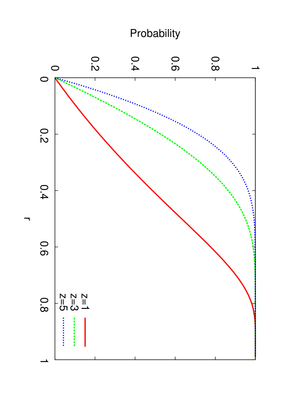
The model is meant to be as general as possible and so the regulatory interactions between genes of successive stages are determined probabilistically, as follows. Each stage $l$ is assigned a regulatory specificity, or simply specificity $s(l)$ with $0\leq s(l)\leq 1$ . A gene $g$ at stage $l$ acts as upstream regulator for a gene $g^{\prime}$ at stage $l+1$ with probability $s^{\prime}(l)=1-s(l)$ . So, the specificity of a developmental stage determines how likely it is for regulatory genes of that stage to cause a state transition of the genes at the next stage; a higher specificity decreases that likelihood.

Our major assumption is that the regulatory specificity increases substantially as development progresses. In other words, the DGEN becomes gradually sparser along the developmental time axis, starting with $s(1)$ $\approx$ 0 and ending with $s(L)$ $\approx$ 1. This assumption is plausible for the following reasons. First, as development progresses the embryo grows in size forming distinct spatial domains. So, extracellular gene regulation becomes more difficult, especially across different domains. Additionally, as development progresses the transitioning genes become more organ- or tissue-specific, implying that their downstream interactions become sparser. Unfortunately, an empirical investigation of the increasing specificity assumption requires knowledge of the complete DGEN for a given species; this is currently not feasible for even the most well-studied model organisms.

The DGEN structural changes we consider are gene deletions, gene duplications, and gene rewiring:

Deletions (DL): This event removes a gene from the DGEN, including its incoming and outgoing edges. There are many genetic mechanisms that may cause such events. A DL event deletes each gene of an individual and at each generation with probability $P_{DL}$ .

Duplication (DP): This event creates an identical copy of a gene $g$ with the same downstream and upstream regulators and at the same developmental stage as $g$ . The two genes may have different fates if one of them is subject later to deletion or rewiring. Otherwise, the two genes are considered identical. A DP event duplicates each gene of an individual and at each generation with probability $P_{DP}$ .

Rewiring (RW): This event changes the upstream and/or downstream regulators of a gene. Changes in the upstream versus downstream regulators may have different biological basis. The former occur, for instance, as a result of mutations in the transcription factor binding sites in a gene’s promoter or mutations in distal regulatory elements such as enhancers, while the latter may be mostly caused by coding sequence mutations. The details of the rewiring process do not affect the results qualitatively as long as the average density of edges in each stage remains consistent with the specificity of that stage. The specific rewiring mechanisms we use are presented next.

Suppose that a RW event affects gene $g$ at stage $l$ . The upstream regulators of $g$ are recomputed based on the specificity of the previous stage, i.e., by choosing each distinct gene of stage $l-1$ with probability $s^{\prime}(l-1)$ . For the downstream regulators of $g$ , we randomly remove $N_{-}$ existing outgoing edges of $g$ , and then add $N_{+}$ outgoing edges to randomly chosen genes of stage $l+1$ that $g$ is not already connected to. Both $N_{-}$ and $N_{+}$ follow a Binomial distribution with $|D(g)|$ trials and success probability $s^{\prime}(l)$ . This captures that the downstream regulators of $g$ are derived by incremental changes in $D(g)$ , instead of giving $g$ a completely new network configuration (thereby, new regulatory function). The higher the regulatory specificity of a stage, the less likely these incremental changes are. An RW event rewires each gene of an individual and at each generation with probability $P_{RW}$ .

A gene deletion or rewiring event at stage $l$ can remove an upstream regulator from genes at stage $l+1$ . A loss of incoming edges may trigger the regulatory failure of a gene, as described next.

Regulatory failures (RF): A gene $g$ may not be able to change functional state if some of its upstream regulators $U(g)$ are lost due to DL or RW events. Even though regulatory networks are often robust to structural perturbations, even a partial gene loss in $U(g)$ may disable $g$ causing a regulatory failure. It is plausible that the probability of a regulatory failure increases with the fraction of lost upstream regulators. So, if $U^{\prime}(g)$ is the new set of upstream regulators and $|U(g)|>|U^{\prime}(g)|>0$ , gene $g$ is removed with probability:

$P_{RF}(r)=1-e^{\frac{-z\,r}{1-r}},\quad 0<r=1-\frac{|U^{\prime}(g)|}{|U(g)|}<1$

while if $|U^{\prime}(g)|=0$ we set $P_{RF}(1)$ =1. $z$ is the RF parameter and it depends on the robustness of regulatory interactions to gene loss.

When a DL or RW event causes one or more RF events, the latter can trigger additional RF events in subsequent developmental stages, leading to cascades of regulatory failures (see Fig.1B). Such RF cascades may cause developmental failure, meaning that the developed embryo is unable to survive or reproduce.

Developmental failure (DF): The last stage of a DGEN represents the fully developed embryo. If that stage includes $\Gamma$ transitioning genes at a successfully developed embryo, the simplest assumption is that an individual with less than $\Gamma$ genes at stage- $L$ has failed to develop properly. Such DGENs are removed from the population and they are replaced with randomly chosen but successfully developed DGENs. We have also experimented with two variations of the DF event: first, the individual is removed if its last stage has less than $\Gamma-\gamma$ genes, where $\gamma$ is small relative to $\Gamma$ , and second, the probability of a DF event increases as the number of genes at stage- $L$ decreases below $\Gamma$ . The qualitative results, as described next, do not change with these two model variations.

Computational Results
We simulate the presented model to examine the properties of the surviving DGENs as evolutionary time progresses. The initial population consists of $N$ identical DGENs with $\Gamma$ genes at each stage. The edges between genes are constructed probabilistically based on the specificity of each stage, as described previously. Simulating the complete model would not show the significance of individual mechanisms such as the increasing specificity assumption. For this reason we construct a sequence of four models with increasing complexity, presenting results separately for each of them:

Model-1: Constant specificity. Each stage has the same specificity, $s(l)$ =0.5 for $l=1\dots L-1$ . Further, this model does not include gene deletion and duplication. Gene rewiring can cause RF and DF events even if there are no DL or DP events.

Model-2: Increasing specificity. The difference from Model-1 is that the specificity is gradually increasing across developmental stages. Unless noted otherwise, the specificity is linear, $s(l)=l/L$ for $l=1\dots(L-1)$ ; a nonlinear specificity function in considered in the SI (see Fig.S12).

Model-3: With gene duplications. Model-3 adds DP events in Model-2. The duplication probability $P_{DP}$ is set so that the average size of a DGEN, across the entire population, stays within a given range (70%-80% of $L\times\Gamma$ genes).

Model-4: With gene deletions. Model-4 adds DL events in Model-3 (complete model). The deletion probability $P_{DL}$ is set so that the average size of a DGEN, across the entire population, stays within the same range as in Model-3.

In Model-1 and Model-2, genes can be only removed (due to RW events, potentially followed by RF cascades) and so the average DGEN size decreases as evolutionary time progresses, which is unrealistic. Model-3 and Model-4 are more realistic because they can maintain a roughly constant DGEN size in the long-term. However, as will be shown next, all aspects of the developmental hourglass effect can already be seen with Model-2 (but not with Model-1). This highlights the increasing specificity assumption as the key property behind the developmental hourglass effect.

Hourglass shape. A first observation is that as evolutionary time progresses, DGENs acquire an “hourglass-like” shape in Models-2,3,4. This means that the width of each stage first decreases until a certain stage (referred to as the waist of the hourglass) and then gradually increases. The hourglass may not be symmetric with respect to the waist. To quantify this observation, we define an “hourglass score” $H$ (see Methods and Fig.S2) that is equal to 1 if the sequence of $L$ stage widths consists of two segments: a decreasing sub-sequence of $k\geq 2$ stages followed by an increasing sub-sequence of $L-k\geq 2$ stages. Fig.2A shows the hourglass score for the population of DGENs in Model-2. Similar graphs for the three other models are shown in the SI (Fig.S3A, Fig.S4A, and Fig.S5A). The $H$ score quickly increases in the three models that have increasing specificity, and it fluctuates close to 1 afterwards.

What is the reason behind the hourglass shape of DGENs? When a gene $g$ is rewired at stage $l$ , it may trigger RF events in stage $l+1$ depending on the number of its lost outgoing edges. In the first few stages, where specificity is low, it is unlikely that a gene would lose a large fraction of its (typically many) incoming edges. In the last few stages, where specificity is high, edges are unlikely to get rewired in the first place. In the mid-stages however, where the specificity is close to 50%, there is higher variability in the number of outgoing edges lost or gained due to RW events. The loss of several outgoing edges due to an RW event at stage $l$ can trigger several RF events and gene removals in the subsequent stage. Thus, the probability of RF events in mid-stages is higher than in early/late stages, making the removal of genes more likely in the former.

The constant specificity of Model-1 does not result in an hourglass pattern (see Fig.S3A) for the following reason. RW events at stage $l$ can cause RF events at the next stage with the same probability, independent of $l$ . However, after the occurrence of an RF event, the size of the potential cascade increases as $l$ decreases simply because there are more subsequent stages to affect. This gives DGENs a “funnel-like” shape with a gradually increasing number of genes after stage-1; $H$ fluctuates around 0.5, as expected for an increasing sequence.

Stage lethality. Another aspect of the developmental hourglass is in terms of the significance of each stage for the survival of the embryo. We define lethality of stage $l$ as the probability that a RW or DL event at stage $l$ starts a RF cascade that eventually leads to a DF event. We estimate this probability at generation $i$ as the fraction of RW and DL events, during the past $i$ generations, that occurred at stage $l$ and led to a DF.

In Model-1, there is no clear trend for the stage lethality probability (see Fig.S3B); with the exception of the last stage (in which RW events cannot result in gene loss), the lethality probability is roughly the same at all stages. In the three models with increasing specificity, however, we observe a clear pattern: the lethality gradually increases until the waist of the hourglass, and then it decreases (see Fig.2B, Fig.S4B, and Fig.S5B). The reason, as explained earlier, is that the probability of RF events in mid-stages is higher that in early/late stages. Additionally, after the formation of the hourglass shape the mid-stages have relatively few genes and so an RF event in those genes is more likely to initiate a lethal RF cascade.

Age of genes. A third aspect of the developmental hourglass effect is related to the evolutionary age of genes. The age of a gene $g$ at generation $i$ is defined as $A(g)=i-t_{0}(g)$ , where $t_{0}(g)$ is the generation at which $g$ was most recently rewired (and 0, if it was not rewired earlier). The rationale behind this definition is that a rewiring event may give that gene a new function, at least in terms of its upstream and downstream regulators.

In the case of Model-2, Fig.2C shows the median age of the genes at each stage, considering the population of all genes across all individuals at a given generation. See Fig.S3C, Fig.S4C, and Fig.S4C for the same results with the three other models. The evolutionary age at stage $l$ follows the same pattern as the lethality probability: it gradually increases until we reach the waist of the hourglass, and then it gradually decreases. Genes at intermediate stages tend to be older because, as explained earlier, they are fewer and their rewiring is more likely to be lethal. When one of those genes $g$ is rewired or deleted from a DGEN, the corresponding individual is often replaced (DF event) by another individual that has the same gene $g$ . So, the genes at the waist of a DGEN tend to be more conserved than genes at earlier or later stages.

Data Analysis
We have examined the predictions of the previous model using transcriptome data for Drosophila melanogaster and Arabidopsis thaliana. We summarize the Drosophila results here; the corresponding figures for A.thaliana can be found in the SI (Fig.S9 and Fig.S10). For Drosophila, we analyze Microarray [11] and RNA-Seq [25] temporal expression profiles during the first 20 hours of development, taken at 10 stages of 2-hr intervals. We examine whether a) the number of transitioning genes follows an hourglass pattern, b) the waist of that hourglass coincides with the Drosophila phylotypic stage, and c) the evolutionary age of the transitioning genes follows a similar hourglass pattern. The two datasets are described in more detail in the Methods section. With such limited data, we cannot infer the regulatory edges between transitioning genes and we cannot reconstruct the underlying DGEN. However, we can identify the transitioning genes at each developmental stage given a “transition threshold” $c$ (see Methods). Even though the correct value of this threshold is not known the following results are robust in a wide interval of $c$ , which includes most of the expression variation range across successive developmental stages (see Fig.S8 for the CDFs of expression level variations across successive stages).

Fig.3A and Fig.3B show the hourglass resemblance score H (and its more robust variant) as function of $c$ . Note that the H score is close to 1 for a wide range of $c$ , confirming the presence of an hourglass-like structure in terms of the number of transitioning genes. Fig.3G and Fig.3H exhibit this pattern more clearly in the number of transitioning genes for a specific value of $c$ . The two datasets also show reasonable agreement in terms of the assignment of transitioning genes to stage-pairs (see Fig.S6).

Second, the location of the waist in this hourglass pattern, shown in Fig.3C and Fig.3D, occurs at the stage-pair (3,4) or (4,5), depending on $c$ . This is roughly 8 hours after the formation of the zygote, and it includes the phylotypic stage for Drosophila melanogaster [11].

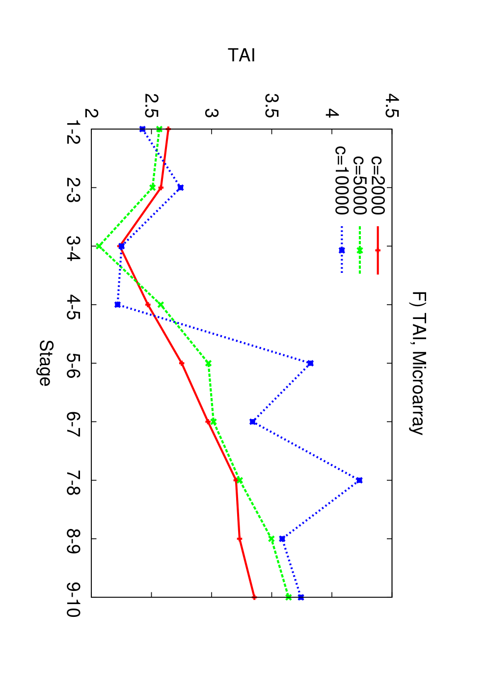
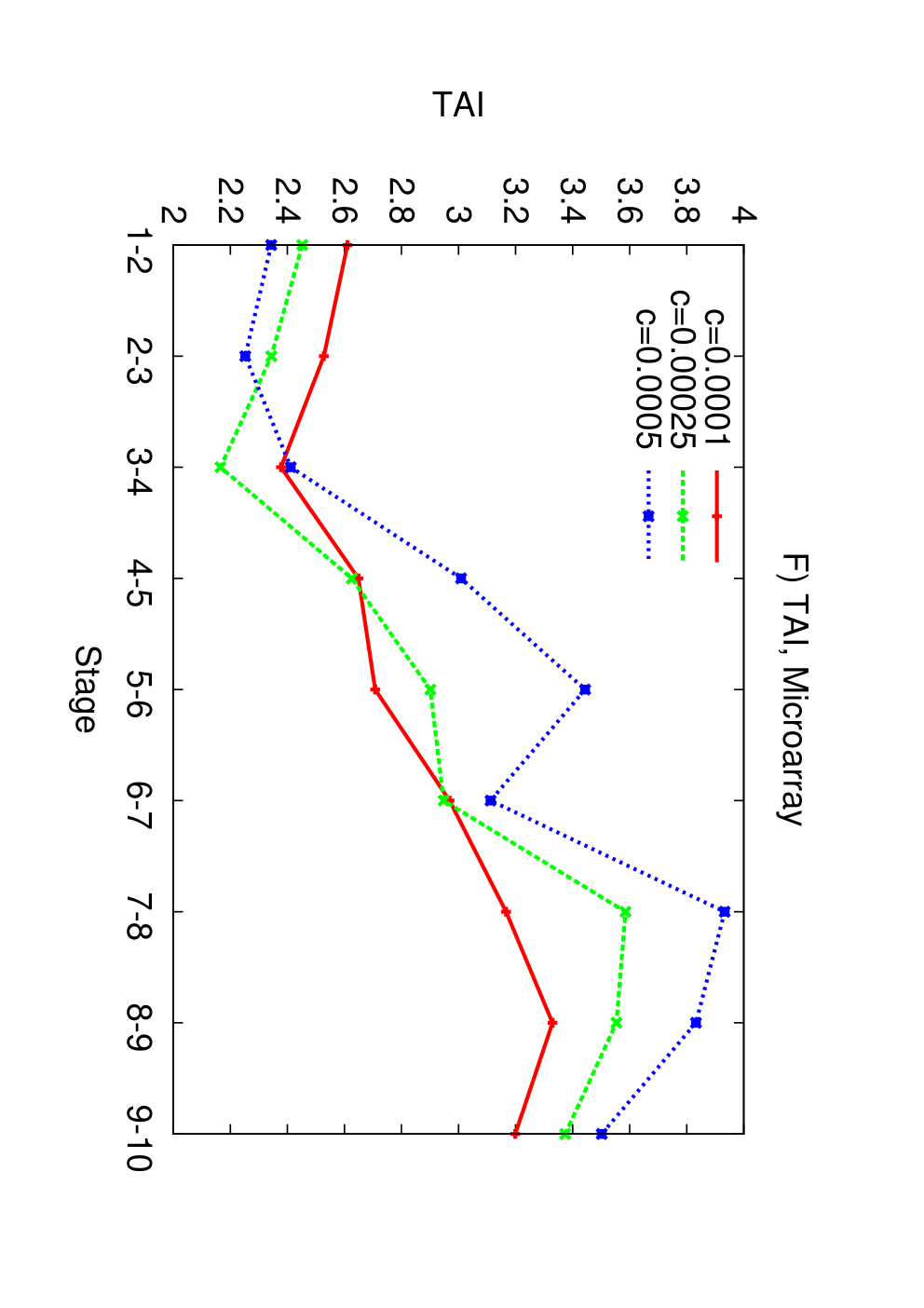
We have also estimated the evolutionary age of most of the transitioning genes at each developmental stage-pair using the Transcriptome Age Index (TAI) metric [14] (see Methods). TAI is lower for older genes. Fig.3E and Fig.3F show the average TAI for transitioning genes, weighted by the expression level of each gene, at each stage-pair and for each dataset using three values of $c$ . The TAI index follows the pattern that the model predicts, with older genes (lower TAI values) close to the waist of the hourglass. This result appears consistent with the main observation of Domazet-Loso and Tautz [14], even though that study did not analyze transitioning genes.

Discussion
Early studies of the developmental hourglass effect mostly analyzed morphological and phenotypic similarities across species [26, 3]. Recently, the focus has shifted towards genomic and molecular comparative studies [14, 10, 11, 21, 13] that investigate conservation of gene expression variation, sequence conservation, selective constraint on coding sequences, and evolutionary gene “age.” These studies often report contradicting observations: some support strong conservation in earlier developmental stages [7, 8, 21], while others support that strongest conservation occurs at a mid-developmental stage [9, 10, 11, 12, 13, 15, 14, 16, 17]. Nevertheless, the fact that the hourglass effect is observed in highly divergent species across deep phylogenetic scales (including fish, flies and plants), suggests that this observed pattern of conservation may stem from fundamental organization principles.

What these principles are has remained elusive. Earlier stages may be conserved because any changes therein could have large cascading effects in later stages [27, 28, 7]. Later stages may experience less constraint because as development progresses gene interactions become more modular, and so it is plausible that perturbations there have only local effects [2]. We refer to them as the “temporal” constraint model and the “spatial” constraint model, respectively, following Tian et al. [29].

In this paper, we developed an evolutionary model of development that combines some aspects of the previous two models. Regulatory perturbations at a certain stage can cause cascades of regulatory failures at subsequent stages (temporal model), while the likelihood that a gene regulates genes at a subsequent stage decreases as development progresses (spatial model). Our computational results lead to the following testable predictions: a) the number of transitioning genes during development follows an hourglass pattern, b) the evolutionary age of the transitioning genes also follows an hourglass pattern, with the oldest genes being at the waist of the hourglass, and c) the genes at the waist of that hourglass are the most essential, in the sense that their deletion maximizes the probability of developmental failure. We have relied on developmental gene expression profiles of Drosophila melanogaster and Arabidopsis thaliana to examine the predictions of the model. The analysis of that data agrees with the first two theoretical model predictions. The increased conservation of genes at the waist provides an indirect confirmation of the model’s third prediction, regarding the essentiality of different genes. Further, our simulations confirm that the details of these regulatory perturbations, such as the probabilities of gene duplication and deletion or the parameter $z$ in the regulatory failure probability, do not affect the results of the model, at least at the qualitative level.

The use of DGENs in this work was only as an abstract tool to study the effect of gene regulatory perturbations in the developmental process. In future work, it is important to infer the actual DGEN of model organisms. This will require information about gene regulatory interactions across time and space, but it should be possible for at least some developmentally well studied species [24]. Such DGENs would help to identify the specific genes that form the hourglass waist and their function. Additionally, an inferred DGEN would allow to directly test the increasing specificity assumption.

Finally, we note that the hourglass effect (sometimes referred to as the “bow tie” effect) has also been observed in other complex biological and technological systems that exhibit hierarchical modularity and that are subject to evolutionary pressure or optimization trade-offs [30, 31, 32, 33]. For instance, the Internet “protocol stack” is organized in an hourglass structure [35]; this pattern was not designed but it emerged through the competition between protocols that serve roughly the same function at each communication layer, during the last 30-40 years. In earlier work, we proposed an abstract model (EvoArch) that captures the evolution of protocol architectures and that predicts the emergence of an hourglass structure. Interestingly, both EvoArch and the model of this paper share the same principle: the underlying hierarchical networks that control both systems should be increasingly sparser as complexity increases, i.e., the specificity of each complexity stage (or layer) should be increasing. In the future, we will further investigate this common organization principle between biological and technological systems.

Materials and Methods
Hourglass score H. Suppose that $w(l)$ denotes the number of transitioning genes in stage $l$ and let $b$ be the stage with the minimum number of such genes. We construct the sequences $X$ = $\{w(l)\},l=1,\dots b\}$ and $Y$ = $\{w(l)\},l=b,\dots L\}$ . $\tau_{X}$ and $\tau_{Y}$ denote the normalized univariate Mann-Kendall statistic for monotonic trend in each sequence, respectively ( $\tau$ is -1 for decreasing, +1 for increasing and almost 0 for random sequences). The H score is defined as $H=(\tau_{Y}-\tau_{X})/2$ . See Fig.S2 for an illustration, and for the definition of a more robust version of H.

Drosophila data and treatment. Developmental gene expression profiles are obtained from two sources. First, microarray data from Kalinka et al. [11] for 3,610 genes. The expression level of each gene is calculated as the median of probes mapping to that gene. Each stage represents a 2-hr interval during the first 20 hours of embryogenesis (10 stages). The second source is RNA-Seq data from Graveley et al. [25]. Raw data are processed to RPKM values. Each stage represents a 2-hr interval during the first 24 hours (12 stages). Genes with zero RPKM value in all stages are discarded, resulting in 14,110 genes.

Transitioning gene identification. Suppose that the reported expression value of gene $i$ at stage $l$ is $e_{i,l}$ . We analyze both these “absolute” expression values as well as the normalized expression values, given by $e^{\prime}_{i,l}$ = $e_{i,l}/\sum_{j}e_{j,l}$ . The identification of transitioning genes follows the same method for both absolute and normalized expression levels. In the case of normalized expressions, we calculate $\delta_{i,l}=e^{\prime}_{i,l}-e^{\prime}_{i,l-1}$ for each gene and at each stage $l$ = $2\dots L$ . Gene $i$ is considered “transitioning” at the stage-pair $(l-1,l)$ if $|\delta_{i,l}|>c$ , where $c$ is a given transition threshold. This condition is more robust to noise than a ratio-based rule ( $e^{\prime}_{i,l}/e^{\prime}_{i,l-1}$ ) for the identification of transitioning genes. Note that a gene may be transitioning at more than one stage-pair, but it may also not be transitioning at any stage-pair.

Transcriptome age index (TAI). We collected the groups of orthologs for each gene in Drosophila using two databases, OrthoDB [37] and OrthoMCL [38]. The Eumetazoa data were taken from OrthoDB, while Fungi and Plants species were retrieved from OrthoMCL, and the two datasets were merged. Using these orthologs we then assigned an age index to each gene based on its absence and presence in a phylogenetic tree of 24 well-diverged species [14, 13] (see Fig.S14).

Age index for each stage-pair. Suppose that we identify transitioning genes based on the normalized expression levels, and that $n(l)$ genes are assigned to stage-pair $(l-1,l)$ . Denote by $p_{i}$ the phylogenetic rank (TAI value) of gene $i$ . The age index assigned to that stage-pair is given by TAI(l)= $(\Sigma_{i=1}^{n(l)}p_{i}e^{\prime}_{i,l})/\Sigma_{i=1}^{n(l)}e^{\prime}_{i,l}$ . The same method is used when transitioning genes are identified based on absolute expression levels.

References

[1] Carroll SB (2005) Endless Forms Most Beautifull: The New Science of Evo Devo and the Making of the Animal Kingdom (WW Norton & Company) No. 54.
[2] Raff RA (1996) The shape of life: genes, development, and the evolution of animal form.
[3] Richardson MK, Keuck G (2002) Haeckel’s abc of evolution and development. Biological Reviews 77:495–528.
[4] Davidson EH (2010) The regulatory genome: gene regulatory networks in development and evolution (Academic Press), 2nd edition.
[5] Duboule D (1994) Temporal colinearity and the phylotypic progression: a basis for the stability of a vertebrate bauplan and the evolution of morphologies through heterochrony. Development 1994:135–142.
[6] von Baer CE (1828) Über Entwicklungsgeschichte der Thiere. Beobachtung und Reflexion.-Königsberg, Gebrüder Bornträger 1828-1837 (Gebrüder Bornträger) Vol. 1.
[7] Rasmussen N (1987) A new model of developmental constraints as applied to the drosophila system. J Theor Biol 127:271–299.
[8] Roux J, Robinson-Rechavi M (2008) Developmental constraints on vertebrate genome evolution. PLoS Genet 4:e1000311.
[9] Irie N, Kuratani S (2011) Comparative transcriptome analysis reveals vertebrate phylotypic period during organogenesis. Nat Commun 2:248.
[10] Irie N, Sehara-Fujisawa A (2007) The vertebrate phylotypic stage and an early bilaterian-related stage in mouse embryogenesis defined by genomic information. BMC Biol 5:1.
[11] Kalinka AT, et al. (2010) Gene expression divergence recapitulates the developmental hourglass model. Nature 468:811–814.
[12] Levin M, Hashimshony T, Wagner F, Yanai I (2012) Developmental milestones punctuate gene expression in the caenorhabditis embryo. Dev Cell 22:1101–1108.
[13] Quint M, et al. (2012) A transcriptomic hourglass in plant embryogenesis. Nature 490:98–101.
[14] Domazet-Lošo T, Tautz D (2010) A phylogenetically based transcriptome age index mirrors ontogenetic divergence patterns. Nature 468:815–818.
[15] Hazkani-Covo E, Wool D, Graur D (2005) In search of the vertebrate phylotypic stage: a molecular examination of the developmental hourglass model and von baer’s third law. J Exp Zool B Mol Dev Evol 304:150–158.
[16] Galis F, Metz JA (2001) Testing the vulnerability of the phylotypic stage: on modularity and evolutionary conservation. J Exp Zool 291:195–204.
[17] Cruickshank T, Wade MJ (2008) Microevolutionary support for a developmental hourglass: gene expression patterns shape sequence variation and divergence in drosophila. Evol Dev 10:583–590.
[18] Comte A, Roux J, Robinson-Rechavi M (2010) Molecular signaling in zebrafish development and the vertebrate phylotypic period. Evol Dev 12:144–156.
[19] Hall BK (1997) Phylotypic stage or phantom: is there a highly conserved embryonic stage in vertebrates? Trends Ecol Evol 12:461–463.
[20] Kalinka AT, Tomancak P (2012) The evolution of early animal embryos: conservation or divergence? Trends Ecol Evol 27:385–393.
[21] Piasecka B, Lichocki P, Moretti S, Bergmann S, Robinson-Rechavi M (2013) The hourglass and the early conservation models—co-existing patterns of developmental constraints in vertebrates. PLoS Genet 9:e1003476.
[22] Richardson MK, Minelli A, Coates M, Hanken J (1998) Phylotypic stage theory. Trends Ecol Evol 13:158.
[23] RP BEO, Richardson MK, et al. (2003) Inverting the hourglass: quantitative evidence against the phylotypic stage in vertebrate development. Proc R Soc Lond B Biol Sci 270:341–346.
[24] Peter IS, Faure E, Davidson EH (2012) Predictive computation of genomic logic processing functions in embryonic development. Proc Natl Acad Sci USA 109:16434–16442.
[25] Graveley BR, et al. (2010) The developmental transcriptome of drosophila melanogaster. Nature 471:473–479.
[26] Richardson MK, et al. (1997) There is no highly conserved embryonic stage in the vertebrates: implications for current theories of evolution and development. Anat Embryol (Berl) 196:91–106.
[27] Riedl R, Jefferies RPS (1978) Order in living organisms: a systems analysis of evolution (Wiley New York).
[28] Arthur W (1984) Mechanisms of morphological evolution: a combined genetic, developmental, and ecological approach (Wiley New York).
[29] Tian X, Strassmann JE, Queller DC (2013) Dictyostelium development shows a novel pattern of evolutionary conservation. Mol Biol Evol 30:977–984.
[30] Beutler B (2004) Inferences, questions and possibilities in toll-like receptor signalling. Nature 430:257–263.
[31] Csete M, Doyle J (2004) Bow ties, metabolism and disease. Trends Biotechnol 22:446–450.
[32] Doyle JC, Csete M (2011) Architecture, constraints, and behavior. Proc Natl Acad Sci USA 108:15624–15630.
[33] Tieri P, et al. (2010) Network, degeneracy and bow tie integrating paradigms and architectures to grasp the complexity of the immune system. Theor Biol Med Model 7:32.
[34] Zhao J, Yu H, Luo JH, Cao ZW, Li YX (2006) Hierarchical modularity of nested bow-ties in metabolic networks. BMC Bioinformatics 7:386.
[35] Akhshabi S, Dovrolis C (2011) The Evolution of Layered Protocol Stacks Leads to an Hourglass-Shaped Architecture.
[36] Akhshabi S, Dovrolis C (2013) in Dynamics On and Of Complex Networks, Volume 2 (Springer), pp 55–88.
[37] Waterhouse RM, Tegenfeldt F, Li J, Zdobnov EM, Kriventseva EV (2013) Orthodb: a hierarchical catalog of animal, fungal and bacterial orthologs. Nucleic Acids Res 41:D358–D365.
[38] Li L, Stoeckert CJ, Roos DS (2003) Orthomcl: identification of ortholog groups for eukaryotic genomes. Genome Res 13:2178–2189.
[39] Xiang D, et al. (2011) Genome-wide analysis reveals gene expression and metabolic network dynamics during embryo development in arabidopsis. Plant Physiol 156:346–356.