Cosmology with Minkowski functionals and moments of the weak lensing convergence field
Abstract
We compare the efficiency of moments and Minkowski functionals (MFs) in constraining the subset of cosmological parameters using simulated weak lensing convergence maps. We study an analytic perturbative expansion of the MFs ([1, 2]) in terms of the moments of the convergence field and of its spatial derivatives. We show that this perturbation series breaks down on smoothing scales below , while it shows a good degree of convergence on larger scales (). Most of the cosmological distinguishing power is lost when the maps are smoothed on these larger scales. We also show that, on scales comparable to , where the perturbation series does not converge, cosmological constraints obtained from the MFs are approximately 1.5-2 times better than the ones obtained from the first few moments of the convergence distribution — provided that the latter include spatial information, either from moments of gradients, or by combining multiple smoothing scales. Including either a set of these moments or the MFs can significantly tighten constraints on cosmological parameters, compared to the conventional method of using the power spectrum alone.
Keywords:
Weak gravitational lensing — Data analysis — Methods: analytical, numerical, statisticalI Introduction
Weak gravitational lensing (WL) surveys will be able to probe cosmology with unprecedented accuracy, tightening present constraints on some cosmological parameters by over an order of magnitude. With recent results from the first large WL surveys (COSMOS: [3, 4] and CFHTLenS: [5, 6]), the question of how to extract the maximum amount of information from weak lensing shear and convergence maps is becoming more pressing. The power spectrum, or equivalent two point statistics, are of unquestionable importance in this investigation, but are inevitably incomplete if non-Gaussian features are present. This is precisely the case when one studies weak lensing, because gravity is non linear and generates non-Gaussian features on small scales. The most straightforward way to characterize non-Gaussian fields is by using higher order polyspectra, correlation functions or moments [7, 8, 9, 10, 11]. An interesting and less explored alternative, originally proposed in the context of the 3D cosmological matter density field, is to use topological descriptors [12]; one kind of such descriptors are the Minkowski functionals [13]. [14] studied the effects of primordial non-Gaussianity on the topology of large-scale structures, measuring three-dimensional MFs on simulated density fields. [15] used a next-to-leading order perturbative expansion of the MFs to derive constraints on the matter density parameters using a limited number of simulated weak lensing shear maps. A second early paper on MFs applied to weak lensing was written by [16], which used these descriptors to discern between the SCDM, OCDM and CDM cosmological models. [2] have studied a perturbation series for the MFs in harmonic space to isolate the contribution of different modes to each MF. Using ray-tracing N-body simulations, [17] have recently shown that the MFs of the convergence field can tighten constraints on dark energy parameters by a factor of 3 compared to using the power spectrum alone. In this work we analyze and compare the effectiveness of the MFs and multi-point moments of the convergence field in extracting cosmological information. Throughout this paper, we use the term multi-point moments to mean moments of the convergence field itself, as well as of its spatial derivatives. There exists a perturbative expansion of the MFs in terms of the multi-point moments ([1, 2]). In this work, we investigate whether this expansion converges, both in the conventional sense of accurately reproducing the MFs, and also in the sense of capturing the cosmological information contained in the MFs. The rest of this paper is organized as follows. In § II we give an overview of the known properties of MFs in § III we explain the methods we used to analyze our set of simulated maps, the results of which are summarized in § IV. The results we obtained, along with a discussion, are presented in § IV and § V. Finally, in § VI we present our conclusions, along with a few caveats and possible follow-ups to this project.
II Formalism
II.1 Minkowski functionals
MFs are topological descriptors of two-dimensional random fields that have proven very useful in describing their statistical properties. Given a two-dimensional random field (in our case the convergence field) of zero mean and variance , we can consider its excursion sets that consist of all the points at which the field exceeds a particular threshold value (see Figure 1 for an illustrative example).
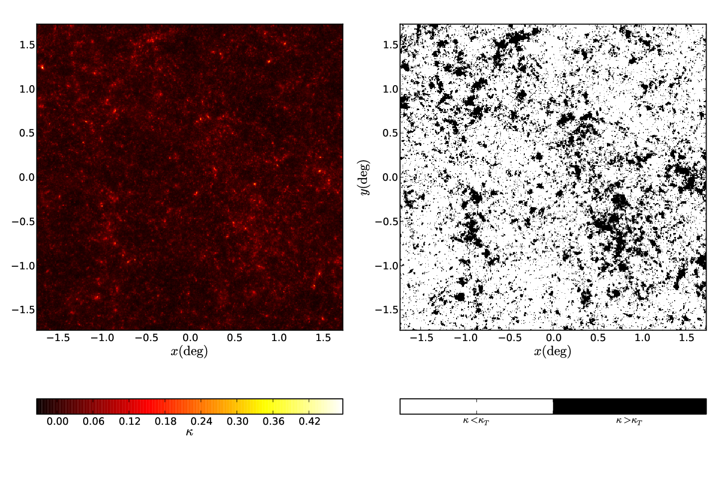
The three MFs and measure respectively the area, length of the boundary and genus characteristic of these excursion sets
| (1) |
| (2) |
| (3) |
where is the total area of the map, and are the area and boundary length elements, respectively, and is the curvature of the boundary. Following the notations of [14] and [2], in the above equations denotes the excursion set boundary. is a measurement of the cumulative one point PDF of the convergence field, while and contain spatial information on the excursion sets and are sensitive to -point correlation properties for arbitrary high . is related to the genus of the excursion set and is equal to the number of connected regions above the threshold (“islands”), minus the number of connected regions below the threshold (“holes”). For high thresholds is nearly equal to the number of convergence peaks [18]. If the underlying random field is perfectly Gaussian, there is a one-to-one correspondence between the power spectrum of the field and the [19, 20]. For non-Gaussian fields, however, it is known that the MFs are sensitive to all the multi-point correlations functions, which can be used to construct a perturbative approximation [1].
II.2 Perturbation series
An exhaustive analytic study of the perturbative expansion of the MFs has recently been presented by [2]. These authors have modeled in detail the harmonic-space structure of the convergence power spectrum and bispectrum, using the halo model. In the present work, we do not consider such a fine level of detail, because we are interested only in those components of the power spectrum and the bispectrum that enter the actual perturbation expansion. In order to build a perturbative approximation to the MFs, we follow [1] and note that equations (1)-(3) can be conveniently expressed in terms of spatial average values of derivatives of the convergence field. Approximating the maps as flat, we introduce two coordinates and use the notations , and , with which one can write
| (4) |
| (5) |
and
| (6) |
where is the step function and is the Dirac delta function. The factor in equation (5) comes from the fact that for isotropic fields , and an analogous relation can explain the factor of in equation (6). It can be shown that these averages can be expressed in a convenient form using the variance of the convergence field, , and the variance of its gradient, , as follows
| (7) |
Here is the measure of the solid angle in dimensions and hence and . In the Gaussian case (see [19, 20]), the normalized MFs take the very simple form
| (8) |
where is the -th Hermite polynomial,
| (9) |
When non–Gaussianity is present, the functions can be expanded in a Taylor series in powers of , whose coefficients depend on the higher-order moments of the random field. These higher moments characterize the non–Gaussianity. In particular, we can write
| (10) |
The series coefficients will, in general, contain the information on the higher–order moments of the distribution, such as the skewness and the kurtosis. These coefficients take the general form
| (11) |
As an example, the first term () in the expansion (eq. 10) is given by [1]
| (12) |
where
| (13) |
Note that this term is determined entirely by the three skewness parameters (13). The next to leading order corrections () are similarly given by a weighted sum of the four connected kurtosis parameters.
| (14) |
In this work by ”connected” we mean the non-Gaussian components of the moments: for Gaussian fields we have that , so that the connected part is a measure of the second order non-Gaussianity. In the Gaussian case the skewness parameters are zero, and hence they coincide with their connected part. The expressions for these next-to-leading-order corrections are lengthy and do not add anything to the present discussion; we refer the interested reader to [1] for the complete set of equations. However, it is worth pointing out a relevant property of the expansion series. Since does not contain any spatial or morphological information about the field, it makes sense that its perturbation series, at all orders, will be entirely determined in terms of the one point cumulants . In contrast, the moments with derivatives, which contain spatial information, will appear in the expansion of both of the other two MFs. In order to have any hope that the series convergences, it must be that the higher order cumulants become smaller and smaller as grows, i.e. it is necessary that as grows. When the departure from a Gaussian field is significant, this is generally not the case — the series then does not converge, and the MFs do not admit a perturbative expansion. In the case of temperature maps of the cosmic microwave background (CMB), which are almost Gaussian, it has been shown (e.g. [1, 21]) that the series converges accurately, also because the simple Gaussian approximation is good enough. Given the much larger non-Gaussianities in the WL convergence field, it is not guaranteed that the series will converge when applied to WL. A goal of the present study is to quantify how well (or not) the WL series converges.
III Methods
III.1 N-body simulations and ray-tracing
In order to understand if the weak lensing MFs admit a perturbative expansion in terms of multi-point moments, we must evaluate the series numerically and compare it to the actual MFs measured from simulated maps. For this purpose, we use a large suite of simulated convergence maps (see [17]), generated with a two-dimensional ray-tracing algorithm (see [22]), for a number of different combinations of the three cosmological parameters , referring respectively to the matter density, the equation of state of dark energy and the normalized amplitude of the initial density fluctuations, as summarized in Table 1.
| Description | Number of simulations | |||
|---|---|---|---|---|
| Fiducial | 0.26 | -1.0 | 0.798 | 45 |
| Auxiliary | 0.26 | -1.0 | 0.798 | 5 |
| Low | 0.23 | -1.0 | 0.798 | 5 |
| High | 0.29 | -1.0 | 0.798 | 5 |
| Low | 0.26 | -1.2 | 0.798 | 5 |
| High | 0.26 | -0.8 | 0.798 | 5 |
| Low | 0.26 | -1.0 | 0.750 | 5 |
| High | 0.26 | -1.0 | 0.850 | 5 |
For each choice of cosmological parameters we have (pseudo-)independent realizations of the convergence field for each of three fixed source galaxy redshifts and 2. Each realization is a flat 12 deg2 map with a pixel resolution of and pixels per side. We call these realizations (pseudo-)independent because they are drawn from the same set of simulations, rotating the lens planes from which the ray tracing is performed. We add galaxy shape noise, , to each of the realizations, following a conventional approach (see for example [17]) to model this noise as a white Gaussian noise with real space correlation function
| (15) |
Here is the number density of source galaxies, which we assume to be , is the Kronecker delta tensor and each pixel is specified by its two coordinates . We assume that this noise has an amplitude equal to that of one component of the shear, and so has an r.m.s. value (see [23])
| (16) |
After adding the noise, we smooth each map with a Gaussian window function of angular size and kernel
| (17) |
Throughout this paper, we refer to the parameter as the smoothing scale of our maps; for reference, the maps are stored in FITS format and the input is processed with the CFITSIO library [24]; the smoothing is performed in Fourier space for computational time speedup using the FFTW3 C library [25].
III.2 Observables from simulated lensing maps
For each map, we measure a set of multi–point moments and MFs with linear size threshold bins. We limit our perturbation series expansion to order and, motivated by equations (13), (14), we measure the nine moments for each realization ; gradients are calculated with first order finite difference looking at the values of the nearest neighboring pixels, assuming periodic boundary conditions. For the direct measurement of the MFs we again follow [17] and express the spatial averages (4),(5) and (6) as integrals over the map planes
| (18) |
| (19) |
| (20) |
In equations (18)-(20) the integrals are calculated as discrete sums over pixels and the derivatives are evaluated via finite difference with periodic boundary conditions. For large smoothing scales , the denominator in the integrand of expression (20) can vanish on some of the pixels; this is an issue especially for large smoothing scales, when neighboring pixels can acquire similar values, making gradients vanish. To deal with this, when this happens, we take the explicit limit with and replace the integrand with the expression . The direction in which to take this limit is arbitrary, but the difference between one choice and the other is of relative order and hence can be safely neglected. To approximate the functions we use discrete binning for the thresholds and we divide the interval in parts of equal size. This discretization choice leads to rounding errors for the MFs, which have been investigated by [17]. We then save these binned MFs in a vector of size , for each realization . Our complete set of descriptors is then a dimensional vector . We measure this entire set of descriptors for each of the 1000 realizations for each cosmological model, using 100 cores at the BNL Astro Cluster. Parallelization is implemented with the MPI library [26].
III.3 Forecasting cosmology constraints
To measure the information content (i.e. the constraining power) that each of our descriptors carries, we want to calculate the error on each of the cosmological parameters that results from using a particular set of descriptors. To begin, we measure the averages and the covariance matrix of our descriptors using the 1000 realizations available,
| (21) |
and
| (22) |
Before using this information to fit for the cosmological parameters, we can ask ourselves how well our set of descriptors is able to discriminate between two different cosmological models. We have quantified this difference using a analysis, and we computed the quantity
| (23) |
Note that repeated indices and are summed over, and that the superscripts and in equations (22) and (23) have different meanings: in the former case we refer to the superscript as the particular realization we are analyzing, in the latter as the particular cosmological model considered. The quantity measures how well a set of descriptors is able to discriminate between two different cosmological models, typically the fiducial v.s. one of the alternative models in Table 1. We use the same set of descriptors to find the best-fit cosmological parameters [with ] for each realization; this allows us to compute the parameter covariance matrix . We use a linear interpolation between the fiducial and the alternative cosmologies to model the dependence of each descriptor on the cosmological parameters,
| (24) |
with is evaluated as a forward finite difference derivative. In each realization (of the fiducial cosmology), we find the best-fit cosmological parameters by minimizing the ,
| (25) |
with respect to (note that is a vector of the three cosmological parameters). We want to stress the difference in meaning by the two statistics (23),(25): the former is a measure of the cosmological distinguishing power of a particular set of descriptors, the latter is a function of , which minimum represents the best fit parameter values for an individual realization. With the linear interpolation (24), this minimization can be done by solving analytically. This minimization condition translates to
| (26) |
The solution to this linear system is given in terms of the differences and inverse matrices,
| (27) |
We can also calculate the parameter covariance matrix analytically, in terms of the covariance matrix of the descriptors, using equation (27) and the fact that ; matrix manipulations give us
| (28) |
The final result of this calculation is the inverse of the familiar Fisher matrix , except neglecting the dependence of the (co)variances on cosmology ([27, 28]); we should stress that this statement holds only because we chose to perform the fitting of the cosmological parameters linearly interpolating our observables set between different cosmological models. We should also note that the marginalized errors calculated from this analytical covariance matrix correspond to “one sigma”, or confidence level only if the fluctuations of the observables between realizations are Gaussian. We have no reasons apriori that this would be the case for the weak lensing MFs and moments. On the other hand, the above approach directly yields the full likelihood analytically (since we have the best-fit parameters for each realization), and allows us to go beyond the Fisher matrix and relax this Gaussian assumption. Further details and discussion of this point will be included in § IV.3 below. There is an additional complication: as we will clarify in § V.4, we have reasons to think that this picture is oversimplified and that the parameter error bars that one gets from equation (28) are underestimated when the descriptor set (and in particular the number of thresholds for the MF, ) is too large. To correct this underestimation, we take advantage of the fact that we have at our disposal two different set of maps for the fiducial cosmology, generated respectively from 5 and 45 simulations. We use one set of maps, , to measure the covariance matrix which we use to construct the in equation (25); we call this covariance matrix . We use the other set of maps, , to fit the cosmological parameters; that is to say in equation (25) the observables are measured from the set of maps so that is the covariance matrix measured from set . This leads to a more complicated expression for the parameter covariance, which can be generalized as
| (29) |
with the convenient notation . As pointed out by [17], the covariance matrices measured from different set of maps (obtained with 5 and 45 simulations) are not the same and equation (29) can lead to quite different (but more accurate) results than the simpler equation (28). In the present discussion, we didn’t mention the fact that equations (23) and (28) need to be corrected by a multiplying factor of due to the fact that the estimator that we use for the inverse of the covariance matrix, , is biased (see [29, 30]); for our set of MFs binned with this accounts for a 10% correction, which is small enough not to affect any of our conclusions below. The finding that equation (28) underestimates error bars is not due to the fact that it misses the correction factor, but to the fact that the correlation between the observables vector and the covariance matrix forces us to use different set of maps, and in particular equation (29) to obtain the correct sized error bars. Throughout the discussions below, the errors are calculated as where and refer to the sets of fiducial maps obtained respectively from 5 and 45 simulations; the errors are scaled by the constant factor , where is the approximate ratio of the solid angle covered by the LSST survey (20,000 deg2; [31]) to the area of one of our simulated maps (12 deg2).
IV Results
IV.1 Numerical MF measurement accuracy
To check the accuracy of our code, we have created 1,000 realizations of a Gaussian random field, with the same size as our weak lensing maps (see [17]) and measured the three MFs with the procedure in § III.2. We have used , choice that will be justified in § V.4
The results are shown, together with the analytic expectations from equations (7) and (8), in Figure 2.

As this figure shows, our code measures the MFs for a Gaussian random field highly accurately, with relative residuals smaller than one part in . Although [17] achieved somewhat better accuracy, the accuracies in Figure 2 are sufficient for our purposes, and will not influence our conclusions on the convergence of the perturbation series. We will discuss this point further in § V below.
IV.2 Perturbation series convergence
We next test the convergence of the perturbation series in equation (10) up to order , i.e. up to the contributions containing the fourth order cumulants. We compared the residuals with the differences in that we obtain when varying the cosmological parameters ; we again used . The MFs from the analytical series expansion, , are calculated by measuring the moments for each of the 1000 realizations, taking the average, and then using equations (7) to (14). The results are displayed in Figures 3 and 4, for both the noisy and the noiseless maps, and for different smoothing scales. One expects that for a sufficiently large smoothing scale, the field becomes close to Gaussian, and the perturbation series is convergent. We investigated this issue in Figure 5, where we show the difference (calculated with equation (23)) between the measured and perturbative expanded MFs as a function of the perturbative order and smoothing scale used. If the series is convergent, an important question to ask is if the MFs are still effective in distinguishing different cosmological models. To answer this question, we computed the values as in equation (23) for each of the smoothing scales we tested, and for three deviations from the fiducial cosmology, summarizing the results in Table 2. We used the same statistic to quantify the convergence of the perturbation series, and see how this compares to the difference in cosmological models.


| (arcmin) | ||
|---|---|---|
| Noiseless | Noisy | |
| Analytical - measurement comparison () | ||
| 1 | ||
| 5 | 7.65 | 5.79 |
| 15 | 0.45 | 0.34 |
| High | ||
| 1 | 32.45 | 9.32 |
| 5 | 5.48 | 3.86 |
| 15 | 1.47 | 1.18 |
| High | ||
| 1 | 20.60 | 2.67 |
| 5 | 2.37 | 1.59 |
| 15 | 1.47 | 1.13 |
| High | ||
| 1 | 21.06 | 12.84 |
| 5 | 6.42 | 5.14 |
| 15 | 1.47 | 1.44 |
IV.3 Information content and constraining power
We calculated the marginalized errors in the cosmological parameters analytically using equation (29) for various sets of descriptors, in order to distinguish the constraining power of the MFs and the moments. We chose again to obtain realistic constraints: as already stressed this choice will be justified later in § V.4. The results are summarized in Table 3 and will be discussed in § V below
| Descriptors | |||
|---|---|---|---|
| One point moments | |||
| Unconnected () | 0.0066 | 0.035 | 0.0069 |
| Connected () | 0.0051 | 0.025 | 0.0053 |
| All moments (connected) | |||
| Add | 0.0017 | 0.0089 | 0.0023 |
| Add | 0.0016 | 0.0088 | 0.0022 |
| Add | 0.0016 | 0.0082 | 0.0021 |
| Add | 0.0016 | 0.0082 | 0.0021 |
| Add | 0.0016 | 0.0082 | 0.0021 |
| Add | 0.0015 | 0.0081 | 0.0020 |
| Smoothing scale combination | |||
| 0.0020 | 0.012 | 0.0025 | |
| 0.0016 | 0.0092 | 0.0021 | |
| 0.0019 | 0.010 | 0.0024 | |
| 0.0017 | 0.0090 | 0.0022 | |
| Minkowski functionals | |||
| 0.0015 | 0.0073 | 0.0019 | |
| 0.0013 | 0.0065 | 0.0018 | |
| 0.0014 | 0.0067 | 0.0020 | |
| 0.00096 | 0.0052 | 0.0014 | |
| Minkowski functionals + All moments | |||
| 0.00096 | 0.0051 | 0.0014 | |
We have investigated the errors in Table 3 and checked if these numbers do correspond to a 68.4%, or one , confidence level. Significant differences can arise if the parameter fluctuations between realizations are not Gaussian. To quantify this better, and to obtain a more accurate estimate of the confidence errors, we use the full distribution of best-fit parameters. If this distribution is Gaussian, then the quantity
| (30) |
should have a distribution with degrees of freedom, where is the number of dimensions, or number of parameters that we include in the statistics. If the points are distributed on a line, if on a two dimensional tilted ellipse, and if on a full three dimensional ellipsoid. For a Gaussian parameter distribution the constant surfaces are ellipses of equation
| (31) |
and the constant , for a 68.4% probability level, takes the values , and . In Table 4 we compare the generalized Fisher marginalized errors computed from equation (29) with the 68.4% confidence interval computed cutting the one dimensional parameter distribution at the edges. Since we have a good reason to believe that the errors are almost Gaussian, we use equation (31) with to plot the two dimensional confidence ellipses, that give us an idea about the error correlations between different parameters.These results are outlined in Figure 6.


| Minkowski | |||
| Gaussian () | 0.00096 | 0.0052 | 0.0014 |
| 68.4% interval | -0.00100.00092 | -0.00540.0055 | -0.0013 0.0015 |
| One point moments ) | |||
| Gaussian () | 0.0051 | 0.025 | 0.0054 |
| 68.4% interval | -0.00280.0037 | -0.0160.020 | -0.00370.0027 |
| All moments | |||
| Gaussian () | 0.0015 | 0.0081 | 0.0020 |
| 68.4% interval | -0.00140.0014 | -0.00760.0079 | -0.00200.0019 |
| Minkowski + all moments | |||
| Gaussian () | 0.00096 | 0.0051 | 0.0014 |
| 68.4% interval | -0.000990.00091 | -0.00520.0051 | -0.00130.0014 |
Table 4 shows that the analytical errors are comparable with the ones calculated from the analytical fitting. This feature, as stated above, is consistent with the Gaussian nature of the errors.
V Discussion
In this section we discuss our results and their implications.
V.1 Numerical accuracy of Minkowski functionals
From Figure 2 we can see that, in the purely Gaussian case, our code measures the MFs with an accuracy of one part in for and one part in for the other two. Even if this accuracy is not as good as that in [17], we can safely assert that we are able to establish whether the perturbation series converges or not. As one can see in Figure 3, in the case, the perturbation residuals are of relative order for and for the other two. On the larger smoothing scales shown in Figure 4, the residuals are smaller, and become comparable with the code accuracy shown in Figure 2, suggesting that in fact the perturbation series is converging when the smoothing scale is .
V.2 Convergence of the perturbation series
Our main results, comparing the numerically measured MFs with the approximations from the perturbative expansions, are shown in Figures 3, 4 and 5. While Figures 3 and 4 show qualitatively when the perturbation series is a good approximation, Figure 5 suggests a quantitative criterion that helps deciding if the convergence is good or not: plotting the differences between measured and perturbative expanded MFs, we can see if the series converges or not looking at how this changes as we vary the perturbative order. We can see that on smoothing scales below the series diverges, it starts to converge on scales of and it shows a good degree of convergence on scales of . We note that the galaxy shape noise in general favors the convergence of the series. This can be easily understood: since this noise is Gaussian in nature, it helps reducing the non-Gaussianity in the map, and hence suppresses the higher-order connected cumulants. Nevertheless, these smoothing scales are large, and much of the cosmological distinguishing power is lost once the maps are smoothed on these scales. Looking at the values in Table 2, we see that going from to , the distinguishing power measured by drops by a factor of 3-10 in the noiseless case and 2-3 in the noisy case.
V.3 Cosmological Constraints
It is interesting to examine Table 3, where we analyze the amount of information (or constraining power) carried by various subsets of descriptors. The first important feature revealed in this table is that, for the sake of constraining the triplet , the MFs lead to error-bars that are approximately 1.52 times smaller than the ones obtained with the multi-point moments that describe the perturbation series at order .
We also investigated how the cosmological information is distributed between these different moments. One can get interesting constraints just considering the three one point moments – i.e. just 3 numbers. However, these constraints are improved by a factor of 3 once we start considering spatial information. Most strikingly, most of the improvement can be achieved by simply measuring in addition to the one-point moment. This is seen by going from the 2nd to the 3rd row of Table 3; the addition of further multi-point moments (4rd-8th rows) only tightens the errors further by a modest amount (). From Table 3, it is also evident that instead of measuring multi-point moments, spatial information can be added by combining two or more smoothing scales (see [17]); the similarly large benefits of combining smoothing scales have been demonstrated for the lensing peak statistics [32]). In fact, the table shows that combining just two smoothing scales ( and ) has almost the same improvement, over the one-point moments, as the addition of the multi-point moments, and the two agree even better if we add a third (, and ). The conclusion from the above is that the moments alone give constraints on the cosmological parameters that are 1.52 worse than the MF ones, even when spatial information is included, either in the form of multi–point moments, or multiple smoothing scales. Another interesting possibility, which we didn’t consider in this paper, is measuring cross correlators of the convergence field at different smoothing scales (i.e. quantities in the form ). Even if we suspect that adding such correlators is equivalent to considering additional, intermediate smoothing scales in our analysis, the effect of these statistics on the parameter constraints is still not clear, and needs to be investigated in future work. Finally, we see that all three MFs alone give comparable constraints, although as expected they carry some amount of complementary information as seen in the MFs section of Table 3. Since the moments do not seem to carry additional information once they are added to the MFs we investigated how actually these two sets of observables are correlated, measuring the cross correlation (averaging over realizations)
| (32) |
which we measured to be , and ; this shows that the moments do not add significant information to the one already contained in the MF even if these two descriptors are weakly correlated. We wish to make a final remark on the nature of the errors that we forecast: if we look at Table 4 we see that the marginalized errors computed drawing the 68.4% confidence ellipses are comparable to the ones calculated analytically with the formula (29). This means that our errors are almost Gaussian.
V.4 Robustness of the Results
In this section we discuss some subtleties that can convince the reader of the robustness of our results. First of all, we studied the effect of the choice of binning on our conclusions: in previous work [17] have hypothesized that the errors calculated from equation (28) could be underestimated if the covariance matrix is too noisy, due to having too few realizations (see also [33]). We tried to avoid this problem generalizing equation (28) with (29) taking advantage of the additional map set generated from 45 simulations. To check if this generalization actually helps in solving the problem, in Figures 7,8 we plotted the parameter errors obtained from the MFs as a function of the number of bins and number of realizations used.


| 10 bins | ||
| From in equation (28) | ||
| 0.0016 | 0.0077 | 0.0022 |
| From in equation (29) | ||
| 0.0016 | 0.0076 | 0.0022 |
| 100 bins | ||
| From in equation (28) | ||
| 0.00063 | 0.0035 | 0.00091 |
| From in equation (29) | ||
| 0.00096 | 0.0052 | 0.0014 |
Even if Table 5 shows that using either equations (28) or (29) does not make a big difference when the number of bins is small, it also shows that this is not the case when : in particular for we see that the errors calculated following equation (28) are about 1.5 smaller than the ones calculated according to equation (29). Figure 7 shows that when we use only one set of maps the constraints become artificially too small when we increase the number of bins from 10 to 400, mainly due to the fact that the covariance matrix becomes singular around if we use 1000 realizations (see [33]). On the other hand, when we use different sets of maps, we see that the constraints reach a plateau in the region and start to blow up shortly after that due to numerical instabilities, as can be seen in the oscillating behaviour in the central panel of Figure 7; this has already been observed in the study of peak statistics ([22]). We are confident that the constraints we obtain for are realistic, because this value lies in the plateau region, where increasing the number of bins does not make a big difference. Moreover, we see in Figure 8, right panel that the constraints seem to converge to the actual values we find, once we increase the number of realizations, which makes us more confident about the constraints we obtain to be realistic; it is worth mentioning that in the right panel of Figure 8 deviations from the true value due to too few realizations are towards larger, more conservative error bars, while in the left panel too few realizations cause error bars to be underestimated. Finally, we checked if using forward or backward derivatives in equation (24) affects our conclusions: to investigate this we plotted the two dimensional ellipse contours using equations (31) and (29) with calculated as backward derivatives, the results are displayed in Table 6 and Figure 9.
| Forward derivatives | ||
| 1.6 | 1.5 | 1.6 |
| Backward derivatives | ||
| 2.1 | 1.9 | 2.0 |

We can see that, in the backward case, the parameter constraints due to MFs are a factor of 2 tighter than the ones due to moments; we compare this result with the one obtained using the forward derivatives, in which the comparison factor drops to 1.5. We suspect that the real case, where we go beyond the linear interpolation, will give a result somewhere in between, but the investigation of this requires a more advanced fitting procedure, because equation (26) becomes a non linear system.
VI Conclusions
In this work, we compared the amount of cosmological information in MFs and multi-point moments, applied to weak lensing convergence maps. We found that, even if a perturbative expansion of the MFs in term of the moments is formally possible, this expansion does not show a good degree of convergence until we smooth on scales bigger than . Unfortunately, these scales are so large that the majority of the cosmological information in the convergence maps is lost, once they are smoothed on these scales.
We have also shown that the moments of the convergence fields, up to second order in the perturbation series, contain a factor of less information than the full set of MFs. The three MFs alone carry comparable information, although one can improve the constraints combining the three MFs together. Regarding the information carried by moments, we have found that one can greatly improve the constraints on the cosmological parameters once one adds spatial information - either by considering low-order moments of spatial gradients of the field, or by combining at least two different spatial smoothing scales.
In this work, we did not consider any systematic effects that have instrumental (or atmospheric) origin. Although we added galaxy shape noise to our maps, we did not consider the impact of imperfect knowledge of this noise, or the impact of incomplete sky coverage, atmospheric noise, PSF errors, etc. on our results. It is also worth noticing that the weak lensing convergence is not directly measurable in actual experiments, and one needs to construct it from the mode of the shear field. Since this construction is usually done in Fourier space, we expect map masking to be important. To avoid Fourier space issues a possibility is using aperture mass filters, a method already widely used in the lensing community. Nevertheless, these issues will have to be addressed in future work. Similarly, the impact of theoretical systematic errors, such as uncertainties in baryon physics, or intrinsic alignment of galaxies, will have to be studied in the future. We finally note then that the CFHTLenS survey [34] has recently measured the one point moments of the convergence field, up to the fifth cumulant. Given the results we obtained in this work, we suggest that measuring even one of the moments that carries spatial information (i.e. one of the moments with derivatives), in addition to the ones already measured, could improve the constraints on the cosmological parameters significantly.
Acknowledgements
We thank Deepak Munshi and Kevin Huffenberger for useful discussions. We thank the referee for the insightful comments. This research utilized resources at the New York Center for Computational Sciences, a cooperative effort between Brookhaven National Laboratory and Stony Brook University, supported in part by the State of New York. This work is supported in part by the U.S. Department of Energy under contracts DE-AC02-98CH10886 and DE-FG02-92-ER40699, by the NSF under grant AST-1210877, and by the NASA under grant NNX10AN14G.
References
- [1] T. Matsubara, Phys. Rev. D 81, 083505 (2010), arXiv:1001.2321 [astro-ph.CO] .
- [2] D. Munshi, L. van Waerbeke, J. Smidt, and P. Coles, MNRAS 419, 536 (2012), arXiv:1103.1876 [astro-ph.CO] .
- [3] T. Schrabback, J. Hartlap, B. Joachimi, M. Kilbinger, P. Simon, K. Benabed, M. Bradač, T. Eifler, T. Erben, C. D. Fassnacht, F. W. High, S. Hilbert, H. Hildebrandt, H. Hoekstra, K. Kuijken, P. J. Marshall, Y. Mellier, E. Morganson, P. Schneider, E. Semboloni, L. van Waerbeke, and M. Velander, A&A 516, A63 (2010), arXiv:0911.0053 [astro-ph.CO] .
- [4] E. Semboloni, T. Schrabback, L. van Waerbeke, S. Vafaei, J. Hartlap, and S. Hilbert, MNRAS 410, 143 (2011), arXiv:1005.4941 [astro-ph.CO] .
- [5] C. Heymans, E. Grocutt, A. Heavens, M. Kilbinger, T. D. Kitching, F. Simpson, J. Benjamin, T. Erben, H. Hildebrandt, H. Hoekstra, Y. Mellier, L. Miller, L. Van Waerbeke, M. L. Brown, J. Coupon, L. Fu, J. Harnois-Déraps, M. J. Hudson, K. Kuijken, B. Rowe, T. Schrabback, E. Semboloni, S. Vafaei, and M. Velander, MNRAS (2013), 10.1093/mnras/stt601, arXiv:1303.1808 [astro-ph.CO] .
- [6] M. Kilbinger, L. Fu, C. Heymans, F. Simpson, J. Benjamin, T. Erben, J. Harnois-Déraps, H. Hoekstra, H. Hildebrandt, T. D. Kitching, Y. Mellier, L. Miller, L. Van Waerbeke, K. Benabed, C. Bonnett, J. Coupon, M. J. Hudson, K. Kuijken, B. Rowe, T. Schrabback, E. Semboloni, S. Vafaei, and M. Velander, MNRAS 430, 2200 (2013), arXiv:1212.3338 [astro-ph.CO] .
- [7] F. Bernardeau, L. Van Waerbeke, and Y. Mellier, Astron.Astrophys. 322, 1 (1997), arXiv:astro-ph/9609122 [astro-ph] .
- [8] B. Jain and U. Seljak, Astrophys.J. 484, 560 (1997), arXiv:astro-ph/9611077 [astro-ph] .
- [9] L. Hui, ApJ 519, L9 (1999), arXiv:astro-ph/9902275 .
- [10] P. Schneider and M. Lombardi, Astron.Astrophys. 397, 809 (2003), arXiv:astro-ph/0207454 [astro-ph] .
- [11] M. Zaldarriaga and R. Scoccimarro, ApJ 584, 559 (2003), arXiv:astro-ph/0208075 .
- [12] J. R. Gott, III, M. Dickinson, and A. L. Melott, ApJ 306, 341 (1986).
- [13] K. R. Mecke, T. Buchert, and H. Wagner, A&A 288, 697 (1994), arXiv:astro-ph/9312028 .
- [14] C. Hikage, P. Coles, M. Grossi, L. Moscardini, K. Dolag, E. Branchini, and S. Matarrese, MNRAS 385, 1613 (2008), arXiv:0711.3603 .
- [15] J. Sato, M. Takada, Y. P. Jing, and T. Futamase, ApJ 551, L5 (2001), arXiv:astro-ph/0104015 .
- [16] A. C. C. Guimarães, MNRAS 337, 631 (2002), arXiv:astro-ph/0202507 .
- [17] J. M. Kratochvil, E. A. Lim, S. Wang, Z. Haiman, M. May, and K. Huffenberger, Phys. Rev. D 85, 103513 (2012), arXiv:1109.6334 [astro-ph.CO] .
- [18] M. Maturi, C. Angrick, F. Pace, and M. Bartelmann, A&A 519, A23 (2010), arXiv:0907.1849 [astro-ph.CO] .
- [19] H. Tomita, Progress of Theoretical Physics 76, 952 (1986).
- [20] H. Tomita, “Formation, dynamics and statistics of patterns,” (World Scientific, Singapore, 1990) Chap. Statistics and Geometry of Random Interface Systems, p. 113.
- [21] E. A. Lim and D. Simon, JCAP 1, 048 (2012), arXiv:1103.4300 [astro-ph.CO] .
- [22] J. M. Kratochvil, Z. Haiman, and M. May, Phys. Rev. D 81, 043519 (2010), arXiv:0907.0486 [astro-ph.CO] .
- [23] Y.-S. Song and L. Knox, Phys. Rev. D 70, 063510 (2004), arXiv:astro-ph/0312175 .
- [24] D. C. Wells, E. W. Greisen, and R. H. Harten, A&AS 44, 363 (1981).
- [25] M. Frigo and S. G. Johnson, Proceedings of the IEEE 93, 216 (2005), special issue on “Program Generation, Optimization, and Platform Adaptation”.
- [26] E. Gabriel, G. E. Fagg, G. Bosilca, T. Angskun, J. J. Dongarra, J. M. Squyres, V. Sahay, P. Kambadur, B. Barrett, A. Lumsdaine, R. H. Castain, D. J. Daniel, R. L. Graham, and T. S. Woodall, in Proceedings, 11th European PVM/MPI Users’ Group Meeting (Budapest, Hungary, 2004) pp. 97–104.
- [27] M. Tegmark, A. N. Taylor, and A. F. Heavens, ApJ 480, 22 (1997), arXiv:astro-ph/9603021 .
- [28] X. Yang, J. M. Kratochvil, S. Wang, E. A. Lim, Z. Haiman, and M. May, Phys. Rev. D 84, 043529 (2011), arXiv:1109.6333 [astro-ph.CO] .
- [29] J. Hartlap, P. Simon, and P. Schneider, A&A 464, 399 (2007), arXiv:astro-ph/0608064 .
- [30] T. Anderson, An introduction to multivariate statistical analysis, 3rd ed. (Wiley-Interscience, 2003).
- [31] P. A. Abell, J. Allison, S. F. Anderson, J. R. Andrew, J. R. P. Angel, L. Armus, D. Arnett, S. J. Asztalos, T. S. Axelrod, and et al., ArXiv e-prints (2009), arXiv:0912.0201 [astro-ph.IM] .
- [32] L. Marian, R. E. Smith, S. Hilbert, and P. Schneider, MNRAS 423, 1711 (2012), arXiv:1110.4635 [astro-ph.CO] .
- [33] S. Dodelson and M. D. Schneider, ArXiv e-prints (2013), arXiv:1304.2593 [astro-ph.CO] .
- [34] L. Van Waerbeke, J. Benjamin, T. Erben, C. Heymans, H. Hildebrandt, H. Hoekstra, T. D. Kitching, Y. Mellier, L. Miller, J. Coupon, J. Harnois-Déraps, L. Fu, M. J. Hudson, M. Kilbinger, K. Kuijken, B. T. P. Rowe, T. Schrabback, E. Semboloni, S. Vafaei, E. van Uitert, and M. Velander, ArXiv e-prints (2013), arXiv:1303.1806 [astro-ph.CO] .