Unquenched massive flavors and flows
in Chern-Simons matter theories
Yago Bea,1**
*
yago.bea@fpaxp1.es
Eduardo Conde,2††
†
econdepe@ulb.ac.be
Niko Jokela,1‡‡
‡
niko.jokela@usc.es
and Alfonso V. Ramallo1§§
§
alfonso@fpaxp1.usc.es
1Departamento de Física de Partículas
Universidade de Santiago de Compostela
and
Instituto Galego de Física de Altas Enerxías (IGFAE)
E-15782 Santiago de Compostela, Spain
2Physique Théorique et Mathématique and International Solvay Institutes
Université Libre de Bruxelles
Campus Plaine - CP 231, B-1050 Bruxelles,
Belgium
Abstract
We construct a holographic dual to the three-dimensional ABJM Chern-Simons matter theory with unquenched massive flavors. The flavor degrees of freedom are introduced by means of D6-branes extended along the gauge theory directions and delocalized in the internal space. To find the solution we have to solve the supergravity equations of motion with the source terms introduced by the D6-branes. The background we get is a running solution representing the renormalization group flow between two fixed points, at the IR and the UV, in both of which the geometry is of the form , where is a six-dimensional compact manifold. Along the flow, supersymmetry is preserved and the flavor group is Abelian. The flow is generated by changing the quark mass . When we recover the original unflavored ABJM solution, while for our solution becomes asymptotically equivalent to the one found recently for massless smeared flavors. We study the effects of the dynamical quarks as their mass is varied on different observables, such as the holographic entanglement entropy, the quark-antiquark potential, the two-point functions of high dimension bulk operators, and the mass spectrum of mesons.
1 Introduction
Three-dimensional Chern-Simons matter theories have been studied extensively in the last few years due to their rich mathematical structure and their connection with different systems of condensed matter physics. In particular, the Aharony-Bergman-Jafferis-Maldacena (ABJM) theory [1] has provided a highly non-trivial example of the AdS/CFT correspondence [2, 3]. The ABJM theory is an supersymmetric gauge theory with Chern-Simons levels and , coupled to matter fields which transform in the bifundamental representations and of the gauge group. The ABJM construction was based on the analysis of [4, 5], in which the supersymmetric Chern-Simons theories were proposed as the low energy theories of multiple M2-branes. When and are large the ABJM theory admits a gravity dual in type IIA supergravity in ten dimensions. The corresponding background is a geometry of the form with fluxes (see refs. [6, 7, 8, 9] for reviews of different aspects of the ABJM theory).
One of the possible generalizations of the ABJM theory is the addition of flavor fields transforming in the fundamental representations and of the gauge group. In the supergravity description these flavors can be added by considering D6-branes extended along the directions and wrapping a three-dimensional submanifold of . By imposing the preservation of supersymmetry one finds that the D6-brane must wrap a submanifold of the internal space [10, 11]. When the number of flavors is small one can treat the D6-branes as probes, which is equivalent to the quenched approximation on the field theory side. This is the approach followed in refs. [12, 13, 14, 15] (see also [16]).
In order to go beyond the quenched approximation, one must be able to solve the supergravity equations of motion including the backreaction induced by the source terms generated by the flavor branes. The sources modify the Bianchi identities satisfied by the forms and the Einstein equations satisfied by the metric. These equations with sources are, in general, very difficult to solve, since they contain Dirac -functions whose support is the worldvolume of the branes. In order to bypass this difficulty we will follow here the approach proposed in [17] in the context of non-critical holography, which consists of considering a continuous distribution of flavor branes. When the branes are smeared in this way there are no -function sources in the equations of motion and they become more tractable. Substituting a discrete set of branes by a continuous distribution of them is only accurate if the number of flavors is very large. Therefore, this approach is valid in the so-called Veneziano limit [18], in which both and are large and their ratio is fixed. The smearing procedure was successfully applied to obtain supergravity solutions that include flavor backreaction in several systems [19, 20, 21] (see [22] for a detailed review and further references).
A holographic dual to ABJM with unquenched massless flavors in the Veneziano limit was found in [23]. In this setup the flavor branes fill the and are smeared in the internal space in such a way that supersymmetry is preserved. Notice, that since the flavor branes are not coincident, the flavor symmetry is rather than . A remarkable feature of the solution found in [23] is its simplicity and the fact that the ten-dimensional geometry is of the form , where is a compact six-dimensional manifold whose metric is a squashed version of the unflavored Fubini-Study metric of . The radii and squashing factors of this metric depend non-linearly on the flavor deformation parameter , where is the ’t Hooft coupling of the theory. Moreover, the dilaton is also constant and, since the metric contains an factor, the background is the gravity dual of a three-dimensional conformal field theory with flavor. Actually, it was checked in perturbation theory in [24] that the ABJM theory has conformal fixed points even after the addition of flavor. This solution captures rather well many of the effects due to loops of the fundamentals in several observables [23]. Its generalization at non-zero temperature in [16] leads to thermodynamics which pass several non-trivial tests required to a flavored black hole.
Contrary to other backgrounds with unquenched flavors, the supergravity solutions dual to ABJM with smeared sources are free of pathologies, both at the IR and the UV. This fact offers us a unique opportunity to study different flavor effects holographically in a well-controlled setup. In this paper, we will study such effects when massive flavors are considered. The addition of massive flavors breaks conformal invariance explicitly and, therefore, the corresponding dual geometry should not contain an Anti-de Sitter factor anymore. Actually, for massive flavors the quark mass is an additional parameter at our disposal which we can vary and see what is the effect on the geometry and observables. Indeed, let denote the quark mass. In the IR limit in which is very large we expect the quarks to be integrated out and their effects to disappear from the different observable quantities. Thus, in the IR limit we expect to find a geometry which reduces to the unflavored ABJM background. On the contrary, when , we are in the UV regime and we should recover the deformed Anti-de Sitter background of [23]. The important point to stress here is that the quark mass triggers a non-trivial renormalization group flow between two fixed points and that we can vary to enhance or suppress the effects due to the loops of the fundamentals.
To find the supergravity solutions along the flow, we will adopt an ansatz with brane sources in which the metric and forms are squashed as in [23]. By imposing the preservation of supersymmetry, the different functions of the ansatz must satisfy a system of first-order BPS equations, which reduce to a single second-order master equation. The full background can be reconstructed from the solution to the master equation.
The flavor branes corresponding to massive flavors do not extend over the full range of the holographic coordinate. Indeed, their tip should lie at a finite distance (related to the quark mass) from the IR end of the geometry. Moreover, in the asymptotic UV region, the geometry we are looking for should reduce to the one in [23], since the quarks should be effectively massless in that region. Therefore, we have to solve the BPS equations without sources at the IR and match this solution with another one in which the D6-brane charge is non-vanishing and such that it reduces to the massless flavored solution of [23] in the deep UV. Amazingly, we have been able to find an analytic solution in the region without sources which contains a free parameter which can be tuned in such a way that the background reduces to the massless flavored geometry in the asymptotic UV. This semi-analytic solution interpolates between two different conformal geometries and contains the quark mass and the number of flavors as control parameters.
With the supergravity dual at our disposal, we can study the holographic flow for different observables. The general picture we get from this analysis is the following. Let be a length scale characterizing the observable. Then, the relevant parameter to explore the flow is the dimensionless quantity . When is very large (small) the observable is dominated by the IR unflavored (UV massless flavored) conformal geometry, whereas for intermediate values of we move away from the fixed points. We will put a special emphasis on the study of the holographic entanglement entropy, following the prescription of [25]. In particular, we study the refined entanglement entropy for a disk proposed in [26], which can be used as a central function for the F-theorem [27]. We check the monotonicity of the refined entropy along the flow (see [28] for a general proof of this monotonic character in three-dimensional theories). Other observables we analyze are the Wilson loop and quark-antiquark potential, the two-point functions of high-dimension bulk operators, and the mass spectrum of quark-antiquark bound states.
The rest of this paper is divided into two parts. The first part starts in Section 2 with a brief review of the ABJM solution. In Section 3 we introduce the squashed ansatz, write the master equation for the BPS geometries with sources, and classify its solutions according to their UV behavior. In Section 4 we write the analytic solution of the unflavored system that was mentioned above while, in Section 5 we construct solutions which interpolate between an unflavored IR region and a UV domain with D6-brane sources. The backgrounds corresponding to ABJM flavors with a given mass are studied in Section 6.
In the second part of the paper we study the different observables. In Section 7 we analyze the holographic entanglement entropy for a disk. Section 8 is devoted to the calculation of the quark-antiquark potential from the Wilson loop. In Section 9 we study the two-point functions of bulk operators with high mass, while the meson spectrum is obtained in Section 10. Section 11 contains a summary of our results and some conclusions. The paper is completed with several appendices with detailed calculations and extensions of the results of the main text.
2 Review of the ABJM solution
The ten-dimensional metric of the ABJM solution in string frame is given by:
| (2.1) |
where and are respectively the and metrics. The former, in Poincaré coordinates, is given by:
| (2.2) |
where is the Minkowski metric in 2+1 dimensions. In (2.1) is the radius of the part of the metric and is given, in string units, by:
| (2.3) |
where and are two integers which correspond, in the gauge theory dual, to the rank of the gauge groups and the Chern-Simons level, respectively. The ABJM background contains a constant dilaton, which can be written in terms of and as:
| (2.4) |
Apart from the metric and the dilaton written above, the ABJM solution of type IIA supergravity contains a RR two-form and a RR four-form , whose expressions can be written as:
| (2.5) |
where is the Kähler form of and is the volume element of the metric (2.2). It follows from (2.5) that and are closed forms (i.e., ).
The metric of the manifold in (2.1) is the canonical Fubini-Study metric. Following the approach of [23], we will regard as an -bundle over , where the fibration is constructed by using the self-dual instanton on the four-sphere. This representation of is the one obtained when it is constructed as the twistor space of the four-sphere. As in [23], this - representation will allow us to deform the ABJM background by squashing appropriately the metric and forms, while keeping some amount of supersymmetry. More explicitly, we will write as:
| (2.6) |
where is the standard metric for the unit four-sphere, () are Cartesian coordinates that parameterize the unit two-sphere () and are the components of the non-Abelian one-form connection corresponding to the instanton. Let us now introduce a specific system of coordinates to represent the metric (2.6) and the two-form . First of all, let () be a set of left-invariant one-forms satisfying . Together with a new coordinate , the ’s can be used to parameterize the metric of the four-sphere as:
| (2.7) |
where is a non-compact coordinate. The instanton one-forms can be written in these coordinates as:
| (2.8) |
Let us next parameterize the coordinates of the unit by two angles and (, ),
| (2.9) |
Then, it is straightforward to demonstrate that the part of the Fubini-Study metric can be written as:
| (2.10) |
where and are the following one-forms:
| (2.11) |
Therefore, the metric can be written in terms of the one-forms defined above as:
| (2.12) |
We will now write the expression of in such a way that the - split structure is manifest. Accordingly, we define three new one-forms as:
| (2.13) |
Notice that the are just the rotated by the two angles and . In terms of the forms defined in (2.13) the line element of the four-sphere is obtained by substituting in (2.7). Let us next define the one-forms and as:
| (2.14) |
in terms of which the metric of the four-sphere is . Moreover, the RR two-form in (2.5) can be written in terms of the one-forms defined in (2.11) and (2.14) as:
| (2.15) |
The solution of type IIA supergravity reviewed above is a good gravity dual of the ABJM field theory when the radius is large in string units and when the string coupling constant is small. From (2.3) and (2.4) it is straightforward to prove that these conditions are satisfied if and are in the range .
3 Squashed solutions
Let us consider the deformations of the ABJM background which preserve the - splitting. These deformed backgrounds will solve the equations of motion of type IIA supergravity (with sources) and will preserve at least two supercharges. We will argue below that some of these backgrounds are dual to Chern-Simons matter theories with fundamental massive flavors.
The general ansatz for the ten-dimensional metric of our solutions in string frame takes the form:
| (3.1) |
where the warp factor and the functions and depend on the holographic coordinate . Notice that and determine the sizes of the and within the internal manifold. Actually, their difference determines the squashing of the and will play an important role in characterizing our solutions. We will measure this squashing by means of the function , defined as:
| (3.2) |
Clearly, the ABJM solution has . A departure from this value would signal a non-trivial deformation of the metric. Similarly, the RR two- and four-forms will be given by:
| (3.3) | ||||
| (3.4) |
where is a constant and , are new functions. The background is also endowed with a dilaton . As compared with the ABJM value (2.15), the expression of in our ansatz contains the function which generically introduces an asymmetry between the and terms. Moreover, when the two-form is no longer closed and the corresponding Bianchi indentity is violated. Indeed, one can check that:
| (3.5) |
The violation of the Bianchi identity of means that we have D6-brane sources in our model. Indeed, since , if then the Maxwell equation of contains a source term, which is due to the presence of D6-branes since the latter are electrically charged with respect to . The charge distribution of the D6-brane sources is determined by the function , which we will call the profile function.
The function of the RR four-form can be related to the other functions of the ansatz by using its equation of motion and the flux quantization condition for the integral of over the internal manifold. The result is [23]:
| (3.6) |
where the integer is identified with the ranks of the gauge groups in the gauge theory dual (i.e., with the number of colors).
It is convenient to introduce a new radial variable , related to through the differential equation:
| (3.7) |
From now on, all functions of the holographic variable are considered as functions of , unless otherwise specified. The ten-dimensional metric in this new variable takes the form:
| (3.8) |
It was shown in [23] that the background given by the ansatz written above preserves supersymmetry in three dimensions if the functions satisfy a system of first-order differential equations. It turns out that this BPS system can be reduced to a unique second-order differential equation for a particular combination of the functions of the ansatz. The details of this reduction are given in Appendix A. Here we will just present the final result of this analysis. First of all, let us define the function as:
| (3.9) |
Then, the BPS system can be reduced to the following second-order non-linear differential equation for :
| (3.10) |
We will refer to (3.10) as the master equation and to as the master function. Interestingly, the BPS equations do not constrain the profile function . Therefore, we can choose (which will fix the type of supersymmetric sources of our system) and afterwards we can solve (3.10) for . Given and one can obtain the other functions that appear in the metric. Indeed, as proved in Appendix A, and are given by:
| (3.11) |
while the warp factor can be written as:
| (3.12) |
where is a constant that determines the behavior of as ( if we impose that as ). Finally, the dilaton is given by:
| (3.13) |
From the expression of and in (3.11) it follows that the squashing function can be written in terms of the master function and its derivative as:
| (3.14) |
3.1 Classification of solutions
Let us study the behavior of the solutions of the master equation in the UV region . This analysis will allow us to have a classification of the different solutions. We will assume that the profile function reaches a constant value as , and we will denote:
| (3.15) |
Let us restrict ourselves to the case in which . We will assume that behaves for large as:
| (3.16) |
where and are constants. It is easy to check that this type of behavior is consistent only when the exponent or, in other words, when grows at least as a linear function of when .
We will also characterize the different solutions by the asymptotic value of the squashing function , which determines the deformation of the internal manifold in the UV. Let us denote
| (3.17) |
It follows from (3.14) that the asymptotic value of the squashing function and that of the profile function are closely related. Actually, this relation depends on whether the exponent in (3.16) is strictly greater or equal to one. Indeed, plugging the asymptotic behavior (3.16) in (3.14) one immediately proves that:
| (3.18) |
This result indicates that we have to study separately the cases and . As we show in the next two subsections these two different asymptotics correspond to two qualitatively different types of solutions.
3.1.1 The asymptotic cone
Let us assume that the master function behaves as in (3.16) for some . By plugging this asymptotic form in the master equation (3.10) and keeping the leading terms as , one readily verifies that the coefficient is not constrained and that the exponent takes the value:
| (3.19) |
Therefore, it follows from (3.18) that the asymptotic squashing is:
| (3.20) |
Let us evaluate the asymptotic form of all the functions of the metric. From (3.11), we get, at leading order:
| (3.21) |
where is a constant of integration. Moreover, since , the asymptotic value of the function is:
| (3.22) |
Let us now evaluate the warp factor from (3.12). Clearly, we have to compute the integral:
| (3.23) |
which vanishes when . Therefore, by choosing the constant in (3.12) to be non-vanishing we can neglect the integral (3.23) and, since , then the warp factor becomes also a constant when . To clarify the nature of the asymptotic metric, let us change variables, from to a new radial variable , defined as . Then, after some constant rescalings of the coordinates the metric becomes:
| (3.24) |
where is:
| (3.25) |
The metric (3.25) is a Ricci flat cone with holonomy, whose principal orbits at fixed are manifolds with a squashed Einstein metric. In the asymptotic region of large the line element (3.25) coincides with the metric of the resolved Ricci flat cone found in [29], which was constructed from the bundle of self-dual two-forms over and is topologically (see [30] for applications of this manifold to the study of the dynamics of M-theory).
3.1.2 The asymptotic metric
Let us now explore the second possibility for the exponent in (3.16), namely . In this case the coefficient cannot be arbitrary. Indeed, by analyzing the master equation as we find that and must be related as:
| (3.26) |
On the other hand, should be related to the asymptotic squashing as in (3.18), which we now write as:
| (3.27) |
By plugging (3.27) into (3.26) we arrive at the following quadratic relation between and :
| (3.28) |
Using this equation we can re-express as:
| (3.29) |
Moreover, we can solve (3.28) for and obtain the following two possible asymptotic squashings in terms of :
| (3.30) |
Thus, there are two possible branches in this case, corresponding to the two signs in (3.30). In this paper we will only consider the case, since this is the one which has the same asymptotics as the ABJM solution when there are no D6-brane sources. Indeed, (3.30) gives when , which means that the internal manifold in the deep UV is just the un-squashed (when there are no D6-brane sources in the UV, see (3.5)).
Let us now study in detail the asymptotic metric in the UV corresponding to the squashing (which from now on we simply denote as ). By substituting and in (3.11) and performing the integral, we get:
| (3.31) |
where is a constant of integration. Using (3.27) this expression can be rewritten as:
| (3.32) |
where is given by:
| (3.33) |
The remaining functions of the metric can be found in a similar way. We get for and the following asymptotic expressions:
| (3.34) |
Let us write the above expressions in terms of the original variable, which can be related to by integrating the equation:
| (3.35) |
For large we get:
| (3.36) |
and the functions , , and can be written in terms of as:
| (3.37) |
where is given by:
| (3.38) |
In terms of the asymptotic values and , can be written as:
| (3.39) |
Using these results we find that the asymptotic metric takes the form:
| (3.40) |
where we have rescaled the Minkowski coordinates as . The metric (3.40) corresponds to the product of space with radius and a squashed . The parameter will play an important role in the following. Its interpretation is rather clear from (3.40): it represents the relative squashing of the part of the asymptotic metric with respect to the part.
It is now straightforward to show that in the UV the dilaton reaches a constant value , related to and as:
| (3.41) |
while the RR four-form approaches the value:
| (3.42) |
where is the volume element of .
Interestingly, when the profile function is constant and equal to , the metric, dilaton, and forms written above solve the BPS equations not only in the UV, but also in the full domain of the holographic coordinate. Equivalently, is an exact solution to the master equation (3.10) if is constant and equal to and is given by (3.27). Actually, when one can check that and the asymptotic background becomes the ABJM solution ( for this case). Moreover, when the background corresponds11 1 Notice that the expression for written in (3.33) is equivalent to the one obtained in [23], namely: In order to check this equivalence it is convenient to use the following relation between and : to the one found in [23] for the ABJM model with unquenched massless flavors, if one identifies with , where is the number of flavors.
The main objective of this paper is the construction of solutions which interpolate between the ABJM background in the IR and the asymptotics with in the UV. Equivalently, we are looking for backgrounds such that the squashing function varies from the value when to for . These backgrounds naturally correspond to gravity duals of Chern-Simons matter models with massive unquenched flavors. Indeed, in such models, when the energy scale is well below the quark mass the fundamentals are effectively integrated out and one should recover the unflavored ABJM model. On the contrary, if the energy scale is large enough the quarks can be taken to be massless and the corresponding gravity dual should match the one found in [23]. In the next section we present a one-parameter family of analytic unflavored solutions which coincide with the ABJM background in the deep IR and that have a squashing function which grows as we move towards the UV. In Sections 5 and 6 we show that these running solutions can be used to construct the gravity duals to massive flavor that we are looking for.
4 The unflavored system
In this section we will consider the particular case in which the profile is . In this case and there are no flavor sources. It turns out that one can find a particular analytic solution of the BPS system written in Appendix A. This solution was found in [23] in a power series expansion around the IR. Amazingly, this series can be summed exactly and a closed analytic form can be written for all functions. Let us first write them in the coordinate . The functions and are given by:
| (4.1) |
where is a constant. For this solution is ABJM without flavor (i.e., with fluxes), while for it is a running background which reduces to ABJM in the IR, . The squashing function can be immediately obtained from (4.1):
| (4.2) |
For the squashing function interpolates between the ABJM value in the IR and the UV value:
| (4.3) |
The warp factor for this solution is:
| (4.4) |
where is a constant which has to be fixed by adjusting the behavior of the metric in the UV. Finally, the dilaton can be related to the warp factor as:
| (4.5) |
Let us now re-express this running analytic solution in terms of the variable , related to by (3.7), which in the present case becomes:
| (4.6) |
This equation can be easily integrated:
| (4.7) |
where is a constant of integration which parameterizes the freedom from passing to the variable. By solving (4.7) for we get:
| (4.8) |
It is straightforward to write the functions and in terms of :
| (4.9) |
while the squashing function is:
| (4.10) |
The warp factor in terms of the variable is:
| (4.11) |
By choosing appropriately the constant in (4.11) this running solution behaves as the -cone in the UV region . The dilaton as a function of is:
| (4.12) |
Working in the variable , it is very interesting to find the function . For the solution described above, can be found by plugging the different functions in the definition (3.9). We find:
| (4.13) |
One can readily check that the function written in (4.13) solves the master equation (3.10) for . For large , the function behaves as:
| (4.14) |
which corresponds to an exponent in (3.16). This is consistent with the asymptotic value of the squashing found above.
Let us finally point out that we have checked explicitly that the geometry discussed in this section is free of curvature singularities.
5 Interpolating solutions
Let us now construct solutions to the BPS equations which interpolate between an IR region in which there are no D6-brane sources (i.e., with ) and a UV region in which and, therefore, the Bianchi identity of is violated. In the variable the profile will be such that for , while for . In the region our interpolating solutions will reduce to the unflavored running solution of Section 4 for some value of the constant . In order to match this solution with the one in the region it is convenient to work in the coordinate (4.7). The point will correspond to some . Notice, however, that we have some freedom in performing the change of variables. This freedom is parameterized by the constant in (4.7). We will fix this freedom by requiring that , i.e., that the transition between the unflavored and flavored region takes place at the point . Then, (4.7) immediately implies that is given in terms of and :
| (5.1) |
We will use (5.1) to eliminate the constant in favor of and . Actually, if we define as:
| (5.2) |
then is given by
| (5.3) |
In this running solution the squashing factor is equal to one in the deep IR at . When the function grows monotonically until it reaches a certain value at , which is related to the parameter as:
| (5.4) |
In the region we have to solve the master equation (3.10) with and initial conditions given by the values of and attained by the unflavored running solution at . These values depend on the parameter . They can be straightforwardly found by taking in the function (4.13) and in its derivative. We find:
| (5.5) |
Let us now write the different functions of these interpolating solutions in the two regions and . For we have to rewrite (4.9) after eliminating the constant by using (5.3) (which implies that ). For the functions , , and the dilaton we get:
| (5.6) |
where is the function written in (4.11) for . By using the general equations of Section 3, the solution for can be written in terms of , which can be obtained by numerical integration of the master equation with initial conditions (5.5). This defines a solution in the full range of for every and . Notice that (3.11), (3.12), and (3.13) contain arbitrary multiplicative constants, which we will fix by imposing continuity of , , and at . We get for , and :
| (5.7) |
The warp factor for is given by (3.12), where the integration constant is related to the constant of (4.11) by the following matching condition at :
| (5.8) |
For a given profile function , the solution described above depends on the parameter , which determines for through (4.13) and sets the initial conditions (5.5) needed to integrate the master equation in the region. The solution obtained numerically in this way grows generically as for large which, according to our analysis in Section 3.1.1, gives rise to the geometry of the -cone in the UV. We are, actually, interested in obtaining solutions with the asymptotics discussed in Section 3.1.2, for a set of profiles that correspond to flavor D6-branes with a non-zero quark mass. In order to get these geometries we have to fine-tune the parameter to some precise value which depends on the number of flavors. This analysis is presented in the next section.
6 Massive flavor
We now apply the formalism developed so far to find supergravity backgrounds representing massive flavors in ABJM. These solutions will depend on a deformation parameter , related to the total number of flavors and the Chern-Simons level as:
| (6.1) |
where the factor is introduced for convenience and is just with being the ’t Hooft coupling. The profile , which corresponds to a set of smeared flavor D6-branes ending at , has been found in [23]. The main technique employed in [23] was the comparison between the smeared brane action for the distribution of flavor branes and the action for a fiducial embedding in a background of the type studied here. This fiducial embedding was determined by using kappa symmetry. With our present conventions,22 2 The variable used in Section 8 of [23] is related to by . assuming as above that corresponds to , the function is given by:
| (6.2) |
where is the Heaviside step function. It follows from (6.2) that the asymptotic value of the profile is:
| (6.3) |
We want to find interpolating solutions of the type studied in Section 5 which have the AdS asymptotic behavior in the UV corresponding to the value of written in (6.3). These solutions have an asymptotic squashing (corresponding to in (3.30)) given in terms of as:
| (6.4) |
It follows from (6.4) that the asymptotic squashing grows with the deformation parameter . Indeed, for , whereas for the squashing reaches its maximum value: . By using the relation between and (eq. (3.33)) we also conclude that when .

To find the solution for we have to solve numerically the BPS system in this region. The most efficient way to proceed is by looking at the master equation for with the initial conditions (5.5). For a generic value of the numerical solution either gives rise to negative values of (which is unphysical for , see the definition (3.9)) or behaves in the UV as , which corresponds to the -cone asymptotics with discussed in Section 3.1.1. Only when is fine-tuned to some particular value (which depends on ) we get in the UV that and that is given by (6.4). To determine this critical value of we have to perform a numerical shooting for every value of . In what follows we understand that is the function of the deformation parameter which results of this shooting. The function is plotted in Fig. 1, where we notice that and, therefore, we recover the unflavored ABJM background when the deformation parameter vanishes. In the opposite limit , the function grows as . Actually, can be accurately represented by a function of the type:
| (6.5) |
with and . In Fig. 2 we plot the function and the squashing function for some selected values of .


From the function we can obtain and by performing the integrals in (5.7). The whole metric is determined if is known. We will compute from (3.12) with , which corresponds to requiring that in the UV. In the region the warp factor is given by (4.11), with the constant determined by the matching condition (5.8). The limit on the left-hand side of (5.8) can be determined explicitly from (4.11):
whereas is given by:
| (6.7) |
Notice that (the value of the coordinate at the tip of the flavor branes) appears as a free parameter in eqs. (5.6) and (5.7). Actually, can be easily related to the mass of the quarks which deform the geometry. Indeed, by computing the Nambu-Goto action of a fundamental string stretching along the holographic direction between and at fixed value of all the other spacelike coordinates in the geometry (3.1), we get that and are linearly related as:
| (6.8) |
where is the Regge slope (which we will take to be equal to one in most of our equations). Equivalently, we can relate to the constant appearing in the solution in the region:
| (6.9) |
where is the function obtained by the shooting and only depends on the deformation parameter .
We have computed the curvature invariants for the flavored metric and we have checked that the geometry is regular both in the IR () and UV (). However, the curvature has a finite discontinuity at , as can be directly concluded by inspecting Einstein’s equations (see Appendix A). This “threshold” singularity occurs at the point where the sources are added and could be avoided by smoothing the introduction of brane sources with an additional smearing (see the last article in [19] for a similar analysis in other background).
6.1 UV asymptotics
The full background in the region must be found by numerical integration and shooting, as described above. However, in the UV region one can solve the master equation (3.10) in power series for large . Indeed, one can find a solution where is represented as:
| (6.10) |
where the coefficients can be obtained recursively. The coefficient of the leading term was written in (3.27). The next two coefficients are:
| (6.11) |
Notice that a linear behavior of with corresponds to a conformal background, whereas the deviations from conformality are encoded in the non-linear corrections.
From the result written above one can immediately obtain the asymptotic behavior of the squashing function for large . Indeed, let us use in the expression of in terms of and (eq. (3.14)) the following large expansion:
| (6.12) |
We get:
| (6.13) |
where is the asymptotic value of the squashing (see (6.4)) and is given by:
| (6.14) |
where is related to and by (3.33) and (6.4). Similarly, we can find analytically the first corrections to the UV conformal behavior. The details of these calculations are given in Appendix B. In this section we just present the final results. First of all, let us define the constant (depending on the deformation ) as:
| (6.15) |
Then the functions and can be expanded for large as:
| (6.16) |
where the coefficients and are:
| (6.17) |
Moreover, the UV expansion of the warp factor and the dilaton is:
| (6.18) |
with the coefficients and given by:
| (6.19) |
It is also interesting to write the previous expansions in terms of the variable. Again, the details are worked out in Appendix B and the final result is:
| (6.20) | |||
| (6.21) | |||
| (6.22) |
where the coefficients , , , and are related to the ones in (6.17) and (6.19) as:
| (6.23) |

Recalling (see (6.8)) that , it is clear from (6.22) that the deviation from conformality is controlled by the quark mass and that the parameter determines the power of the first mass corrections. In our holographic context this is quite natural if one takes into account that determines the dimension of the quark-antiquark bilinear operator in the theory with dynamical quarks (, see [23, 16] and below). The coefficients of these mass corrections depend on the constants , , , and (whose analytic expressions we know from eqs. (6.17) and (6.19)), as well as on the constant , which must be determined numerically. as a function of the deformation parameter is plotted in Fig. 3. From this plot we notice that interpolates continuously between for and some positive constant value at large .
7 Holographic entanglement entropy
In a quantum theory the entanglement entropy between a spatial region and its complement is defined as the entropy seen by an observer in which has no access to the degrees of freedom living in the complement of . It can be computed as the von Neumann entropy for the reduced density matrix obtained by taking the trace over the degrees of freedom of the complement of . For quantum field theories admitting a gravity dual, Ryu and Takayanagi proposed in [25] a simple prescription to compute from the corresponding supergravity background. The holographic entanglement entropy between and its complement in the proposal of [25] is obtained by finding the eight-dimensional spatial surface whose boundary coincides with the boundary of and is such that it minimizes the functional:
| (7.1) |
where the ’s are a system of eight coordinates of , is the ten-dimensional Newton constant ( in our units) and is the induced metric on in the string frame. The functional evaluated on the minimal surface is precisely the entanglement entropy between the region and its complement.

In our case is a region of the -plane. In this section we will study in detail the case in which the region is a disk with radius as depicted in Fig. 4 (see Appendix C for the analysis of the entanglement entropy of a strip in the -plane). In order to deal with the disk case it is convenient to choose a system of polar coordinates for the plane:
| (7.2) |
We will describe the eight-dimensional fixed time surface by a function with being the radial coordinate of the boundary plane and the holographic coordinate of the bulk. The eight-dimensional induced metric is:
| (7.3) |
where denotes the derivative with respect to the holographic coordinate and the function is defined as:
| (7.4) |
Let us next define a new function as:
| (7.5) |
Then, the entanglement entropy as a function of is given by:
| (7.6) |
where is the volume of the internal manifold and is the coordinate of the turning point of . The Euler-Lagrange equation of motion derived from the entropy functional (7.6) is:
| (7.7) |
Notice that the integrand in (7.6) depends on the independent variable and we therefore cannot find a first-integral for the second-order differential equation (7.7). Thus, we have to deal directly with (7.7), which must be solved with the following boundary conditions at the tip of :
| (7.8) |
Notice also that the radius of the disk at the boundary is just the UV limit of :
| (7.9) |
The integral (7.6) for diverges due to the contribution of the UV region of large . In order to characterize this divergence and to extract the finite part, let us study the behavior of the integrand in (7.6) as . From the definitions of the functions and and the UV behavior written in (6.16) and (6.18), it follows that and display a power-like behavior as ,
| (7.10) |
where the coefficients and are
| (7.11) |
By taking the values of and ( and ) inside the integral in (7.6), as well as the asymptotic form of and (eq. (7.10)), we get:
| (7.12) |
where is the maximum value of the holographic coordinate (which acts as a UV regulator). After performing the integral, we obtain:
| (7.13) |
Let us rewrite (7.13) in terms of physically relevant quantities. First of all, we notice that:
| (7.14) |
where is the free energy33 3 When the field theory is formulated on a three-sphere, its free energy is defined as: (7.15) where is the Euclidean path integral. For a CFT whose gravity dual is of the form , the holographic calculation of gives [31]: (7.16) where is the radius and is the effective four-dimensional Newton’s constant. of the massless flavored theory on the three-sphere:
| (7.17) |
where the function is given by:
| (7.18) |
In (7.18) and is written in (6.4) in terms of the deformation parameter. For the unflavored ABJM theory the free energy is given by (7.17) with . This formula displays the famous behavior. The function encodes the corrections to this behavior due to the smeared massless flavors. It was first computed in [23], where it was shown that it is remarkably close to the value found in [11] for localized embeddings. The function is a monotonic function of the deformation parameter which grows as for large values of .
Using (7.14) and the fact that, in the deep UV region of large , (see (B.22)), we can rewrite as:
| (7.19) |
We notice in (7.19) that diverges linearly with . The coefficient of this divergent term is linear in the disk radius and in . The latter is a measure of the effective number of degrees of freedom of the flavored theory in the high-energy UV limit in which the flavors can be considered to be massless. The appearance of in (7.19) is thus quite natural.
The separation between the divergent and finite parts of has ambiguities. In order to solve these ambiguities, Liu and Mezei proposed in [26] to consider the function , defined as:
| (7.20) |
It was argued in [26] that is finite and a monotonic function of which provides a measure of the number of degrees of freedom of a system at a scale .
In a 3d CFT the entanglement entropy for a disk of radius has the form:
| (7.21) |
where is a UV divergent non-universal part and is finite and independent of . It was shown in [32] that the finite part is equal to the free energy of the theory on . Notice that when is of the form (7.21). Therefore, for a conformal fixed point the function is constant and equal to the free energy on the three-sphere of the corresponding CFT. In the next subsection we will obtain the UV and IR values of and we will show that they coincide with the free energies on of the massless flavored theory and of the unflavored ABJM model, respectively.
It is interesting to point out that the entanglement entropy of a disk in a (2+1)-dimensional system at large can also be written in the form (7.21), if one neglects terms which vanish in the limit. In a gapped system, the -independent part of the right-hand side of (7.21) is the so-called topological entanglement entropy [34, 35] and serves to characterize topologically ordered many-body states which contain non-local entanglement due to non-local correlations (examples of such states are the Laughlin states of the fractional quantum Hall effect or the fractionalized states). The topological entanglement entropy is related to the so-called total quantum dimension of the system as . In general (or ) signals a topological order (for example for the quantum Hall system with filling fraction , with an odd integer).

For our system, we can obtain the embedding function by numerical integration of the differential equation (7.7) and then we can get the functions and by using (7.6) and the definition of in (7.20). The results for the latter are plotted as a function of in Fig. 5. We notice that is a monotonically decreasing function that interpolates smoothly between the two limiting values at and . The UV limit of at small equals the free energy (7.17) of the massless flavored theory, whereas for large the function approaches the free energy of the unflavored ABJM model (i.e., the value in (7.17) with ). This behavior is in agreement with the general expectation in [26, 28] and corresponds to a smooth decoupling of the massive flavors as their mass is increased continuously.
We will study the UV and IR limits of analytically in the next two subsections. Some details of these calculations are deferred to Appendix C, where we also study the entanglement entropy for the strip geometry.
7.1 UV limit
In order to study the UV limit of the disk entanglement entropy, let us write the Euler-Lagrange equation (7.7) when and are given by their asymptotic values (7.10):
| (7.22) |
This equation can be solved exactly by the function:
| (7.23) |
which clearly satisfies the initial conditions (7.8), with the following value of the turning point coordinate :
| (7.24) |
Since , it follows from (7.24) that . Therefore, the turning point coordinate is large if or are small. In this case it would be justified to use the asymptotic UV values of the functions and , since the minimal surface lies entirely in the large region. Notice also that (7.23) can be written in terms of as:
| (7.25) |
In order to calculate the entropy in this UV limit it is very useful to use the following relation satisfied by the function written in (7.23):
| (7.26) |
Making use of (7.26) in (7.6), we find the following expression for the entanglement entropy:
| (7.27) |
The divergent part of this integral is due to its upper limit and is just given by (7.19). The finite part of is:
| (7.28) |
where, in the second step, we used (7.24) to eliminate . Notice that the right-hand side of (7.28) is independent of the disk radius . Moreover, by using (7.11) and (7.14) we find that:
| (7.29) |
Therefore, in this UV limit, the dependence on of the entanglement entropy takes the form (7.21), where is just the free energy of the massless flavored theory on the three-sphere. It follows trivially from this form of and the definition (7.20) that and therefore:
| (7.30) |
It is also possible to compute analytically the first correction to (7.30) for small values of . The details of this calculation are given in Appendix C. Here we will just present the final result, which can be written as:
| (7.31) |
where is a constant coefficient depending on the deformation parameter (see eq. (C.28)) and is the dimension of the quark-antiquark bilinear operator in the UV flavored theory (this dimension was found in Section 7.3 of [23] from the analysis of the fluctuations of the flavor branes, see also [16]). It is interesting to point out that (7.31) is the behavior expected [26] for a flow caused by a source deformation with a relevant operator of dimension . Moreover, one can verify that is negative for all values of the deformation parameter , which confirms that the UV fixed point is a local maximum of .
7.2 IR limit
Let us now analyze the IR limit of the entanglement entropy and of the function . This limit occurs when the 8d surface penetrates deeply into the geometry and, therefore, when the coordinate of the turning point is small (). This happens when either the disk radius or the quark mass are large. Looking at the embedding function obtained by numerical integration of (7.7) one notices that, when is small, the function is approximately constant and equal to its asymptotic value in the region (see Fig. 6). Therefore, the dependence of on the holographic coordinate is determined by the integral of (7.7) in the region , where the background is given by the unflavored running solution. Actually, when is small it is a good approximation to consider (7.7) for the unflavored background, i.e., when the constants , with fixed and given by . In this limit the different functions of the background are:
| (7.32) |

It follows that and , as defined in (7.4) and (7.5), are then given by:
| (7.33) |
where, in the last step, we have defined the constants and , and is the constant dilaton corresponding to the unflavored background,
| (7.34) |
Let us now elaborate on the expression (7.6) for the entanglement entropy. We split the integration interval of the variable as and take into account that one can put in the region . We get:
| (7.35) |
The second term in (7.35) is linear in and will not contribute to . To evaluate the first integral in (7.35) we must determine the embedding function by integrating (7.7) when and are given by their IR values (7.33). The resulting equation is just the same as (7.22) with and substituted by and and . Then, the function can be written as in (7.23),
| (7.36) |
where is a constant. By requiring that , we get:
| (7.37) |
It follows from (7.36) that the coordinate of the turning point is given by:
| (7.38) |
Notice that when (and ) or is large one can neglect the in the denominator of (7.38) and then , which is a small number. Moreover, by using the explicit form (7.36) of in this IR region, we get:
| (7.39) |
and the first integral in (7.35) can be explicitly evaluated:
| (7.40) |
Notice that, at leading order and, thus, the first term in (7.40) does not contribute to . Then, the IR limit of is determined by the second contribution in (7.40) and given by:
| (7.41) |
Moreover, from the values of and written in (7.33) we get:
| (7.42) |
where is the free energy on the three-sphere of the unflavored ABJM theory:
| (7.43) |
It follows that the IR limit of the function is:
| (7.44) |
as expected in the deep IR limit in which the flavors become infinitely massive and can therefore be integrated out. The corrections to the result (7.44) near the IR fixed point could be obtained by applying the techniques recently introduced in [33]. We will not attempt to perform this calculation here.
8 Wilson loops and the quark-antiquark potential
In this section we evaluate the expectation values of the Wilson loop and the corresponding quark-antiquark potential for our model. We will employ the standard holographic prescription of refs. [36, 37], in which one considers a fundamental string hanging from the UV boundary. Then, one computes the regularized Nambu-Goto action for this configuration, from which the potential energy can be extracted. In a theory with dynamical flavors this potential energy contains information about the screening of external charges by the virtual quarks popping out from the vacuum. In our case we expect having a non-trivial flow connecting two conformal behaviors as we move from the UV regime of small separation (in units of the quark mass ) to the IR regime of large distance. We will verify below that this expectation is indeed fulfilled by our model.
Let us denote by the Minkowski coordinates and consider a fundamental string for which we take as its worldvolume coordinates. If the embedding is characterized by a function , with being the holographic coordinate, the induced metric is:
| (8.1) |
where denotes the derivative of with respect to . The Nambu-Goto Lagrangian density takes the form:
| (8.2) |
As does not depend on , we have the following conservation law:
| (8.3) |
Therefore, if denotes the turning point of the string, we have the first integral of the equations of motion:
| (8.4) |
where . Then is given by:
| (8.5) |
where the two signs correspond to the two branches of the hanging string. The separation in the direction is:
| (8.6) |
In order to compute the potential energy of the pair, let us evaluate the on-shell action. By using the first integral (8.4) it is straightforward to check that the on-shell value of the Nambu-Goto Lagrangian density is:
| (8.7) |
Therefore, the on-shell action becomes:
| (8.8) |
where . The integral (8.8) is divergent and must be regularized as in [36, 37] by subtracting the action of two straight strings stretched between the origin and the UV boundary, which corresponds to subtracting the (infinite) quark masses in the static limit. After applying this procedure we arrive at the following expression for the regulated on-shell action:
| (8.9) |
from which we get the potential energy:
| (8.10) |
where is the coordinate of the turning point:
| (8.11) |

From (8.6) and (8.10) we have computed numerically the potential energy as a function of the distance . The result of this numerical calculation is shown in Fig. 7. As mentioned above, we expect to have a potential energy which interpolates between the two conformal behaviors with at the UV and IR. Actually, in the limiting cases in which is small or large the function can be calculated analytically (see Appendix D). In both cases , but with different coefficients. Indeed, in the UV limit , the potential can be approximated as:44 4 Also, the first correction to the UV conformal behavior (8.12) is computed in Appendix D.
| (8.12) |
where is the ’t Hooft coupling and is the so-called screening function:
| (8.13) |
Notice that encodes all the dependence of the right-hand side of (8.12) on the number of flavors. Actually, the potential (8.12) is just the one corresponding to having massless flavors (which was first computed for this model in [23]), as expected in the high-energy UV regime in which all masses can be effectively neglected. The function characterizes the corrections of the static potential due to the screening produced by the unquenched massless flavors ( for , whereas decreases as for large). In Fig. 7 we compare the leading UV result (8.12) with the numerical calculation in the small region.
Similarly, one can compute analytically the potential in the region where is large. At leading order the result is (see Appendix D):
| (8.14) |
In Fig. 7 we compare the analytic expression (8.14) to the numerical result in the large distance region. Notice that the difference between (8.12) and (8.14) is that the screening function is absent in (8.14). Therefore, in the deep IR the flavor effects on the potential disappear, which is consistent with the intuition that massive flavors are integrated out at low energies.
9 Two-point functions of high dimension operators
In this section we study the two-point functions of bulk operators with high dimension. The form of these correlators can be obtained semiclassically by analyzing the geodesics of massive particles in the dual geometry [38, 39, 40],
| (9.1) |
where is the mass of the bulk field dual to . We are assuming that is large in order to apply a saddle point approximation in the calculation of the correlator. In (9.1) is a regularized length along a spacetime geodesic connecting the boundary points and . To find these geodesics, let us write the Einstein frame metric of our geometry as:
| (9.2) |
Then, the induced metric for a curve parametrized as is:
| (9.3) |
with and is the function defined in (7.4). Therefore, the action of a particle of mass whose worldline is the curve is:
| (9.4) |
The geodesics we are looking for are solutions of the Euler-Lagrange equation derived from the action (9.4). This equation has a first integral which is given by:
| (9.5) |
where and , with being the coordinate of the turning point, i.e., the minimum value of along the geodesic. It follows from (9.5) that:
| (9.6) |
The spatial separation of the two points in the correlator can be obtained by integrating . We get:
| (9.7) |
Moreover, the length of the geodesic can be obtained by integrating over the worldline,
| (9.8) |
This integral is divergent. In order to regularize it, let us study the UV behavior of the integrand. For large , the functions and behave as in (6.18) and (7.10), respectively. Thus, at leading order for large ,
| (9.9) |
In the UV region , the integrand in behaves approximately as , which produces a logarithmic UV divergence when it is integrated. In order to tackle this divergence, let us regulate the integral by extending it up to some cutoff and renormalize the geodesic length by subtracting the divergent part. Accordingly, we define the renormalized geodesic length as:
| (9.10) |
where is a constant to be fixed by choosing a suitable normalization condition for the correlator.
Our background interpolates between two limiting geometries, at the UV and IR, with different radii. For an equal-time two-point function the UV and IR limits should correspond to the cases in which is small or large, respectively. At the two endpoints of the flow, the theory is conformal invariant and the two-point correlator behaves as a power law in . We can use this fact to fix the normalization constant in (9.10). Actually, we will assume that the field is canonically normalized in the short-distance limit and, therefore, the UV limit of the two-point correlator is:
| (9.11) |
where the and factors have been introduced for convenience. In (9.11) is the conformal dimension of the operator in the UV CFT, which for the dual of a bulk field of mass is:
| (9.12) |
where we have taken into account that is large and that is the radius of the UV massless flavored geometry in the Einstein frame. It is shown in Appendix E that, indeed, the correlators derived from (9.10) display the canonical form (9.11) if the constant is chosen appropriately (see (E.8)). In Appendix E we have also computed the first deviation from the conformal UV behavior. In this case the numerator on the right-hand side of (9.11) is not one but a function such that . We show in Appendix E that for small . The explicit form of the first correction to the non-conformal behavior can be computed analytically from the mass corrections of Section 6.1 and Appendix B (see eqs. (E.19)-(E.21)).
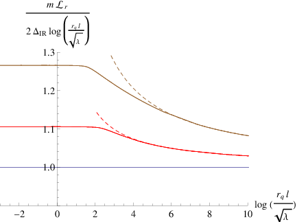
When the distance is large the theory reaches a new conformal point. Accordingly, the two-point function should behave again as a power law. Notice, however, that the conformal dimension in the IR of an operator dual to a particle of mass is different from the UV value (9.12). Indeed, in the IR the conformal dimension for an operator of mass is the one corresponding to the unflavored ABJM theory,
| (9.13) |
where and are given, respectively, in (2.3) and (2.4). Actually, one can check that and that for large values of the deformation parameter . The calculation of the two-point function in the IR limit of large is performed in detail in Appendix E, with the result:
| (9.14) |
where is a constant whose analytic expression is written in (E.35). Notice that due to our choice of the constant in (9.10), which corresponds to imposing the canonical normalization (9.11) to the two-point function in the UV regime.
The results obtained by the numerical evaluation of the integral (9.10) interpolate smoothly between the conformal behaviors (9.11) and (9.14). This is shown in Fig. 8, where we plot as a function of . For small values of the curve asymptotes to the ratio of conformal dimensions, in agreement with (9.11), whereas for large we recover the IR behavior (9.14).
10 Meson spectrum
Let us now test the flow encoded in our geometry by analyzing the mass spectrum of bound states. We will loosely refer to these bound states as mesons, although our background is not confining and quarkonia would be a more appropriate name for them. To carry out our analysis we will introduce additional external quarks, with a mass not necessarily equal to the mass of the quarks which backreact on the geometry. To distinguish between the two types of flavors we will call valence quarks to the additional ones, whereas the unquenched dynamical flavors of the geometry will be referred to as sea quarks. The ratio of the masses of the two types of quarks will be an important quantity in what follows. Indeed, is the natural parameter for the holographic renormalization group trajectory. When is large (small) we expect to reach a UV (IR) conformal fixed point, whereas for intermediate values of this mass ratio the theory should flow in such a way that the screening effects produced by the sea quarks decrease as we move towards the IR.
Within the context of the gauge/gravity duality, the valence quarks can be introduced by adding an additional flavor D6-brane, which will be treated as a probe in the backreacted geometry. The mesonic mass spectrum can be obtained from the normalizable fluctuations of the D6-brane probe. The way in which the D6-brane probe is embedded in the ten-dimensional geometry preserving the supersymmetry of the background can be determined by using kappa symmetry. For fixed values of the Minkowski and holographic coordinates, the D6-brane extends over a cycle inside the which has two directions along the base and one direction along the fiber. In order to specify further this configuration, let us parameterize the left invariant one-forms of the four-sphere metric (2.7) in terms of three angles , and ,
| (10.1) |
with , , . Then, our D6-brane probe will be extended along the Minkowski directions and embedded in the geometry in such a way that the angles and are constant and that the angle of the fiber depends on the holographic variable . The pullbacks (denoted by a hat) of the left-invariant one-forms (10.1) are and . The kappa symmetric configurations are those for which the function satisfies the first order BPS equation [23]:
| (10.2) |
which can be integrated as:
| (10.3) |
Here is the minimum value of the variable for the embedding, i.e., the value of for the tip of the brane. This minimum value of the coordinate for the embedding is related to the mass of the valence quarks introduced by the flavor probe. Indeed, by computing the Nambu-Goto action of a fundamental string stretched in the holographic direction between and we obtain as:
| (10.4) |
In the following we will take the Regge slope . Moreover, to simplify the description of the embedding, let us introduce the angular coordinate , defined as follows:
| (10.5) |
and let us define new angles and as:
| (10.6) |
where is the angle in (2.9). One can check that the ranges of the new angular variables are , . We will take the following set of worldvolume coordinates for the D6-brane:
| (10.7) |
Then, it is straightforward to verify that the induced metric on the D6-brane worldvolume takes the form:
| (10.8) |
We will restrict ourselves to study a particular set of fluctuations of the D6-brane probe, namely the fluctuations of the worldvolume gauge field . The equation for these fluctuations is:
| (10.9) |
where is the induced metric (10.8). More concretely, we will study this equation for the following ansatz for :
| (10.10) |
where is a constant polarization vector and denote the components along the angular directions. These modes are dual to the vector mesons of the theory, with being the momentum of the meson (, with being the mass of the meson). The non-vanishing components of the field strength are:
| (10.11) |
The fluctuation equation (10.9) is trivially satisfied when , whereas for it is satisfied if the polarization is transverse:
| (10.12) |
Moreover, by taking in (10.9) we arrive at the following differential equation for the radial function :
| (10.13) |

The mass levels correspond to the values of for which there are normalizable solutions of (10.13). They can be obtained numerically by the shooting technique. One gets in this way a discrete spectrum depending on a quantization number (, ). The numerical results for the first three levels are shown in Fig. 9 as functions of the mass ratio . One notices in these results that the meson masses increase as we move from the IR () to the UV (). This non-trivial flow is due to the vacuum polarization effects of the sea quarks, which are enhanced as we move towards the UV and the sea quarks become effectively massless. This is the expected behavior of bound state masses for a theory in the Coulomb phase, since the screening effects reduce effectively the strength of the quark-antiquark force.
One can get a very accurate description of the flow by applying the WKB approximation. The detailed calculation is presented in Appendix F. The WKB formula for the mass spectrum is:
| (10.14) |
where is the following integral:
| (10.15) |
The WKB mass levels (10.14) are compared with those obtained by the shooting technique in Fig. 9. We notice from these plots that the estimate (10.14) describes rather well the numerical results along the flow. Moreover, we can use the UV and IR limits of the functions and to obtain the asymptotic form of the WKB spectrum at the endpoints of the flow. This analysis is performed in detail in Appendix F (see eqs. (F.14) and (F.20)). As expected, in the deep IR the mass levels coincide with those of the unflavored ABJM model. In this latter model the mass spectrum of vector mesons can be computed analytically since the fluctuation equation can be solved in terms of hypergeometric functions [12, 13]. When the meson masses coincide with those obtained for the massless flavored model of [23].
We can use the WKB formulas (F.14) and (F.20) for the spectrum at the endpoints of the renormalization group flow to estimate the variation generated in the meson masses by changing the sea quark mass and switching on and off gradually the screening effects. It is interesting to point out that, within the WKB approximation, the ratio of these masses only depends on the number of flavors, and is given by:
| (10.16) |
where is the screening function defined in (8.13). As expected, when the right-hand side of (10.16) is equal to one, i.e., there is no variation of the masses along the flow. On the contrary, when the UV/IR mass ratio in (10.16) is always greater than one, which means that the masses grow as we move towards the UV and the screening effects become more important. In Appendix F we have expanded (10.16) for low values of the deformation parameter (see (F.21)). Moreover, for large the UV/IR mass ratio grows as (see (F.22) for the explicit formula).
11 Summary and conclusions
In this paper we obtained a holographic dual to Chern-Simons matter theory with unquenched flavor in the strongly-coupled Veneziano limit. The flavor degrees of freedom were added by a set of D6-branes smeared along the internal directions, which backreacted on the geometry by squashing it, while preserving supersymmetry. We considered massive flavors and found a non-trivial holographic renormalization group flow connecting two scale-invariant fixed points: the unflavored ABJM theory at the IR and the massless flavored model at the UV.
The quark mass played an important role as a control parameter of the solution. By increasing our solutions became closer to the unflavored ABJM model and we smoothly connected the unquenched flavored model to the ABJM theory without fundamentals. After this soft introduction of flavor no pathological behavior was found. Indeed, our backgrounds had good IR and UV behaviors, contrary to what happens to other models with unquenched flavor [22]. This made the ABJM model especially adequate to analyze the effects of unquenched fundamental matter in a holographic setup.
We analyzed different flavor effects in our model. In general, the screening effects due to loops of fundamentals were controlled by the relative value of the quark mass with respect to the characteristic length scale of the observable. If was small, which corresponds to the UV regime, the flavor effects were important, whereas they were suppressed if is large, i.e., at the IR. Among the different observables that we analyzed, the holographic entanglement entropy for a disk was specially appropriate since it counts precisely the effective number of degrees of freedom which are relevant at the length scale given by the radius of the disk. By using the refined entanglement entropy introduced in [26], we explicitly obtained the running of and verified the reduction of the number of degrees at the IR that was mentioned above. The other observables studied also supported this picture.
We end this paper with a short discussion on the outlook. We are convinced that our model could serve as a starting point to gain new insights on the effects of unquenched flavor in other holographic setups. One possible generalization could be the construction of a black hole for the unquenched massive flavor. Such a background could serve to study the meson melting phase transition which occurs when the tip of the brane approaches the horizon. This system was studied in [16], in the case in which the massive flavors are quenched and the corresponding flavor brane is a probe. Another possibility would be trying to find a gravity dual of a theory in which the sum of the two Chern-Simons levels is non-vanishing. According to [41] we should find a flavored solution of type IIA supergravity with non-zero Romans mass.
Our program is also to converge toward increasingly realistic holographic condensed matter models capable of testable predictions. To make contact with any condensed matter system, one is forced to consider non-vanishing components of the gauge field in the background or at the probe level. A natural flow of ideas taking one to land in the former case typically requires a deep understanding of the probe brane dynamics with worldvolume gauge fields turned on. As an initial step in this direction, we have started exploring what physical phenomena we will encompass by turning on a charge density, magnetic field, and internal flux on the worldvolume of an additional probe D6-brane. The variety of different phenomena seems incredibly rich, much in parallel with recent works on the D3-D7’ system [42] and the closely related D2-D8’ system [43]. Our findings will be reported elsewhere.
Acknowledgments
We are grateful to Daniel Areán, Manuel Asorey, Jose Ignacio Latorre, David Mateos, Carlos Núñez, and Ángel Paredes for useful discussions. The works of Y. B., N. J., and A. V. R. are funded in part by the Spanish grant FPA2011-22594, by Xunta de Galicia (Consellería de Educación, grant INCITE09 206 121 PR and grant PGIDIT10PXIB206075PR), by the Consolider-Ingenio 2010 Programme CPAN (CSD2007-00042), and by FEDER. The work of E.C. is partially supported by IISN - Belgium (conventions 4.4511.06 and 4.4514.08), by the “Communauté Française de Belgique” through the ARC program and by the ERC through the “SyDuGraM” Advanced Grant. Y. B. is supported by the Spanish FPU fellowship FPU12/00481. N. J. is supported also through the Juan de la Cierva program. N. J. and A. V. R. wish to thank Centro de Ciencias de Benasque Pedro Pascual and N. J. the Kavli IPMU for warm hospitalities while this work was in progress.
Appendix A BPS equations
In this Appendix we will derive the master equation (3.10), as well as the equations that allow to construct the metric and dilaton from the master function (i.e., (3.11), (3.12), and (3.13)).
Let us begin by writing the BPS equations that guarantee the preservation of SUSY. They can be written in terms of the function introduced in [23], which is defined as the following combination of the dilaton and the warp factor:
| (A.1) |
Then, it was proved in [23] that , , and are solutions to the following system of first-order differential equations:
| (A.2) |
Moreover, the warp factor can be recovered from , , and through:
| (A.3) |
where is an integration constant. Given and , the dilaton is obtained from (A.1). The function of the RR four-form can be related to the other functions of the background by using (3.6). Alternatively, can be obtained from the BPS system as:
| (A.4) |
In terms of the variable defined in (3.7), the BPS system (A.2) becomes:
| (A.5) |
In order to reduce this system, let us define as in [23] the functions and ,
| (A.6) |
Then, one can easily show that and satisfy the system:
| (A.7) |
whereas can be obtained from and by integrating the equation:
| (A.8) |
Let us next define the master function as in (3.9). One immediately verifies that, in terms of the functions and , this definition is equivalent to
| (A.9) |
By computing the derivative of (A.9) and using the BPS system (A.7), one can easily prove that:
| (A.10) |
From (A.10) one immediately finds:
| (A.11) |
where the prime denotes derivative with respect to . Moreover, from the BPS system we can calculate the derivative of and write the result as:
| (A.12) |
Plugging (A.11) into (A.12), we arrive at the following second-order equation for :
| (A.13) |
which can be straightforwardly shown to be equivalent to the master equation (3.10).
Let us see now how one can reconstruct the full solution from the knowledge of the function . First of all, we notice that from the expression of in (A.9), we get:
| (A.14) |
By combining this expression with (A.11) we obtain and :
| (A.15) |
By noticing that we arrive at the representation of the squashing function written in (3.14). Moreover, by using this result in (A.8), we obtain the differential equation satisfied by :
| (A.16) |
which allows to obtain once is known. The result of this integration is just the expression written in (3.11). Moreover, taking into account the expression of the squashing factor we get precisely the expression of written in (3.11).
Let us now compute by using and (A.11). We get:
| (A.17) |
and, after using (3.11), we arrive at:
| (A.18) |
By using this result and (3.11) in (A.3), we get that the warp factor can be written as in (3.12). The expression (3.13) for the dilaton is just a consequence of the definition of in (A.1) and of (A.18).
A.1 Equations of motion
Let us now verify that the first-order BPS system (A.2) implies the second-order equations of motion for the different fields. Let us work in Einstein frame and write the total action as:
| (A.19) |
where the action of type IIA supergravity is given by:
| (A.20) |
and the source contribution is the DBI+WZ action for the set of smeared D6-branes. Let us write this last action as in [23]. First of all, we introduce a charge distribution three-form . Then, the DBI+WZ action is given by:
| (A.21) |
where the DBI term has been written in terms of the so-called calibration form (denoted by ), whose pullback to the worldvolume is equal to the induced volume form for the supersymmetric embeddings. The expression of has been written in [23]. Let us reproduce it here for completeness:
| (A.22) |
where the ’s are the one-forms of the basis corresponding to the forms (2.11) and (2.14) (see [23] for further details). Notice that the equation of motion for derived from (A.19) is just . Therefore, the for our ansatz can be read from the right-hand side of (3.5).
The Maxwell equations for the forms and derived from (A.19) are:
| (A.23) |
while the equation for the dilaton is:
| (A.24) |
One can verify that, for our ansatz, (A.23) and (A.24) are a consequence of the BPS equations (A.2). To carry out this verification we need to know the radial derivatives of and (which are not written in (A.2)). The derivative of can be related to the derivative of ,
| (A.25) |
The radial derivative of the dilaton can be put in terms of the derivative of and by using (A.1):
| (A.26) |
It remains to check Einstein equations, which read:
| (A.27) |
where is the stress-energy tensor for the flavor branes, which is defined as:
| (A.28) |
In order to write the explicit expression for derived from the definition (A.28), let us introduce the following operation for any two -forms and :
| (A.29) |
Then, by computing explicitly the derivative of the action (A.21) with respect to the metric, one can check that:
| (A.30) |
It is now straightforward to compute explicitly the different components of this tensor. Written in flat components in the basis in which the calibration form has the form (A.22), we get:55 5 As compared to the case studied in [23], now we have terms proportional to that were absent for massless flavors.
| (A.31) |
By using these values one can verify that, the Einstein equations (A.27) are indeed satisfied as a consequence of the first-order system (A.2). Notice that, for the massive flavored background of Section 6, (and, therefore, ) has a finite discontinuity at . It follows from (A.27) that the Ricci tensor has also a finite jump at this point.
Appendix B Mass corrections in the UV
In this appendix we show how to obtain the first corrections to the conformal behavior of the metric and the dilaton from the UV asymptotic expansion of the master function written in (6.10). First we notice that the ratio can be written in terms of as:
| (B.1) |
leading to a useful identity:
| (B.2) |
Inserting the unit written in this way in the integral appearing in the expression of in (5.7), we get:
| (B.3) |
where is the following constant integral (depending on ):
| (B.4) |
and is the function
| (B.5) |
Using these results, we can immediately write:
| (B.6) |
The function can be easily expanded for large . At first non-trivial order we get:
| (B.7) |
Using that, for large ,
| (B.8) |
we easily arrive at the expansion of written in (6.16). Let us next find the large expansion for , which can be obtained by using the expansion of and in the relation . We get:
| (B.9) |
where the coefficient is given by:
| (B.10) |
It is straightforward to demonstrate that (B.10) coincides with the value of written in (6.17).
Let us now analyze the UV expansion of . First, we evaluate the integral appearing in (3.12):
| (B.11) |
By combining this result with the expansions (6.16) and (6.12) we get:
| (B.12) |
where is the UV AdS radius (3.39) and the coefficient is:
| (B.13) |
One can readily check that the prefactor in (B.12) coincides with the one in (6.18) and that the coefficient written in (B.13) is the same as the one in (6.19).
Let us now obtain the UV expansion of the function , defined in (A.1), which can be written as:
| (B.14) |
The UV expansion of this expression is:
| (B.15) |
where the coefficient can be written in terms of as:
| (B.16) |
By using the value of in (6.17), we can find a more explicit expression for :
| (B.17) |
Let us next obtain the expansion of by using . We get:
| (B.18) |
where the prefactor is
| (B.19) |
and can be shown to be the same as the asymptotic value of the dilaton written in (3.41). The coefficient is:
| (B.20) |
which has been written more explicitly in (6.19).
Finally, let us write these results in terms of the variable. At next-to-leading order, the relation between the coordinates and is obtained by integrating the differential equation:
| (B.21) |
We get:
| (B.22) |
This relation can be inverted as:
| (B.23) |
By plugging the expansion (B.23) into (6.16) and (6.18) one easily arrives at (6.22) and (6.23).
Appendix C More on the entanglement entropy
Let us study analytically the entanglement entropy and the function near the UV fixed point at . We shall represent in terms of a local functional as:
| (C.1) |
We will use this representation to compute the first-order variation of when the background functions and and the embedding function are varied around their UV values:
| (C.2) |
where , and is the function written in (7.23). At first order the corrections and can be parameterized as:
| (C.3) |
The constants and in (C.3) can be related to the ones characterizing the behavior of the background at the UV:
| (C.4) |
It is useful to define the following combination of and :
| (C.5) |
The perturbation of the profile is the correction, at first-order, of the solution of (7.7) which satisfies . By computing the first variation of (7.7) we find that is solution to the following second-order inhomogeneous differential equation:
| (C.6) |
More explicitly, after using the UV values of , , and , the differential equation (C.6) can be written as:
| (C.7) |
Let us next calculate the first-order variation of the entanglement entropy. From (C.1) we get:
| (C.8) |
where is defined as:
| (C.9) |
Using the explicit form of we get:
| (C.10) |
and it follows that:
| (C.11) |
Therefore, the lower limit contribution to the last term in (C.8) vanishes. Let us now study the contribution to this term of the limit. We will now check that decreases as in such a way that:
| (C.12) |
Thus, the upper limit of the last term in (C.8) also vanishes. To prove (C.12) we have to integrate the differential equation (C.7) and extract the large behavior of the solution. Amazingly, (C.7) can be integrated analytically. Its general solution can be written as the sum of two terms:
| (C.13) |
where is a particular solution of the equation and is a general solution of the homogeneous part of (C.7). We have found a particular solution , which can be written in terms of hypergeometric functions and is given by:
| (C.14) |
We are only interested in the behavior of for large . It is straightforward to prove that, for large , can be approximated as:
| (C.15) |
Thus, as for large ,
| (C.16) |
The general solution of the homogeneous differential equation which vanishes as is:
| (C.17) |
where is an arbitrary constant. For large the function in (C.17) behaves as:
| (C.18) |
Therefore,
| (C.19) |
Then, eq. (C.12) holds and the last term in (C.8) does not contribute to , as claimed above. Let us now calculate the other two contributions. First of all, the term due to the variation of is given by:
| (C.20) |
which, after using (7.24) to eliminate , becomes:
| (C.21) |
Similarly,
| (C.22) |
which, after eliminating , gives:
| (C.23) |
Thus, can be written as:
| (C.24) |
where is the constant defined in (C.5). Using the definition (7.20), it follows that the change in the function is:
| (C.25) |
Taking into account (7.11) and (7.14) this expression can be written as:
| (C.26) |
Therefore, we can write the function near the UV fixed point as:
| (C.27) |
where the constant coefficient can be read from (C.26),
| (C.28) |
Eq. (C.27) coincides with (7.31) when the former is written in terms of the dimension of the quark-antiquark bilinear operator in the massless flavored theory. Moreover, as is always positive, the sign of depends on the sign of the coefficient . We have checked that is negative for all values of the deformation parameter , in agreement with the expectation that is maximized at the UV fixed point.
C.1 Entanglement entropy on the strip
Let us now evaluate the entanglement entropy in the case in which the region is the strip of width in the -plane (see Fig. 10). In this case we consider a constant time surface , whose embedding in the ten-dimensional space is determined by a function . The induced metric on is,
| (C.29) |
where denotes the derivative of the holographic coordinate with respect to the cartesian coordinate and the function has been defined in (7.4). The entropy functional for the strip of width is given by:
| (C.30) |
where is the volume of the internal manifold, whose value was given after (7.6), is the function defined in (7.5), and is the length of the strip. As the integrand in does not depend on the coordinate , the corresponding Euler-Lagrange equation admits the following first integral:

| (C.31) |
or, more explicitly,
| (C.32) |
where and is the holographic coordinate of the turning point. It follows from this last expression that is given by:
| (C.33) |
Therefore, the width of the strip is given by the integral:
| (C.34) |
and the entropy is:
| (C.35) |
The integral (C.35) for is divergent in the UV. Indeed, from the behavior of the functions and at large (eqs. (7.10) and (7.11)), it follows that, when , the integrand in (C.35) behaves as:
| (C.36) |
and therefore diverges as , where is the upper limit of the integral, which can be regarded as a UV cutoff. More explicitly, one can rearrange the integral in (C.35) as:
| (C.37) |
where the divergent term is explicitly shown. We now define the rescaled functions and as:
| (C.38) |
Then, the finite term in can be written as:
| (C.39) |
whereas the divergent term takes the form:
| (C.40) |

We have evaluated numerically the right-hand side of (C.39) as a function of the strip width . The result is displayed in Fig. 11. One notices from these results that is negative and diverges as for small , where is a constant. Actually, for small the surface is in the UV region of the geometry and one can evaluate the entropy analytically in this limit. This is the subject of the next subsection, where we show that the constant is proportional to the free energy on the three-sphere of the massless flavored theory (see eq. (C.51) below). The analytical UV calculation is compared to the numerical results in Fig. 11.
C.1.1 UV limit
In order to study the UV limit it is convenient to change variables in the integrals (C.34) and (C.39). Let us introduce a new variable , related to as . Then, can be represented as:
| (C.41) |
while is given by:
| (C.42) |
Let us now obtain the expressions of and in the limit in which . In this case the argument of the functions and in the integrals is always large and one can take , . We get:
| (C.43) |
where is the following integral:
| (C.44) |
Using (C.44) in (C.43), we get:
| (C.45) |
Similarly, the finite part of the entropy is:
| (C.46) |
where is the integral:
| (C.47) |
Plugging (C.47) into (C.46), we arrive at:
| (C.48) |
Eliminating in favor of , we get:
| (C.49) |
However, from the definition of and in (7.11) it follows that:
| (C.50) |
where is the free energy of the massless flavored theory on the three sphere (see (7.17)). It follows that:
| (C.51) |
which is the result we were looking for. From the comparison of Fig. 11 to the numerical results we conclude that (C.51) is a good description of the entropy in the small region. Notice that the coefficient of on the right-hand side of (C.51) is determined by the free energy of the massless flavored theory. This is expected on general grounds in the UV region, since the masses of the quarks can be neglected in the high-energy regime.
C.1.2 IR limit
Let us now evaluate in the regime in which is large. In this case the surface penetrates deeply in the bulk and its tip is near the origin (i.e., is small). We will proceed as in Section 7.2 and split the interval in the integrals (C.34) and (C.39) as , where is considered small enough so that one can use the unflavored background functions in the interval . Moreover, when with , and one can neglect the terms containing in the integrals. Then, the strip width can be approximated as:
| (C.52) |
When, and we can extend the first integral in (C.52) up to and neglect the contribution of the second integral (which is proportional to ). Then, can be approximately written as:
| (C.53) |
and, as expected, a small value of leads to a large value of . Similarly, we can perform the same type of manipulations in the expression (C.39) of . We find:
| (C.54) |
Performing the first integral in (C.54) in the limit for fixed , we arrive at:
| (C.55) |
where is the constant:
| (C.56) |
We can now eliminate in (C.55) the turning point in favor of by using (C.53). We find:
| (C.57) |
where we have written the result in terms of . The first term in (C.57) is just the strip entanglement entropy for the unflavored theory. The constant represents the asymptotic value of as . One can approximate this constant by taking in (C.56). After using (7.14) to relate and to , we arrive at:
| (C.58) |
Appendix D Asymptotic quark-antiquark potential
The purpose of this appendix is to obtain the analytic expressions for the potential energy in the UV and IR limit. We will start by calculating the leading and subleading UV potential.
D.1 UV potential
Let us find the approximate value of the potential in the case in which the distance is small and the hanging string only explores the UV of the geometry. This is equivalent to considering the limit in which the turning point is large. It is then more convenient to perform a change of variables in the integrals (8.6) and (8.10) and write and as:
| (D.1) |
We want to compute the leading value of , as well as the first deviation from the conformal behavior. For this reason we will make use of the asymptotic expressions of the different functions of the metric derived in Section 6.1.
Let us begin by computing the integrals in (D.1) in a power series expansion for large . From (6.16) and (6.18) we get:
| (D.2) |
where and are given in (6.17) and (6.19) and has been defined in (6.15). Then, it follows that:
| (D.3) |
Using these results we obtain the following expansion of the separation :
| (D.4) |
where is the integral (C.44), and and are:
| (D.5) |
where is the following ratio of Euler Gamma functions:
| (D.6) |
Using these results we arrive at:
| (D.7) |
Let us now compute the energy at leading and next-to-leading order in the UV (large or small ). First, we need the expansion:
| (D.8) |
Then, it is easy to verify that can be expanded as:
| (D.9) |
where is the integral (C.47) and and are:
| (D.10) |
To compute we also need as a function of . It follows from (B.22) that:
| (D.11) |
Then, one can check that:
| (D.12) |
Let us write as a function of the separation . For this purpose we have to eliminate in favor of . By inverting (D.7), we get:
| (D.13) |
Using this result, we get the following dependence of with the distance
| (D.14) |
where we have represented this relation in terms of the rescaled quantities and . Notice that the leading term (the first term on the right-hand side of (D.14)) is given by the potential of the massless flavored background, as expected.
D.2 IR potential
We now estimate the potential for large separations. In this case we will content ourselves to compute the leading order contribution. For large separations the hanging fundamental string penetrates deeply in the geometry, which is equivalent to saying that is small. We will follow an approach similar to the one in Sections 7.2 and C.1.2 and we will split the interval of the integrals (8.6) and (8.10) as with being small. We will assume that is small enough so that the background functions are well approximated by (7.32) in the interval . Then, we can estimate the integral (8.6) for as:
| (D.15) |
where is the unflavored radius (2.3) and we have used the fact that for we have that when and, therefore, in this interval we can neglect in the square root of the denominator of the integrand in (8.6). The first integral in (D.15) can be done analytically, yielding the result:
| (D.16) |
For small , at leading order, we get from (D.16):
| (D.17) |
which confirms that is large when is small. We can make similar approximations in the integral (8.10) with the result:
| (D.18) |
Performing explicitly the integral, we get:
| (D.19) |
which, at leading order, becomes:
| (D.20) |
Eliminating by using (D.17) we arrive at the estimate (8.14).
Appendix E Asymptotics of the two-point functions
In this appendix we study the renormalized geodesic distance, and the corresponding two-point function of bulk operators with large conformal dimensions, in the UV limit of small separation and in the IR regime in which . In the former case, our study will serve to fix the normalization constant of (9.10), as well as the analytic form of the correlator near the UV fixed point. This is the case we analyze first in the next subsection.
E.1 UV behavior
We will now obtain the form of the correlator in the UV limit in which the turning point is large and the geodesic does not penetrate much into the bulk of the geometry. In order to study this limiting case, it is convenient to perform a change of variables in the integral (9.7) and write it as:
| (E.1) |
Similarly, the renormalized geodesic length can be represented as:
| (E.2) |
where . When is large the argument of the functions in the integrals (E.1) and (E.2) is large and one can use the UV asymptotic expressions (6.18) and (7.10). Therefore, we can approximate as:
| (E.3) |
The integral in (E.3) just gives and, thus, we have:
| (E.4) |
It follows that, when is large is small. Thus the UV limit we are studying corresponds to . Similarly, the UV limit of is:
| (E.5) |
The integral in this last equation is:
| (E.6) |
On the other hand, the UV conformal dimension of a bulk field of mass has been written in (9.12). Taking these facts into account, we can write:
| (E.7) |
If the operator is canonically normalized in the short-distance limit, the coefficient in the numerator of (E.7) should be chosen to be one as in (9.11). Therefore, it follows that the constant is fixed to
| (E.8) |
Let us now evaluate the first correction of the two-point correlator around the UV fixed point. Let us expand the function for large as in (C.2) and (C.3). Then, for large we get:
| (E.9) |
where . Similarly:
| (E.10) |
It follows that the separation of the two points of the correlator can be written as:
| (E.11) |
where and are the following integrals:
| (E.12) |
Let us invert the relation (E.11) at first order and write as a function of . We get:
| (E.13) |
where is a constant given by:
| (E.14) |
Moreover, the renormalized geodesic length at first order takes the form:
| (E.15) |
where is the integral defined in (E.12) and is:
| (E.16) |
Let us now write in terms of . By using (E.13) to eliminate in terms of we arrive at:
| (E.17) |
where the coefficient is given by:
| (E.18) |
Therefore, the two-point correlator near the UV fixed point can be written as:
| (E.19) |
where the function parameterizes the deviation from the conformal behavior near the UV fixed point and is given, at first order, by
| (E.20) |
where the new constant is just:
| (E.21) |
E.2 IR behavior
Let us now analyze the two-point functions in the IR limit, which corresponds to taking . In this case the geodesic penetrates deeply in the bulk. We will proceed similarly to what we did in Section D.2 for the potential in the IR. Accordingly, we split the interval as for some small. Near the turning point, i.e., when , we can approximate the functions and as:
| (E.22) |
where is the AdS radius of the unflavored ABJM solution and and are the parameters of the unflavored running solution. It follows that, in this IR region, the function behaves as:
| (E.23) |
Moreover, the dilaton is constant and given by the ABJM value written in (2.4).
Suppose that we have chosen some . Let us then split the integral (9.7) for as:
| (E.24) |
where should be sent to at the end of the calculation. Let us approximate the first integral in (E.24) by taking the functions in the deep IR, as in (E.22). We obtain:
| (E.25) |
For small we can approximate this integral as:
| (E.26) |
To evaluate approximately we notice that and, therefore, it is large for . Then, we can neglect the one inside the square root and approximate as:
| (E.27) |
Since the integral in (E.27) converges and is independent of , it follows that and, therefore, it can be neglected with respect to the large value of . Thus, we take
| (E.28) |
Notice that it follows from this equation that is large if is small, as it should be in the IR regime. Let us next perform a similar analysis for the renormalized geodesic length . First, we consider the IR integral:
| (E.29) |
To evaluate the UV integral we proceed similarly to what we did for the integral for and, in this case, we only keep the one inside the square root. Then:
| (E.30) |
Therefore:
| (E.31) |
where is the conformal dimension of the operator in the IR conformal point, given by:
| (E.32) |
which is just (9.13). Let us next define the following quantities:
| (E.33) |
Then, after using the relation (E.28) to eliminate in favor of , we get:
| (E.34) |
Then, it follows that the IR limit of the two-point correlator is as in (9.14), where is the normalization constant given by:
| (E.35) |
It turns out that, in the expression of the integrals in (E.33) we can take the limits (in ) and (in ). Actually, it can be easily proved that, after taking these limits, and can be recast as:
| (E.36) |
Notice that the form of the correlator is consistent with the fact that the conformal symmetry is recovered in the IR limit . The non-canonical normalization factor is due to the fact that we chose to renormalize in such a way that the correlator is canonically normalized in the opposite UV limit .
Appendix F WKB mass levels
Consider the following differential equation for the function :
| (F.1) |
where takes values in the range , is the mass parameter and and are two arbitrary functions that are independent of . We will assume that near these functions behave as:
| (F.2) |
where , , , and are constants. By a of suitable change of variables, the differential equation (F.1) can be converted into a Schrödinger equation, which only admits a discrete set of normalizable solutions for a set of values of parameterized by a quantum number . The mass levels for large values of can be evaluated in the WKB approximation [44], with the result:
| (F.3) |
where is the integral:
| (F.4) |
In our case, the functions and which correspond to the fluctuation equation (10.13) are:
| (F.5) |
and it is immediate to extract the exponents , , , and :
| (F.6) |
Using these values one immediately finds that the WKB mass levels are given by (10.14).
F.1 Asymptotic spectra
Let us now evaluate analytically the meson spectrum in the two limiting cases in which the sea quark mass is small or large compared to the valence quark mass . Notice that (see eqs. (5.6) and (5.7)). Therefore, (10.4) can be regarded as giving the relation as a function of .
Let us consider first the case in which is small. Clearly, when for fixed one necessarily must have large. Actually, integrating (10.4) by using the asymptotic expression of written in (6.16) at leading order, we get:
| (F.7) |
where the constant has been defined in (6.15). Thus, when for fixed the coordinate of the tip of the flavor brane increases as:
| (F.8) |
Let us now evaluate when is large. First of all we perform a change of variables in the integral (10.15) and rewrite as:
| (F.9) |
If is large, the argument of the functions and in (F.9) is large and we can use their UV asymptotic expressions (6.16) and (6.18) to evaluate them. At leading order, we get:
| (F.10) |
where is the value of the coordinate corresponding to . Therefore, for for fixed the is approximately
| (F.11) |
Using this result in (10.14) we get the following mass spectrum in the UV limit:
| (F.12) |
Let us write this result in terms of physical quantities. Recall that and are related to the ’t Hooft coupling and to the valence quark mass as:
| (F.13) |
where is the screening function written in (8.13). Then, for large , we have:
| (F.14) |
where we have taken . Eq. (F.14) is exactly the WKB mass spectrum one gets for vector mesons in the massless flavored background of ref. [23].
Let us next consider the limit in which is small. Since , it follows from (10.4) that must be small. Actually, we can estimate the relation between and by extracting from (4.9) and (5.6) the approximate expression of near . We get:
| (F.15) |
Then, we have:
| (F.16) |
and it follows that, for fixed and large , the coordinate of the tip of the flavor brane behaves as:
| (F.17) |
Thus, for large sea quark mass and thus the dynamics of the fluctuating flavor brane is dominated by the IR, where the solution corresponds to the running solution of the unflavored system. In this case, we have at leading order near :
| (F.18) |
where, in the last step, we used that . Thus,
| (F.19) |
and, after evaluating the integral (F.9) and writing the result in terms of the ’t Hooft coupling and the valence quark mass , we have:
| (F.20) |
which is exactly the mass spectrum of vector mesons in the unflavored ABJM model [13]. By combining (F.14) and (F.20) we obtain the UV/IR mass relation written in (10.16). It is now straightforward to obtain this ratio for small and large values of the deformation parameter. Indeed, for small one can expand as:
| (F.21) |
Moreover, in the opposite limit in which is very large, we have:
| (F.22) |
References
- [1] O. Aharony, O. Bergman, D. L. Jafferis and J. M. Maldacena, “N=6 superconformal Chern-Simons-matter theories, M2-branes and their gravity duals,” JHEP 0810, 091 (2008) [arXiv:0806.1218 [hep-th]].
- [2] J. M. Maldacena, “The large limit of superconformal field theories and supergravity”, Adv. Theor. Math. Phys. 2 (1998) 231, hep-th/9711200.
- [3] O. Aharony, S. S. Gubser, J. M. Maldacena, H. Ooguri and Y. Oz, “Large N field theories, string theory and gravity,” Phys. Rept. 323, 183 (2000) [arXiv:hep-th/9905111].
- [4] J. Bagger, N. Lambert, “Modeling Multiple M2’s,” Phys. Rev. D75, 045020 (2007) [hep-th/0611108]; “Gauge symmetry and supersymmetry of multiple M2-branes,” Phys. Rev. D77 (2008) 065008 [arXiv:0711.0955 [hep-th]]; “Comments on multiple M2-branes,” JHEP 0802, 105 (2008) [arXiv:0712.3738 [hep-th]].
- [5] A. Gustavsson, “Algebraic structures on parallel M2-branes,” Nucl. Phys. B811, 66-76 (2009) [arXiv:0709.1260 [hep-th]].
- [6] I. R. Klebanov and G. Torri, “M2-branes and AdS/CFT,” Int. J. Mod. Phys. A 25, 332 (2010) [arXiv:0909.1580 [hep-th]].
- [7] T. Klose, “Review of AdS/CFT Integrability, Chapter IV.3: N=6 Chern-Simons and Strings on AdS4xCP3,” Lett. Math. Phys. 99, 401 (2012) [arXiv:1012.3999 [hep-th]].
- [8] M. Mariño, “Lectures on localization and matrix models in supersymmetric Chern-Simons-matter theories,” J. Phys. A 44, 463001 (2011) [arXiv:1104.0783 [hep-th]].
- [9] J. Bagger, N. Lambert, S. Mukhi and C. Papageorgakis, “Multiple Membranes in M-theory,” arXiv:1203.3546 [hep-th].
- [10] S. Hohenegger, I. Kirsch, “A Note on the holography of Chern-Simons matter theories with flavour,” JHEP 0904, 129 (2009) [arXiv:0903.1730 [hep-th]].
- [11] D. Gaiotto, D. L. Jafferis, “Notes on adding D6 branes wrapping RP**3 in AdS(4) x CP**3,” [arXiv:0903.2175 [hep-th]].
- [12] Y. Hikida, W. Li, T. Takayanagi, “ABJM with Flavors and FQHE,” JHEP 0907, 065 (2009) [arXiv:0903.2194 [hep-th]].
- [13] K. Jensen, “More Holographic Berezinskii-Kosterlitz-Thouless Transitions,” Phys. Rev. D82, 046005 (2010) [arXiv:1006.3066 [hep-th]].
- [14] M. Ammon, J. Erdmenger, R. Meyer et al., “Adding Flavor to AdS(4)/CFT(3),” JHEP 0911, 125 (2009) [arXiv:0909.3845 [hep-th]].
- [15] G. Zafrir, “Embedding massive flavor in ABJM,” JHEP 1210 (2012) 056 [arXiv:1202.4295 [hep-th]].
- [16] N. Jokela, J. Mas, A. V. Ramallo and D. Zoakos, “Thermodynamics of the brane in Chern-Simons matter theories with flavor,” JHEP 1302 (2013) 144 [arXiv:1211.0630 [hep-th]].
- [17] F. Bigazzi, R. Casero, A. L. Cotrone, E. Kiritsis, A. Paredes, “Non-critical holography and four-dimensional CFT’s with fundamentals,” JHEP 0510, 012 (2005) [hep-th/0505140].
- [18] G. Veneziano, “Some Aspects Of A Unified Approach To Gauge, Dual And Gribov Theories,” Nucl. Phys. B 117, 519 (1976).
- [19] R. Casero, C. Nunez, A. Paredes, “Towards the string dual of N=1 SQCD-like theories,” Phys. Rev. D73, 086005 (2006) [hep-th/0602027]; “Elaborations on the String Dual to N=1 SQCD,” Phys. Rev. D77, 046003 (2008) [arXiv:0709.3421 [hep-th]]; C. Hoyos-Badajoz, C. Nunez and I. Papadimitriou, “Comments on the String dual to N=1 SQCD,” Phys. Rev. D 78, 086005 (2008) [arXiv:0807.3039 [hep-th]]; E. Conde, J. Gaillard and A. V. Ramallo, “On the holographic dual of N=1 SQCD with massive flavors,” JHEP 1110, 023 (2011) [arXiv:1107.3803 [hep-th]].
- [20] F. Benini, F. Canoura, S. Cremonesi, C. Nunez, A. V. Ramallo, “Unquenched flavors in the Klebanov-Witten model,” JHEP 0702, 090 (2007) [hep-th/0612118]; “Backreacting flavors in the Klebanov-Strassler background,” JHEP 0709 (2007) 109 [arXiv:0706.1238 [hep-th]]; M. Ihl, A. Kundu and S. Kundu, “Back-reaction of Non-supersymmetric Probes: Phase Transition and Stability,” arXiv:1208.2663 [hep-th].
- [21] F. Bigazzi, A. L. Cotrone, J. Mas, A. Paredes, A. V. Ramallo, J. Tarrio, “D3-D7 Quark-Gluon Plasmas,” JHEP 0911, 117 (2009) [arXiv:0909.2865 [hep-th]]; F. Bigazzi, A. L. Cotrone, J. Tarrio, “Hydrodynamics of fundamental matter,” JHEP 1002, 083 (2010) [arXiv:0912.3256 [hep-th]]; F. Bigazzi, A. L. Cotrone, J. Mas, D. Mayerson, J. Tarrio, “D3-D7 Quark-Gluon Plasmas at Finite Baryon Density,” JHEP 1104, 060 (2011) [arXiv:1101.3560 [hep-th]]; A. Magaña, J. Mas, L. Mazzanti and J. Tarrio, “Probes on D3-D7 Quark-Gluon Plasmas,” JHEP 1207, 058 (2012) [arXiv:1205.6176 [hep-th]].
- [22] C. Nunez, A. Paredes, A. V. Ramallo, “Unquenched flavor in the gauge/gravity correspondence,” Adv. High Energy Phys. 2010, 196714 (2010) [arXiv:1002.1088 [hep-th]].
- [23] E. Conde and A. V. Ramallo, “On the gravity dual of Chern-Simons-matter theories with unquenched flavor,” JHEP 1107, 099 (2011) [arXiv:1105.6045 [hep-th]].
- [24] M. S. Bianchi, S. Penati, M. Siani, “Infrared stability of ABJ-like theories,” JHEP 1001, 080 (2010) [arXiv:0910.5200 [hep-th]]; M. S. Bianchi, S. Penati, M. Siani, “Infrared Stability of N = 2 Chern-Simons Matter Theories,” JHEP 1005, 106 (2010) [arXiv:0912.4282 [hep-th]].
- [25] S. Ryu and T. Takayanagi, “Holographic derivation of entanglement entropy from AdS/CFT,” Phys. Rev. Lett. 96 (2006) 181602 [arXiv:hep-th/0603001]; “Aspects of holographic entanglement entropy,” JHEP 0608 (2006) 045 [arXiv:hep-th/0605073].
- [26] H. Liu and M. Mezei, “A Refinement of entanglement entropy and the number of degrees of freedom,” arXiv:1202.2070 [hep-th].
- [27] R. C. Myers and A. Sinha, “Holographic c-theorems in arbitrary dimensions,” JHEP 1101, 125 (2011) [arXiv:1011.5819 [hep-th]]; “Seeing a c-theorem with holography,” Phys. Rev. D 82 (2010) 046006 [arXiv:1006.1263 [hep-th]]; D. L. Jafferis, I. R. Klebanov, S. S. Pufu and B. R. Safdi, “Towards the F-Theorem: N=2 Field Theories on the Three-Sphere,” JHEP 1106 (2011) 102 [arXiv:1103.1181 [hep-th]]; I. R. Klebanov, S. S. Pufu and B. R. Safdi, “F-Theorem without Supersymmetry,” JHEP 1110 (2011) 038 [arXiv:1105.4598 [hep-th]]; “Entanglement Entropy of 3-d Conformal Gauge Theories with Many Flavors,” JHEP 1205 (2012) 036 [arXiv:1112.5342 [hep-th]].
- [28] H. Casini and M. Huerta, “On the RG running of the entanglement entropy of a circle,” Phys. Rev. D 85 (2012) 125016 [arXiv:1202.5650 [hep-th]].
- [29] R. L. Bryant and S. Salamon, “On the construction of some complete metrics with exceptional holonomy”, Duke Math. J. 58, 829 (1989); G. W. Gibbons, D. N. Page and C. N. Pope, “Einstein metrics on , and bundles”, Commun. Math. Phys. 127, 529 (1990).
- [30] M. Atiyah and E. Witten, “M theory dynamics on a manifold of G(2) holonomy,” Adv. Theor. Math. Phys. 6 (2003) 1 [hep-th/0107177].
- [31] R. Emparan, C. V. Johnson and R. C. Myers, “Surface terms as counterterms in the AdS / CFT correspondence,” Phys. Rev. D 60 (1999) 104001 [hep-th/9903238].
- [32] H. Casini, M. Huerta and R. C. Myers, “Towards a derivation of holographic entanglement entropy,” JHEP 1105, 036 (2011) [arXiv:1102.0440 [hep-th]].
- [33] H. Liu and M. Mezei, “Probing renormalization group flows using entanglement entropy,” arXiv:1309.6935 [hep-th].
- [34] A. Kitaev and J. Preskill, “Topological entanglement entropy,” Phys. Rev. Lett. 96 (2006) 110404 [hep-th/0510092].
- [35] M. Levin and X. -G. Wen, “Detecting Topological Order in a Ground State Wave Function,” Phys. Rev. Lett. 96 (2006) 110405.
- [36] J. M. Maldacena, “Wilson loops in large N field theories,” Phys. Rev. Lett. 80, 4859 (1998) [arXiv:hep-th/9803002].
- [37] S. J. Rey and J. T. Yee, “Macroscopic strings as heavy quarks in large N gauge theory and anti-de Sitter supergravity,” Eur. Phys. J. C 22 (2001) 379 [arXiv:hep-th/9803001].
- [38] V. Balasubramanian and S. F. Ross, “Holographic particle detection,” Phys. Rev. D 61 (2000) 044007 [hep-th/9906226].
- [39] J. Louko, D. Marolf and S. F. Ross, “On geodesic propagators and black hole holography,” Phys. Rev. D 62 (2000) 044041 [hep-th/0002111].
- [40] P. Kraus, H. Ooguri and S. Shenker, “Inside the horizon with AdS / CFT,” Phys. Rev. D 67 (2003) 124022 [hep-th/0212277].
- [41] D. Gaiotto, A. Tomasiello, “The gauge dual of Romans mass,” JHEP 1001, 015 (2010). [arXiv:0901.0969 [hep-th]; “Perturbing gauge/gravity duals by a Romans mass,” J. Phys. A A42, 465205 (2009). [arXiv:0904.3959 [hep-th]].
- [42] O. Bergman, N. Jokela, G. Lifschytz and M. Lippert, “Quantum Hall Effect in a Holographic Model,” JHEP 1010 (2010) 063 [arXiv:1003.4965 [hep-th]]; “Striped instability of a holographic Fermi-like liquid,” JHEP 1110 (2011) 034 [arXiv:1106.3883 [hep-th]]; N. Jokela, G. Lifschytz and M. Lippert, “Magneto-roton excitation in a holographic quantum Hall fluid,” JHEP 1102 (2011) 104 [arXiv:1012.1230 [hep-th]]; “Magnetic effects in a holographic Fermi-like liquid,” JHEP 1205 (2012) 105 [arXiv:1204.3914 [hep-th]]; “Holographic anyonic superfluidity,” arXiv:1307.6336 [hep-th].
- [43] N. Jokela, M. Järvinen and M. Lippert, “A holographic quantum Hall model at integer filling,” JHEP 1105 (2011) 101 [arXiv:1101.3329 [hep-th]]; “Fluctuations of a holographic quantum Hall fluid,” JHEP 1201 (2012) 072 [arXiv:1107.3836 [hep-th]]; “Fluctuations and instabilities of a holographic metal,” JHEP 1302 (2013) 007 [arXiv:1211.1381 [hep-th]].
- [44] J. G. Russo and K. Sfetsos, “Rotating D3-branes and QCD in three dimensions”, Adv. Theor. Math. Phys. 3(1999) 131, hep-th/9901056.