跳到论文正文
W Papers独立论文阅读器 arXiv:1309.4401 论文正文 计算阅读时间 · 0%
引用这篇论文根据当前论文元数据生成,正式投稿前建议核对。


License: arXiv.org perpetual non-exclusive license
arXiv:1309.4401v2 [hep-th] 14 Nov 2013

Electrostatic Interaction due to Patch Potentials on Smooth Conducting Surfaces

César D. Fosco1,2 Affiliation: 1 Centro Atómico Bariloche, Comisión Nacional de Energía Atómica, R8402AGP Bariloche, Argentina    Fernando C. Lombardo3 Affiliation: 1 Centro Atómico Bariloche, Comisión Nacional de Energía Atómica, R8402AGP Bariloche, Argentina    Francisco D. Mazzitelli1,2 Affiliation: 1 Centro Atómico Bariloche, Comisión Nacional de Energía Atómica, R8402AGP Bariloche, Argentina Affiliation: 2 Instituto Balseiro, Universidad Nacional de Cuyo, R8402AGP Bariloche, Argentina Affiliation: 3 Departamento de Física Juan José Giambiagi, FCEyN UBA, Facultad de Ciencias Exactas y Naturales, Ciudad Universitaria, Pabellón I, 1428 Buenos Aires, Argentina - IFIBA
today
Abstract

We evaluate the electrostatic interaction energy between two surfaces, one flat and the other slightly curved, in terms of the two-point autocorrelation functions for patch potentials on each one of them, and of a single function ψ\psi which defines the curved surface. The resulting interaction energy, a functional of ψ\psi, is evaluated up to the second order in a derivative expansion approach. We derive explicit formulae for the coefficients of that expansion as simple integrals involving the autocorrelation functions, and evaluate them for some relevant patch-potential profiles and geometries.

I Introduction

Mostly because of the ever improving precision achieved by Casimir force experiments [1], it has become important to be able to discriminate that force from other interactions which, under some circumstances, may even mask it completely. Among them, the most relevant ones are usually electrostatic in nature. Indeed, in the usual experimental setup one deals with metallic mirrors which, even if electrically neutral, may still produce relevant residual effects. Surface imperfections can lead to a local departure from ideal metallic behaviour, yielding space-dependent ‘patch’ potentials on the mirrors’ surfaces. Those potentials, which may be interpreted as due to the existence of superficial dipole layers on otherwise neutral bodies [2], can indeed produce a force. This force may be relevant in precision experiments related to many different areas of physics [3, 4].

For the case of two infinite parallel planes, that force has been studied in detail by Speake and Trenkle in Ref.[5]. The force is, naturally, a function of aa, the distance between the mirrors, and of the patch potentials on the surfaces. It has been shown, however, that the force depends on the potentials only through their autocorrelation functions. A conceptually different situation, which however leads to a formally identical result corresponds to random potentials. In those cases, the correlation functions is all the information we have about the underlying potentials.

Recent Casimir effect experiments do involve, however, different geometries. Of particular interest is the case of a sphere in front of a plane; the influence of patch potentials in Casimir measurements for this geometry has been recently analyzed in Ref.[6], using a Proximity Force Approximation (PFA) [7]. The same system has also been studied by using an exact numerical approach [8]. The PFA approach amounts, in this context, to a local application of the parallel plate result, and may therefore be implemented based in the results of Ref.[5].

It is the aim of this paper to go beyond the PFA, by extending the results for the patch potentials force, known for parallel planes, to a class of different geometries, namely, to the case of an infinite plane facing a slightly curved surface. By the latter we mean a surface which curvature radius is much larger than the distance between the surfaces. Moreover, we know that in this situation the Casimir interaction may be calculated using a Derivative Expansion (DE) approach [9], of which the Proximity Force Approximation (PFA) is the leading term. We shall construct here the same approximation for the patch potentials force, namely, the first nontrivial correction to the PFA.

With the extra requirement that the autocorrelation lengths should also be smaller than the curvature radius of the curved surface, we shall be able to apply here essentially the same approach used in the Casimir case to the calculation of the leading and subleading terms for the patch potential electrostatic interaction. The leading term will of course amount to the well-known PFA, while the subleading one shall account for the first correction to it.

To be more precise about the system that we consider, it will consist of two static surfaces, denoted by LL and RR, embedded in 33-dimensional space. LL shall be assumed to be flat, and, by a proper choice of coordinates, to coincide with the x3=0x_{3}=0 plane (x1x_{1}, x2x_{2} and x3x_{3} denote the three Cartesian coordinates of a point 𝐱{\mathbf{x}} in this coordinate system). The RR surface is, on the other hand, assumed to be definable by a single function, namely, by an equation of the form x3=ψ⁡(𝐱∥)x_{3}=\psi({\mathbf{x}_{\parallel}}), where 𝐱∥=(x1,x2){\mathbf{x}_{\parallel}}=(x_{1},x_{2}). This assumption does not cover all the possible curved surfaces; however, it is sufficiently general as to describe the usually considered experimental setups. As advanced, the RR surface will be assumed to be smooth, something that will be quantified below in terms of ψ\psi, its derivatives, and the correlation lengths characterizing the patch potentials. The extension to the case of two slightly deformed surfaces is straightforward.

In a previous work [10], dealing with a DE approach to the electrostatic interaction between perfect conductors, we analyzed what may be regarded as a limiting case of a system with patch potentials. Namely, one in which the surfaces LL and RR are held at constant potentials, so that there is a constant electrostatic potential difference VV between them. There, at second order, the DE of the electrostatic energy UD​EU_{DE} stored between the surfaces was found to be:

UD​E=ϵ0​V22​∫d2​𝐱∥​1ψ​[1+13​(∇ψ)2].U_{DE}=\frac{\epsilon_{0}V^{2}}{2}\int d^{2}{\mathbf{x}_{\parallel}}\,\frac{1}{\psi}\left[1+\frac{1}{3}(\nabla\psi)^{2}\right]\;. (1)

On the other hand (for a system with the same geometry) in the presence of patch potentials, on general grounds we expect a DE expansion (up to the same order) to have the form:

UD​E=ϵ02​∫d2​𝐱∥​[V⁡(ψ)+Z⁡(ψ)​(∇ψ)2],U_{DE}=\frac{\epsilon_{0}}{2}\int d^{2}{\mathbf{x}_{\parallel}}\,\left[V(\psi)+Z(\psi)(\nabla\psi)^{2}\right]\,, (2)

where V⁡(ψ)V(\psi) and Z⁡(ψ)Z(\psi) are functions that depend on the shape of the RR surface and on the correlation functions for the patch potentials on both surfaces. One of our main goals in this paper is to find an explicit expression for the function Z⁡(ψ)Z(\psi) (the zeroth-order, PFA contribution has already been computed in previous works).

This paper is organized as follows: in Section II, we obtain a formal general expression for the electrostatic interaction energy between the two surfaces, in terms of the correlation function between the patch potentials, and of the exact Dirichlet Green’s function for the spatial region delimited by the two surfaces. Based on that formal expression we obtain, in Section III, the electrostatic interaction energy for small departures from the parallel planes case. In Section IV, we use those results to expand the interaction energy up to the second order in derivatives, and apply the results to different geometries and different models for the correlation functions of the patch potentials. Our final remarks are included in Section V. The Appendix contain some details of the expansion of the Green’s function for almost flat surfaces.

II Interaction energy

In order to obtain the interaction energy, we calculate the electrostatic potential φ\varphi, solution to an electrostatic problem in the region 𝒱{\mathcal{V}}, limited by the surfaces LL and RR, namely, 0≤x3≤ψ⁡(𝐱∥)0\leq x_{3}\leq\psi({\mathbf{x}_{\parallel}}). A proper definition of the problem requires some care, since one wants to consider the seemingly inconsistent situation of having space dependent potentials on the surfaces of conducting bodies. We bypass that problem by following the approach of Ref.[5], where the conflicting conditions are introduced on (infinitesimally close) different surfaces. More concretely, the electrostatic problem is defined for the volume 𝒱{\mathcal{V}}, with Dirichlet type boundary conditions on the LL and RR surfaces. Patch potentials are then introduced not on LL and RR, but on two slightly shifted surfaces, LδL_{\delta} and RδR_{\delta}, defined by x3=δx_{3}=\delta and x3=ψ⁡(𝐱∥)−δx_{3}=\psi({\mathbf{x}_{\parallel}})-\delta (δ>0\delta>0), respectively. Potentials are not introduced as boundary conditions (they have already been defined on LL are RR); rather, one models them by means of two electric dipole layers with surface densities 𝐦L,R​(𝐱∥)=mL,R​(𝐱∥)​𝐧^L,R{\mathbf{m}_{L,R}}(\mathbf{x}_{\parallel})=m_{L,R}(\mathbf{x}_{\parallel})\mathbf{\hat{n}}_{L,R}, (𝐧^L,R\mathbf{\hat{n}}_{L,R}: unit normal to the respective surface).

In the limit when the layers are adjacent to the surfaces, those moment distributions generate variations in the surface potentials, determined by two functions, φL,R​(𝐱∥)=mL,R​(𝐱∥)/ϵ0\varphi_{L,R}({\mathbf{x}_{\parallel}})=m_{L,R}(\mathbf{x}_{\parallel})/\epsilon_{0}, which indeed do fix the potential φ\varphi on the inner face of LL and RR, respectively.

Thus, the electrostatic problem amounts to one where the charge density inside 𝒱{\mathcal{V}} (associated to the dipole layers above) is given by:

ρ⁡(𝐱)=ϵ0​[φL​(𝐱∥)​𝐧^L⋅∇δ​(x3−δ)+φR​(𝐱∥)​𝐧^R⋅∇δ​(x3−ψ⁡(𝐱∥)+δ)],\rho({\mathbf{x}})=\epsilon_{0}\Big[\varphi_{L}({\mathbf{x}_{\parallel}})\,{\mathbf{\hat{n}}}_{L}\cdot\nabla\delta(x_{3}-\delta)+\varphi_{R}({\mathbf{x}_{\parallel}})\,{\mathbf{\hat{n}}}_{R}\cdot\nabla\delta(x_{3}-\psi({\mathbf{x}_{\parallel}})+\delta)\Big]\;, (3)

where δ→0\delta\to 0, the limit whereby the dipole layers approach the two surfaces ‘from inside’ shall be taken when deriving the expression for the energy (see below).

The energy UU may be written in terms of the scalar potential φ⁡(𝐱)\varphi({\mathbf{x}}), as follows:

U=ϵ02​∫𝒱d3​𝐱​(∇φ​(𝐱))2.U\,=\,\frac{\epsilon_{0}}{2}\int_{\mathcal{V}}d^{3}{\mathbf{x}}\,({\mathbf{\nabla}}\varphi({\mathbf{x}}))^{2}\;. (4)

To proceed, we need to write UU in terms of φL\varphi_{L} and φR\varphi_{R}. The formal solution for φ\varphi inside 𝒱{\mathcal{V}} may be written in terms of the Dirichlet Green’s function G⁡(𝐱,𝐲)G({\mathbf{x}},{\mathbf{y}}), defined for 𝐱{\mathbf{x}} and 𝐲{\mathbf{y}} in 𝒱{\mathcal{V}}, as follows:

φ⁡(𝐱)=1ϵ0​∫𝐱′∈𝒱G⁡(𝐱,𝐱′)​ρ​(𝐱′).\varphi({\mathbf{x}})\;=\;\frac{1}{\epsilon_{0}}\int_{{\mathbf{x}^{\prime}}\in\mathcal{V}}G({\mathbf{x}},{\mathbf{x}^{\prime}})\rho({\mathbf{x}^{\prime}})\,. (5)

In our conventions, GG is determined by the equations:

−∇𝐱2​G​(𝐱,𝐲)=δ⁡(𝐱−𝐲),G⁡(𝐱,𝐲)= 0,∀𝐱∈𝒱,∀𝐲∈𝒮=L∪R.-\nabla^{2}_{\mathbf{x}}G({\mathbf{x}},{\mathbf{y}})\;=\;\delta({\mathbf{x}}-{\mathbf{y}})\;\;,\;\;\;G({\mathbf{x}},{\mathbf{y}})\;=\;0\;,\;\;\forall{\mathbf{x}}\in{\mathcal{V}}\;,\;\;\forall{\mathbf{y}}\in{\mathcal{S}}=L\cup R\;. (6)

Besides, the Dirichlet Green’s function is symmetric: G⁡(𝐱,𝐲)=G⁡(𝐲,𝐱)G({\mathbf{x}},{\mathbf{y}})=G({\mathbf{y}},{\mathbf{x}}).

Inserting Eq.(3) into Eq.(5), we obtain

φ(𝐱)=−∮𝐱′∈𝒮δdσ′φ(𝐱′)∂∂n′G(𝐱,𝐱′)\varphi({\mathbf{x}})\;=\;-\,\oint_{{\mathbf{x}^{\prime}}\in\mathcal{\mathcal{S}}_{\delta}}d\sigma^{\prime}\,{\varphi}({\mathbf{x}^{\prime}})\,\frac{\partial}{\partial n^{\prime}}G({\mathbf{x}},{\mathbf{x}^{\prime}}) (7)

where 𝒮δ≡Lδ∪Rδ{\mathcal{S}_{\delta}}\equiv L_{\delta}\cup R_{\delta} denotes the surfaces of the two layers, and ∂∂n′\frac{\partial}{\partial n^{\prime}} is the directional derivative along the outer normal to 𝒮δ{\mathcal{S}_{\delta}} at each point on the surface, and d​σ′d\sigma^{\prime} is the surface element at each point 𝐱′∈𝒮δ{\mathbf{x}^{\prime}}\in{\mathcal{S}}_{\delta}. Note that the r.h.s. of the equation above is completely determined by the prescribed values φL,R{\varphi}_{L,R} of the patch potentials on LδL_{\delta} and RδR_{\delta}.

Inserting now (7) into (4), integrating by parts, using (6), and then letting δ→0\delta\to 0, we see that UU may be written as follows:

U=ϵ02​∮𝒮d​σ′​∮𝒮d​σ′′​φ​(𝐱′)​𝒦​(𝐱′,𝐱′′)​φ​(𝐱′′),U\;=\;\frac{\epsilon_{0}}{2}\,\oint_{\mathcal{S}}d\sigma^{\prime}\oint_{\mathcal{S}}d\sigma^{\prime\prime}\;\varphi({\mathbf{x}^{\prime}})\,{\mathcal{K}}({\mathbf{x}^{\prime}},{\mathbf{x}^{\prime\prime}})\,\varphi({\mathbf{x}^{\prime\prime}})\;, (8)

where we have removed the δ\delta subscript for the surfaces since the δ→0\delta\to 0 has been taken. The kernel 𝒦{\mathcal{K}} is constructed in terms of the normal derivatives of the exact Green’s function GG on 𝒮{\mathcal{S}}:

𝒦⁡(𝐱′,𝐱′′)=∂n′∂n′′G⁡(𝐱′,𝐱′′),𝐱′,𝐱′′∈𝒮.{\mathcal{K}}({\mathbf{x}^{\prime}},{\mathbf{x}^{\prime\prime}})\,=\,\partial_{n^{\prime}}\partial_{n^{\prime\prime}}G({\mathbf{x}^{\prime}},{\mathbf{x}^{\prime\prime}})\;,\;\;{\mathbf{x}^{\prime}},\,{\mathbf{x}^{\prime\prime}}\in{\mathcal{S}}\;. (9)

Note that the presence of the metallic media has been taken into account, by discarding boundary terms which involve the values of the Green’s function on those media. At this point the distinction between 𝒮{\mathcal{S}} and 𝒮δ{\mathcal{S}}_{\delta} ceases to be necessary, since we have ended up with an expression where one has to integrate on the inner faces of the mirrors only.

Expression (8) has to be now particularized to the case of the region we are considering, and the assumed values for the potential on the boundary. Denoting by 𝒦A​B{\mathcal{K}}_{AB}, A,B=L,RA,B=L,R the special form adopted by the kernel 𝒦{\mathcal{K}} when its first argument belong to the surface AA and its second argument to BB, we see that:

U=∑A,BUA​BU\;=\;\sum_{A,B}\,U_{AB} (10)

where:

UL​L\displaystyle U_{LL} =\displaystyle= ϵ02​∫d2​𝐱∥′​∫d2​𝐱∥′′​φL​(𝐱∥′)​𝒦L​L​(𝐱∥′,𝐱∥′′)​φL​(𝐱∥′′)\displaystyle\frac{\epsilon_{0}}{2}\,\int d^{2}{\mathbf{x}_{\parallel}^{\prime}}\int d^{2}{\mathbf{x}_{\parallel}^{\prime\prime}}\;\varphi_{L}({\mathbf{x}_{\parallel}^{\prime}})\,{\mathcal{K}}_{LL}({\mathbf{x}_{\parallel}^{\prime}},{\mathbf{x}_{\parallel}^{\prime\prime}})\,\varphi_{L}({\mathbf{x}_{\parallel}^{\prime\prime}})
UL​R\displaystyle U_{LR} =\displaystyle= ϵ02​∫d2​𝐱∥′​∫d2​𝐱∥′′​g⁡(𝐱∥′′)​φL​(𝐱∥′)​𝒦L​R​(𝐱∥′,𝐱∥′′)​φR​(𝐱∥′′)\displaystyle\frac{\epsilon_{0}}{2}\,\int d^{2}{\mathbf{x}_{\parallel}^{\prime}}\int d^{2}{\mathbf{x}_{\parallel}^{\prime\prime}}\sqrt{g({\mathbf{x}_{\parallel}^{\prime\prime}})}\;\varphi_{L}({\mathbf{x}_{\parallel}^{\prime}})\,{\mathcal{K}}_{LR}({\mathbf{x}_{\parallel}^{\prime}},{\mathbf{x}_{\parallel}^{\prime\prime}})\,\varphi_{R}({\mathbf{x}_{\parallel}^{\prime\prime}})
UR​L\displaystyle U_{RL} =\displaystyle= ϵ02​∫d2​𝐱∥′​∫d2​𝐱∥′′​g⁡(𝐱∥′)​φR​(𝐱∥′)​𝒦R​L​(𝐱∥′,𝐱∥′′)​φL​(𝐱∥′′)\displaystyle\frac{\epsilon_{0}}{2}\,\int d^{2}{\mathbf{x}_{\parallel}^{\prime}}\int d^{2}{\mathbf{x}_{\parallel}^{\prime\prime}}\,\sqrt{g({\mathbf{x}_{\parallel}^{\prime}})}\,\varphi_{R}({\mathbf{x}_{\parallel}^{\prime}})\,{\mathcal{K}}_{RL}({\mathbf{x}_{\parallel}^{\prime}},{\mathbf{x}_{\parallel}^{\prime\prime}})\,\varphi_{L}({\mathbf{x}_{\parallel}^{\prime\prime}})
UR​R\displaystyle U_{RR} =\displaystyle= ϵ02​∫d2​𝐱∥′​∫d2​𝐱∥′′​g⁡(𝐱∥′)​g⁡(𝐱∥′′)​φR​(𝐱∥′)​𝒦R​R​(𝐱∥′,𝐱∥′′)​φR​(𝐱∥′′),\displaystyle\frac{\epsilon_{0}}{2}\,\int d^{2}{\mathbf{x}_{\parallel}^{\prime}}\int d^{2}{\mathbf{x}_{\parallel}^{\prime\prime}}\sqrt{g({\mathbf{x}_{\parallel}^{\prime}})}\sqrt{g({\mathbf{x}_{\parallel}^{\prime\prime}})}\,\varphi_{R}({\mathbf{x}_{\parallel}^{\prime}})\,{\mathcal{K}}_{RR}({\mathbf{x}_{\parallel}^{\prime}},{\mathbf{x}_{\parallel}^{\prime\prime}})\,\varphi_{R}({\mathbf{x}_{\parallel}^{\prime\prime}})\;, (11)

where we have written the area element in terms of the parametrization of the respective surface, namely, on LL, d2​σ=d2​𝐱∥d^{2}\sigma=d^{2}{\mathbf{x}_{\parallel}}, while on RR: d2​σ=d2​𝐱∥​1+(∇ψ​(𝐱∥))2d^{2}\sigma=d^{2}{\mathbf{x}_{\parallel}}\sqrt{1+(\nabla\psi({\mathbf{x}_{\parallel}}))^{2}}.

The explicit form of the outer normal derivative depends on the surface, LL or RR, considered. For LL, we have ∂n=−∂3\partial_{n}=-\partial_{3} while for RR:

∂n=∂3−(∂iψ)∂i1+(∇ψ​(𝐱∥))2,\partial_{n}=\frac{\partial_{3}-(\partial_{i}\psi)\partial_{i}}{\sqrt{1+(\nabla\psi({\mathbf{x}_{\parallel}}))^{2}}}\;, (12)

where ii and, in what follows, indices from the middle of the Roman alphabet (i,j,…)(i,\,j,\,\ldots) run from 11 to 22.

We may write then a more explicit form for UA​BU_{AB}, as follows:

UL​L\displaystyle U_{LL} =\displaystyle= ϵ02​∫𝐱∥′,𝐱∥′′[∂3′∂3′′G⁡(𝐱′,𝐱′′)]x3′=x3′′=0​φL​(𝐱∥′′)​φL​(𝐱∥′)\displaystyle\frac{\epsilon_{0}}{2}\,\int_{{\mathbf{x}_{\parallel}^{\prime}},{\mathbf{x}_{\parallel}^{\prime\prime}}}\;\big[\partial^{\prime}_{3}\partial^{\prime\prime}_{3}G({\mathbf{x}^{\prime}},{\mathbf{x}^{\prime\prime}})\big]_{x^{\prime}_{3}=x^{\prime\prime}_{3}=0}\varphi_{L}({\mathbf{x}_{\parallel}^{\prime\prime}})\varphi_{L}({\mathbf{x}_{\parallel}^{\prime}})
UL​R\displaystyle U_{LR} =\displaystyle= −ϵ02∫𝐱∥′,𝐱∥′′[∂3′(∂3′′−∂i′′ψ∂i′′)G(𝐱′,𝐱′′)]x3′=0,x3′′=ψ⁡(𝐱∥′′)φR(𝐱∥′′)φL(𝐱∥′)\displaystyle-\frac{\epsilon_{0}}{2}\,\int_{{\mathbf{x}_{\parallel}^{\prime}},{\mathbf{x}_{\parallel}^{\prime\prime}}}\big[\partial^{\prime}_{3}(\partial^{\prime\prime}_{3}-\partial^{\prime\prime}_{i}\psi\partial^{\prime\prime}_{i})G({\mathbf{x}^{\prime}},{\mathbf{x}^{\prime\prime}})\big]_{x^{\prime}_{3}=0,x^{\prime\prime}_{3}=\psi({\mathbf{x}_{\parallel}^{\prime\prime}})}\varphi_{R}({\mathbf{x}_{\parallel}^{\prime\prime}})\varphi_{L}({\mathbf{x}_{\parallel}^{\prime}})
UR​L\displaystyle U_{RL} =\displaystyle= −ϵ02∫𝐱∥′,𝐱∥′′[(∂3′−∂i′ψ∂i′)∂3′′G(𝐱′,𝐱′′)]x3′=ψ⁡(𝐱∥′),x3′′=0φL(𝐱∥′′)φR(𝐱∥′)\displaystyle-\frac{\epsilon_{0}}{2}\,\int_{{\mathbf{x}_{\parallel}^{\prime}},{\mathbf{x}_{\parallel}^{\prime\prime}}}\big[(\partial^{\prime}_{3}-\partial^{\prime}_{i}\psi\partial^{\prime}_{i})\partial^{\prime\prime}_{3}G({\mathbf{x}^{\prime}},{\mathbf{x}^{\prime\prime}})\big]_{x^{\prime}_{3}=\psi({\mathbf{x}_{\parallel}^{\prime}}),x^{\prime\prime}_{3}=0}\varphi_{L}({\mathbf{x}_{\parallel}^{\prime\prime}})\varphi_{R}({\mathbf{x}_{\parallel}^{\prime}})
UR​R\displaystyle U_{RR} =\displaystyle= ϵ02∫𝐱∥′,𝐱∥′′[(∂3′−∂i′ψ∂i′)(∂3′′−∂j′′ψ∂j′′)G(𝐱′,𝐱′′)]x3′=ψ⁡(𝐱∥′),x3′′∈ψ⁡(𝐱∥′′)φR(𝐱∥′′)φR(𝐱∥′),\displaystyle\frac{\epsilon_{0}}{2}\,\int_{{\mathbf{x}_{\parallel}^{\prime}},{\mathbf{x}_{\parallel}^{\prime\prime}}}\big[(\partial^{\prime}_{3}-\partial^{\prime}_{i}\psi\partial^{\prime}_{i})(\partial^{\prime\prime}_{3}-\partial^{\prime\prime}_{j}\psi\partial^{\prime\prime}_{j})G({\mathbf{x}^{\prime}},{\mathbf{x}^{\prime\prime}})\big]_{x^{\prime}_{3}=\psi({\mathbf{x}_{\parallel}^{\prime}}),x^{\prime\prime}_{3}\in\psi({\mathbf{x}_{\parallel}^{\prime\prime}})}\varphi_{R}({\mathbf{x}_{\parallel}^{\prime\prime}})\varphi_{R}({\mathbf{x}_{\parallel}^{\prime}})\;, (13)

where the 1+(∇ψ​(𝐱∥))2\sqrt{1+(\nabla\psi({\mathbf{x}_{\parallel}}))^{2}} factors from the surface element on RR have been exactly cancelled with identical ones in the denominators of the normal derivatives. In order to simplify the expressions, in the equation above and in what follows we omit the integration measure and use the notation

∫d2𝐱∥′∫d2𝐱∥′′→∫𝐱∥′,𝐱∥′′.\int d^{2}{\mathbf{x}_{\parallel}^{\prime}}\int d^{2}{\mathbf{x}_{\parallel}^{\prime\prime}}\rightarrow\int_{{\mathbf{x}_{\parallel}^{\prime}},{\mathbf{x}_{\parallel}^{\prime\prime}}}\,\,\;. (14)

III Perturbative expansion

To obtain the DE, following the approach we introduced in previous references, we consider now the situation ψ⁡(𝐱∥)=a+η⁡(𝐱∥)\psi({\mathbf{x}_{\parallel}})=a+\eta({\mathbf{x}_{\parallel}}) with |η⁡(𝐱∥)|<<a|\eta({\mathbf{x}_{\parallel}})|<<a, and expand UU in powers of η\eta, up to the second order.

This expansion shall induce the corresponding expansion for UU,

U=U(0)+U(1)+U(2)+…U\;=\;U^{(0)}\,+\,U^{(1)}\,+\,U^{(2)}\,+\,\ldots (15)

where the index denotes the corresponding order in η\eta. Also, each order can be further decomposed, as follows:

U(α)=∑A,BUA,B(α).U^{(\alpha)}\;=\;\sum_{A,B}\,U^{(\alpha)}_{A,B}\;. (16)

The dependence on η\eta in each term of the sum above will come from the Green’s function dependence on ψ\psi, some details of which are presented in the Appendix. This shall produce different contributions to each order, which we will consider now in turn. For the η0\eta^{0} order, we have:

UL​L(0)=ϵ02​∫𝐱∥′,𝐱∥′′[∂3′∂3′′G(0)​(𝐱′,𝐱′′)]x3′=0,x3′′=0​φL​(𝐱∥′′)​φL​(𝐱∥′),U^{(0)}_{LL}\,=\,\frac{\epsilon_{0}}{2}\,\int_{{\mathbf{x}_{\parallel}^{\prime}},{\mathbf{x}_{\parallel}^{\prime\prime}}}\;\big[\partial^{\prime}_{3}\partial^{\prime\prime}_{3}G^{(0)}({\mathbf{x}^{\prime}},{\mathbf{x}^{\prime\prime}})\big]_{x^{\prime}_{3}=0,x^{\prime\prime}_{3}=0}\varphi_{L}({\mathbf{x}_{\parallel}^{\prime\prime}})\varphi_{L}({\mathbf{x}_{\parallel}^{\prime}})\;, (17)
UL​R(0)=−ϵ02∫𝐱∥′,𝐱∥′′[∂3′∂3′′G(0)(𝐱′,𝐱′′)]x3′=0,x3′′=aφR(𝐱∥′′)φL(𝐱∥′),U^{(0)}_{LR}\;=\;-\frac{\epsilon_{0}}{2}\,\int_{{\mathbf{x}_{\parallel}^{\prime}},{\mathbf{x}_{\parallel}^{\prime\prime}}}\big[\partial^{\prime}_{3}\partial^{\prime\prime}_{3}G^{(0)}({\mathbf{x}^{\prime}},{\mathbf{x}^{\prime\prime}})\big]_{x^{\prime}_{3}=0,x^{\prime\prime}_{3}=a}\varphi_{R}({\mathbf{x}_{\parallel}^{\prime\prime}})\varphi_{L}({\mathbf{x}_{\parallel}^{\prime}})\;, (18)
UR​L(0)=−ϵ02∫𝐱∥′,𝐱∥′′[∂3′∂3′′G(0)(𝐱′,𝐱′′)]x3′=a,x3′′=0φL(𝐱∥′′)φR(𝐱∥′)U^{(0)}_{RL}\;=\;-\frac{\epsilon_{0}}{2}\,\int_{{\mathbf{x}_{\parallel}^{\prime}},{\mathbf{x}_{\parallel}^{\prime\prime}}}\big[\partial^{\prime}_{3}\partial^{\prime\prime}_{3}G^{(0)}({\mathbf{x}^{\prime}},{\mathbf{x}^{\prime\prime}})\big]_{x^{\prime}_{3}=a,x^{\prime\prime}_{3}=0}\varphi_{L}({\mathbf{x}_{\parallel}^{\prime\prime}})\varphi_{R}({\mathbf{x}_{\parallel}^{\prime}}) (19)

and

UR​R(0)=ϵ02​∫𝐱∥′,𝐱∥′′[∂3′∂3′′G(0)​(𝐱′,𝐱′′)]x3′=a,x3′′=a​φR​(𝐱∥′′)​φR​(𝐱∥′).U^{(0)}_{RR}\;=\;\frac{\epsilon_{0}}{2}\,\int_{{\mathbf{x}_{\parallel}^{\prime}},{\mathbf{x}_{\parallel}^{\prime\prime}}}\big[\partial^{\prime}_{3}\partial^{\prime\prime}_{3}G^{(0)}({\mathbf{x}^{\prime}},{\mathbf{x}^{\prime\prime}})\big]_{x^{\prime}_{3}=a,x^{\prime\prime}_{3}=a}\varphi_{R}({\mathbf{x}_{\parallel}^{\prime\prime}})\varphi_{R}({\mathbf{x}_{\parallel}^{\prime}})\;. (20)

It is now convenient to note that, since the kernels depending on the 0t​h0^{th} order Green’s function are translation invariant along the parallel directions, they can only depend on the difference 𝐱∥′−𝐱∥′′{\mathbf{x}^{\prime}_{\parallel}}-{\mathbf{x}^{\prime\prime}_{\parallel}}. Thus, under a shift of arguments in the integrals, and defining 𝐲∥≡𝐱∥′′−𝐱∥′{\mathbf{y}_{\parallel}}\equiv{\mathbf{x}_{\parallel}^{\prime\prime}}-{\mathbf{x}_{\parallel}^{\prime}}, it is straightforward to see that the respective energies per unit area, 𝒰A​B(0)≡UA​B(0)/𝒜{\mathcal{U}}^{(0)}_{AB}\equiv U^{(0)}_{AB}/{\mathcal{A}} (where 𝒜{\mathcal{A}} is the area of the flat plate), can be written as follows:

𝒰L​L(0)=ϵ02​∫𝐲∥[∂3′∂3′′G(0)​(𝐱′,𝐱′′)]x3′=0,x3′′=0​ΩL​L​(𝐲∥),{\mathcal{U}}^{(0)}_{LL}\,=\,\frac{\epsilon_{0}}{2}\,\int_{{\mathbf{y}_{\parallel}}}\;\big[\partial^{\prime}_{3}\partial^{\prime\prime}_{3}G^{(0)}({\mathbf{x}^{\prime}},{\mathbf{x}^{\prime\prime}})\big]_{x^{\prime}_{3}=0,x^{\prime\prime}_{3}=0}\Omega_{LL}({\mathbf{y}_{\parallel}})\;, (21)
𝒰L​R(0)=−ϵ02∫𝐲∥[∂3′∂3′′G(0)(𝐱′,𝐱′′)]x3′=0,x3′′=aΩR​L(𝐲∥),{\mathcal{U}}^{(0)}_{LR}\;=\;-\frac{\epsilon_{0}}{2}\,\int_{\mathbf{y}_{\parallel}}\big[\partial^{\prime}_{3}\partial^{\prime\prime}_{3}G^{(0)}({\mathbf{x}^{\prime}},{\mathbf{x}^{\prime\prime}})\big]_{x^{\prime}_{3}=0,x^{\prime\prime}_{3}=a}\Omega_{RL}({\mathbf{y}_{\parallel}})\;, (22)
𝒰R​L(0)=−ϵ02∫𝐲∥[∂3′∂3′′G(0)(𝐱′,𝐱′′)]x3′=a,x3′′=0ΩL​R(𝐲∥){\mathcal{U}}^{(0)}_{RL}\;=\;-\frac{\epsilon_{0}}{2}\,\int_{\mathbf{y}_{\parallel}}\big[\partial^{\prime}_{3}\partial^{\prime\prime}_{3}G^{(0)}({\mathbf{x}^{\prime}},{\mathbf{x}^{\prime\prime}})\big]_{x^{\prime}_{3}=a,x^{\prime\prime}_{3}=0}\Omega_{LR}({\mathbf{y}_{\parallel}}) (23)
𝒰R​R(0)=ϵ02​∫𝐱∥′,𝐱∥′′[∂3′∂3′′G(0)​(𝐱′,𝐱′′)]x3′=a,x3′′=a​ΩR​R​(𝐲∥),{\mathcal{U}}^{(0)}_{RR}\;=\;\frac{\epsilon_{0}}{2}\,\int_{{\mathbf{x}_{\parallel}^{\prime}},{\mathbf{x}_{\parallel}^{\prime\prime}}}\big[\partial^{\prime}_{3}\partial^{\prime\prime}_{3}G^{(0)}({\mathbf{x}^{\prime}},{\mathbf{x}^{\prime\prime}})\big]_{x^{\prime}_{3}=a,x^{\prime\prime}_{3}=a}\Omega_{RR}({\mathbf{y}_{\parallel}})\;, (24)

where ΩA​B\Omega_{AB} denotes the correlation functions for the patch potentials, defined by:

ΩA​B​(𝐱∥)=1𝒜​∫d2​𝐳∥​φA​(𝐱∥+𝐳∥)​φB​(𝐳∥).\Omega_{AB}({\mathbf{x}_{\parallel}})\,=\,\frac{1}{\mathcal{A}}\int d^{2}{\mathbf{z}_{\parallel}}\;\varphi_{A}({\mathbf{x}_{\parallel}}+{\mathbf{z}_{\parallel}})\varphi_{B}({\mathbf{z}_{\parallel}})\;. (25)

Note that, because of the translation invariance, these contributions to the energy depends on the correlations, and not on the potentials themselves.

The leading term of the interaction energy can be obtained by evaluating the densities above in Fourier space. The result is

𝒰(0)\displaystyle{\mathcal{U}}^{(0)} =\displaystyle= −ϵ0∫d2​𝐤∥(2​π)2|𝐤∥|e2​|𝐤∥|​a−1(Ω~L​L(𝐤∥)+Ω~R​R(𝐤∥))\displaystyle-\epsilon_{0}\int\frac{d^{2}{\mathbf{k}_{\parallel}}}{(2\pi)^{2}}\,\frac{|{\mathbf{k}_{\parallel}}|}{e^{2|{\mathbf{k}_{\parallel}}|a}-1}\,\left({\widetilde{\Omega}}_{LL}({\mathbf{k}_{\parallel}})+{\widetilde{\Omega}}_{RR}({\mathbf{k}_{\parallel}})\right) (26)
+\displaystyle+ ϵ0​∫d2​𝐤∥(2​π)2​|𝐤∥|sinh⁡(|𝐤∥|​a)​Ω~L​R​(𝐤∥),\displaystyle\epsilon_{0}\int\frac{d^{2}{\mathbf{k}_{\parallel}}}{(2\pi)^{2}}\,\frac{|{\mathbf{k}_{\parallel}}|}{\sinh(|{\mathbf{k}_{\parallel}}|a)}\,{\widetilde{\Omega}}_{LR}({\mathbf{k}_{\parallel}})\;,

where we have used the symmetry Ω~L​R=Ω~R​L{\widetilde{\Omega}}_{LR}={\widetilde{\Omega}}_{RL}; besides, Ω~A​B{\widetilde{\Omega}}_{AB} is by construction a function of 𝐤∥{\mathbf{k}_{\parallel}}. It is worth mentioning at this point that an identical result would follow from the assumption of the existence of purely statistical correlations between the potentials.

The result of Eq.(26) coincides, up to terms independent of aa, with that of Ref. [5]. One could try to recover the usual result for perfect conductors assuming that φL=V\varphi_{L}=V and φR=0\varphi_{R}=0. In this case Eq.(26) gives 𝒰(0)=−ϵ0V2/(2a){\mathcal{U}}^{(0)}=-\epsilon_{0}V^{2}/(2a), i.e. the usual result for a capacitor with the opposite sign. This sign comes from the fact that we are computing the electrostatic energy for two grounded surfaces with dipole layers close to them, that we are modelling with the potentials φA\varphi_{A}. The case of two surfaces at different potentials has an additional surface term (discarded in the formal derivation of the previous section) that would reverse the sign in the final answer.

Regarding the η1\eta^{1} order, it is quite straightforward to see that it vanishes under the assumption that the spatial average of η\eta is zero. This will be enough for our purpose of computing the DE (see below).

Finally, let us consider now the second order contributions. We shall neglect here the ΩA≠B\Omega_{A\neq B} correlations, since they are assumed to be strongly suppressed with the distance between plates (at least in comparison with the autocorrelations ΩA=A\Omega_{A=A}). Thus we just need to compute:

UL​L(2)\displaystyle U^{(2)}_{LL} =\displaystyle= ϵ02​∫𝐱∥′,𝐱∥′′[∂3′∂3′′G⁡(𝐱′,𝐱′′)]x3′=x3′′=0(2)​φL​(𝐱∥′′)​φL​(𝐱∥′)\displaystyle\frac{\epsilon_{0}}{2}\,\int_{{\mathbf{x}_{\parallel}^{\prime}},{\mathbf{x}_{\parallel}^{\prime\prime}}}\;\big[\partial^{\prime}_{3}\partial^{\prime\prime}_{3}G({\mathbf{x}^{\prime}},{\mathbf{x}^{\prime\prime}})\big]_{x^{\prime}_{3}=x^{\prime\prime}_{3}=0}^{(2)}\varphi_{L}({\mathbf{x}_{\parallel}^{\prime\prime}})\varphi_{L}({\mathbf{x}_{\parallel}^{\prime}})
UR​R(2)\displaystyle U^{(2)}_{RR} =\displaystyle= ϵ02​∫𝐱∥′,𝐱∥′′[∂3′∂3′′G⁡(𝐱′,𝐱′′)]x3′=ψ⁡(𝐱∥′),x3′′=ψ⁡(𝐱∥′′)(2)​φR​(𝐱∥′′)​φR​(𝐱∥′)\displaystyle\frac{\epsilon_{0}}{2}\,\int_{{\mathbf{x}_{\parallel}^{\prime}},{\mathbf{x}_{\parallel}^{\prime\prime}}}\;\big[\partial^{\prime}_{3}\partial^{\prime\prime}_{3}G({\mathbf{x}^{\prime}},{\mathbf{x}^{\prime\prime}})\big]_{x^{\prime}_{3}=\psi({\mathbf{x}_{\parallel}^{\prime}}),x^{\prime\prime}_{3}=\psi({\mathbf{x}_{\parallel}^{\prime\prime}})}^{(2)}\,\varphi_{R}({\mathbf{x}_{\parallel}^{\prime\prime}})\varphi_{R}({\mathbf{x}_{\parallel}^{\prime}}) (27)

which depend on two second-order objects, determined by the Green’s functions.

To calculate this contribution we shall further assume that even when one of the surfaces is curved, the product of the two potentials is appreciably different from zero only when the distance between the two arguments is small. Assuming that this autocorrelation length is much smaller than the curvature radius, we shall still assume the translation invariance of the arguments in the Green’s function on that region. In this way, those contributions may be again written in terms of the autocorrelation functions, namely,

UL​L(2)\displaystyle U^{(2)}_{LL} =\displaystyle= ϵ02​∫𝐱∥′,𝐱∥′′[∂3′∂3′′G⁡(𝐱′,𝐱′′)]x3′=x3′′=0(2)​ΩL​L​(𝐱∥′′−𝐱∥′)\displaystyle\frac{\epsilon_{0}}{2}\,\int_{{\mathbf{x}_{\parallel}^{\prime}},{\mathbf{x}_{\parallel}^{\prime\prime}}}\;\big[\partial^{\prime}_{3}\partial^{\prime\prime}_{3}G({\mathbf{x}^{\prime}},{\mathbf{x}^{\prime\prime}})\big]_{x^{\prime}_{3}=x^{\prime\prime}_{3}=0}^{(2)}\Omega_{LL}({\mathbf{x}_{\parallel}^{\prime\prime}}-{\mathbf{x}_{\parallel}^{\prime}})
UR​R(2)\displaystyle U^{(2)}_{RR} =\displaystyle= ϵ02​∫𝐱∥′,𝐱∥′′[∂3′∂3′′G⁡(𝐱′,𝐱′′)]x3′=ψ⁡(𝐱∥′),x3′′=ψ⁡(𝐱∥′′)(2)​ΩR​R​(𝐱∥′′−𝐱∥′).\displaystyle\frac{\epsilon_{0}}{2}\,\int_{{\mathbf{x}_{\parallel}^{\prime}},{\mathbf{x}_{\parallel}^{\prime\prime}}}\;\big[\partial^{\prime}_{3}\partial^{\prime\prime}_{3}G({\mathbf{x}^{\prime}},{\mathbf{x}^{\prime\prime}})\big]_{x^{\prime}_{3}=\psi({\mathbf{x}_{\parallel}^{\prime}}),x^{\prime\prime}_{3}=\psi({\mathbf{x}_{\parallel}^{\prime\prime}})}^{(2)}\,\Omega_{RR}({\mathbf{x}_{\parallel}^{\prime\prime}}-{\mathbf{x}_{\parallel}^{\prime}})\;. (28)

Then, performing the expansion of the Green’s function, a rather lengthy but otherwise standard calculation shows that, for A=L,RA=L,R,

UA​A(2)=12​∫d2​𝐤∥(2​π)2​|η~​(𝐤∥)|2​fA​A​(𝐤∥),U^{(2)}_{AA}\;=\;\frac{1}{2}\,\int\frac{d^{2}{\mathbf{k}_{\parallel}}}{(2\pi)^{2}}\,\big|{\tilde{\eta}}({\mathbf{k}_{\parallel}})\big|^{2}\,f_{AA}({\mathbf{k}_{\parallel}})\;, (29)

with:

fA​A(𝐤∥)=−ϵ0∫d2​𝐩∥(2​π)2Ω~A​A(𝐩∥)|𝐩∥|2|𝐩∥+𝐤∥|coth⁡(|𝐩∥+𝐤∥|​a)sinh2⁡(|𝐩∥|​a).f_{AA}({\mathbf{k}_{\parallel}})=-\epsilon_{0}\int\frac{d^{2}{\mathbf{p}_{\parallel}}}{(2\pi)^{2}}\,{\widetilde{\Omega}}_{AA}({\mathbf{p}_{\parallel}})|{\mathbf{p}_{\parallel}}|^{2}|{\mathbf{p}_{\parallel}}+{\mathbf{k}_{\parallel}}|\frac{\coth(|{\mathbf{p}_{\parallel}}+{\mathbf{k}_{\parallel}}|a)}{\sinh^{2}(|{\mathbf{p}_{\parallel}}|a)}\,. (30)

It is reassuring to verify that, as it happened with the zeroth-order term, the perfect conductor limit is correctly obtained; namely, when φL=V\varphi_{L}=V and φR=0\varphi_{R}=0, one has Ω~R​R=0{\widetilde{\Omega}}_{RR}=0, Ω~L​L=(2​π)2​V2​δ​(𝐩∥){\widetilde{\Omega}}_{LL}=(2\pi)^{2}V^{2}\delta({\mathbf{p}_{\parallel}}) and Eq. (29) reproduces, up to the sign, the result of Ref. [10].

Eq. (30) is the main result of this section. Note that it will not only allow us to compute the derivative expansion of the interaction energy for a smooth RR surface, it could also be applied, in a more direct fashion, to the calculation of the energy and force between almost flat surfaces in an expansion in powers of the amplitude of the deformations.

IV Derivative expansion

To determine the DE we need now to obtain explicit forms for the functions VV and ZZ. They can be read from the perturbative expansion of the previous Section in a straightforward way, by using an argument [9] which we briefly review here: the electrostatic energy can be thought as a functional U⁡[ψ]U[\psi]. Assuming the existence of a local expansion for that functional, dimensional analysis implies that the first two terms in the expansion must have the form presented in Eq.(2). Then, in order to determine the explicit form of VV and ZZ it is sufficient to evaluate U⁡[a+η⁡(𝐱∥)]U[a+\eta({\mathbf{x}_{\parallel}})] with |η⁡(𝐱∥)|<<a|\eta({\mathbf{x}_{\parallel}})|<<a, expanding the result up to the second order in η\eta. The leading term in this expansion determines V⁡(a)V(a), while the one proportional to (∇η)2(\nabla\eta)^{2} fixes Z⁡(a)Z(a). Note that it is not necessary to keep terms that are linear in η\eta, nor terms proportional to η2\eta^{2} without derivatives. The assumption of locality that leads to Eq.(2) can be formally analyzed as described in Section V of Ref.[11].

Using these arguments, the leading term of the DE can be obtained by replacing aa by ψ⁡(𝐱∥)\psi({\mathbf{x}_{\parallel}}) in Eq.(26), and integrating over 𝐱∥{\mathbf{x}}_{\parallel}:

UD​E(0)=−ϵ0∫d2𝐱∥∫d2​𝐤∥(2​π)2|𝐤∥|e2​|𝐤∥|​ψ​(𝐱∥)−1(Ω~L​L(𝐤∥)+Ω~R​R(𝐤∥)),U^{(0)}_{DE}=-\epsilon_{0}\int d^{2}{\mathbf{x}_{\parallel}}\,\int\frac{d^{2}{\mathbf{k}_{\parallel}}}{(2\pi)^{2}}\,\frac{|{\mathbf{k}_{\parallel}}|}{e^{2|{\mathbf{k}_{\parallel}}|\psi({\mathbf{x}_{\parallel}})}-1}\,\left({\widetilde{\Omega}}_{LL}({\mathbf{k}_{\parallel}})+{\widetilde{\Omega}}_{RR}({\mathbf{k}_{\parallel}})\right)\,, (31)

where, as before, we neglected the correlations between different surfaces. Using the notation of Eq.(2), and assuming isotropy for the correlation function we find

V(ψ)=−1π​ψ3∫0∞dxx2e2​x−1(Ω~L​L(x/ψ)+Ω~R​R(x/ψ)).V(\psi)=-\frac{1}{\pi\psi^{3}}\int_{0}^{\infty}dx\frac{x^{2}}{e^{2x}-1}\,\left({\widetilde{\Omega}}_{LL}(x/\psi)+{\widetilde{\Omega}}_{RR}(x/\psi)\right)\,. (32)

To obtain the second order term, we expand the form factor fA​Af_{AA} in powers of 𝐤∥{\mathbf{k}_{\parallel}} and keep the second order term, that is

fA​A(2)​(𝐤∥)\displaystyle f_{AA}^{(2)}({\mathbf{k}_{\parallel}}) =\displaystyle= ϵ0​|𝐤∥|232​π​a3∫0∞dxx2​Ω~A​A​(x/a)sinh5⁡(x)×\displaystyle\frac{\epsilon_{0}|{\mathbf{k}_{\parallel}}|^{2}}{32\pi a^{3}}\int_{0}^{\infty}dx\,\frac{x^{2}\,{\widetilde{\Omega}}_{AA}(x/a)}{\sinh^{5}(x)}\times (33)
[(1−8​x2)​cosh⁡(x)−cosh⁡(3​x)+12​x​sinh⁡(x)].\displaystyle\left[(1-8x^{2})\cosh(x)-\cosh(3x)+12x\sinh(x)\right]\,.

Then we insert this expression into Eq.(29) and replace a→ψa\to\psi and ∇η→∇ψ\nabla\eta\to\nabla\psi. This produces the result

UD​E(2)=ϵ02​∫d2​𝐱∥​Z​(ψ)​(∇ψ)2,U^{(2)}_{DE}=\frac{\epsilon_{0}}{2}\int d^{2}{\mathbf{x}_{\parallel}}\,Z(\psi)\left(\nabla\psi\right)^{2}\,, (34)

where

Z⁡(ψ)=132​π​ψ3\displaystyle Z(\psi)=\frac{1}{32\pi\psi^{3}} ∫0∞dxx2​(Ω~L​L​(x/ψ)+Ω~R​R​(x/ψ))sinh5⁡(x)×\displaystyle\int_{0}^{\infty}dx\,\frac{x^{2}\left({\widetilde{\Omega}}_{LL}(x/\psi)+{\widetilde{\Omega}}_{RR}(x/\psi)\right)}{\sinh^{5}(x)}\times (35)
[(1−8​x2)​cosh⁡(x)−cosh⁡(3​x)+12​x​sinh⁡(x)].\displaystyle\left[(1-8x^{2})\cosh(x)-\cosh(3x)+12x\sinh(x)\right]\,.

Thus we have obtained the two expression that determine the second order derivative expansion; they require the calculation of two integrals, involving the autocorrelation functions.

IV.1 Evaluation for some particular models

We now evaluate the functions V⁡(ψ)V(\psi) and Z⁡(ψ)Z(\psi) for some particular correlation functions. We will assume they are identical on both mirrors, and use the notation Ω~≡Ω~R​R=Ω~L​L{\widetilde{\Omega}}\equiv{\widetilde{\Omega}}_{RR}={\widetilde{\Omega}}_{LL} for their common profile.

Let us first assume that the correlation function depends on the variance of the potential Vr​m​sV_{rms} and on a single characteristic length ℓ{\ell}. Then, on dimensional grounds we shall have

Ω~​(𝐤∥)=Vr​m​s2​ℓ2​g​(|𝐤∥|​ℓ),{\widetilde{\Omega}}({\mathbf{k}_{\parallel}})=V^{2}_{rms}\,{\ell}^{2}\,g(|{\mathbf{k}_{\parallel}}|{\ell}), (36)

for some dimensionless function of a dimensionless argument, gg.

It then follows that

V⁡(ψ)=Vr​m​s2ψ​v​(ℓ/ψ)Z⁡(ψ)=Vr​m​s2ψ​z​(ℓ/ψ),V(\psi)=\frac{V^{2}_{rms}}{\psi}\,v({\ell}/\psi)\,\,\quad Z(\psi)=\frac{V^{2}_{rms}}{\psi}\,z({\ell}/\psi)\,, (37)

where

v⁡(ℓ/ψ)\displaystyle v({\ell}/\psi) =\displaystyle= −2πℓ2ψ2∫0∞dxx2e2​x−1g(xℓ/ψ)\displaystyle-\frac{2}{\pi}\frac{\ell^{2}}{\psi^{2}}\int_{0}^{\infty}dx\frac{x^{2}}{e^{2x}-1}g(x\ell/\psi)
z⁡(ℓ/ψ)\displaystyle z({\ell}/\psi) =\displaystyle= 116​πℓ2ψ2∫0∞dxx2​g​(x​ℓ/ψ)sinh5⁡(x)×\displaystyle\frac{1}{16\pi}\frac{\ell^{2}}{\psi^{2}}\int_{0}^{\infty}dx\,\frac{x^{2}g(x\ell/\psi)}{\sinh^{5}(x)}\times (38)
[(1−8​x2)​cosh⁡(x)−cosh⁡(3​x)+12​x​sinh⁡(x)].\displaystyle\left[(1-8x^{2})\cosh(x)-\cosh(3x)+12x\sinh(x)\right]\,.

Assuming that the function gg tends to zero for large values of its argument, one can show that vv and zz tend to the result for constant potentials when ℓ≪ψ\ell\ll\psi. To see this, we note that in this limit the main contribution to the integrals come from x≪1x\ll 1. Therefore, we can expand the functions that multiply gg in the integrals around x=0x=0 to obtain

v≃3z≃−1π∫0∞dyyg(y)=−2,v\simeq 3z\simeq-\frac{1}{\pi}\int_{0}^{\infty}dy\,y\,g(y)=-2\,, (39)

where we have used the general property [6]

Vr​m​s2=∫d2​𝐤∥(2​π)2​Ω~​(𝐤∥).V_{rms}^{2}=\int\frac{d^{2}{\mathbf{k}}_{\parallel}}{(2\pi)^{2}}\,{\widetilde{\Omega}}({\mathbf{k}}_{\parallel})\,. (40)

Note that Eq.(39) correspond to twice the constant potential result, because we are considering the same correlation function on both surfaces.

On the other hand, in the opposite limit ℓ≪ψ\ell\ll\psi, one can make the approximation g⁡(x​ψ/ℓ)≃g⁡(0)g(x\psi/\ell)\simeq g(0) inside the integrals to get

v≃−g⁡(0)​ζ​(3)2​π​ℓ2ψ2z≃−g​(0)​(1+6​ζ​(3))24​π​ℓ2ψ2.v\simeq-\frac{g(0)\zeta(3)}{2\pi}\frac{\ell^{2}}{\psi^{2}}\quad z\simeq-\frac{g(0)(1+6\zeta(3))}{24\pi}\frac{\ell^{2}}{\psi^{2}}. (41)

Notably, the interaction energy for small patch potentials has the same dependence with distance as the Casimir energy.

IV.2 Quasilocal correlations

As an example of this class of correlation functions, let us consider the gaussian approximation to the quasilocal correlation function proposed in Ref.[4]:

Ω(𝐱∥)=Vr​m​s2exp[−4|𝐱∥|2/ℓ2]⇒Ω~(𝐤∥)=π4Vr​m​s2ℓ2exp[−116|𝐤∥|2ℓ2].\Omega({\mathbf{x}}_{\parallel})=V_{rms}^{2}\exp[-4|{\mathbf{x}}_{\parallel}|^{2}/\ell^{2}]\Rightarrow{\widetilde{\Omega}}({\mathbf{k}}_{\parallel})=\frac{\pi}{4}V_{rms}^{2}\ell^{2}\exp[-\frac{1}{16}|{\mathbf{k}}_{\parallel}|^{2}\ell^{2}]\;. (42)
Refer to caption
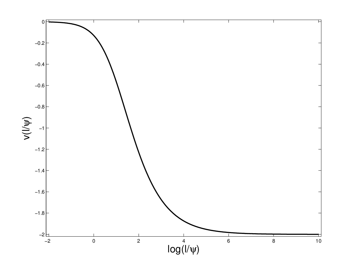
Figure 1: v⁡(l/ψCLOSEv(l/\psi) as a function of the dimensionless patch correlation length l/ψl/\psi. We consider the Gaussian approximation to the quasilocal correlation function. It is possible to check that vv approaches to the correct value given by the Eq.(41) for l/ψ≪1l/\psi\ll 1, and it approaches the predicted value v=−2v=-2 for larger arguments.

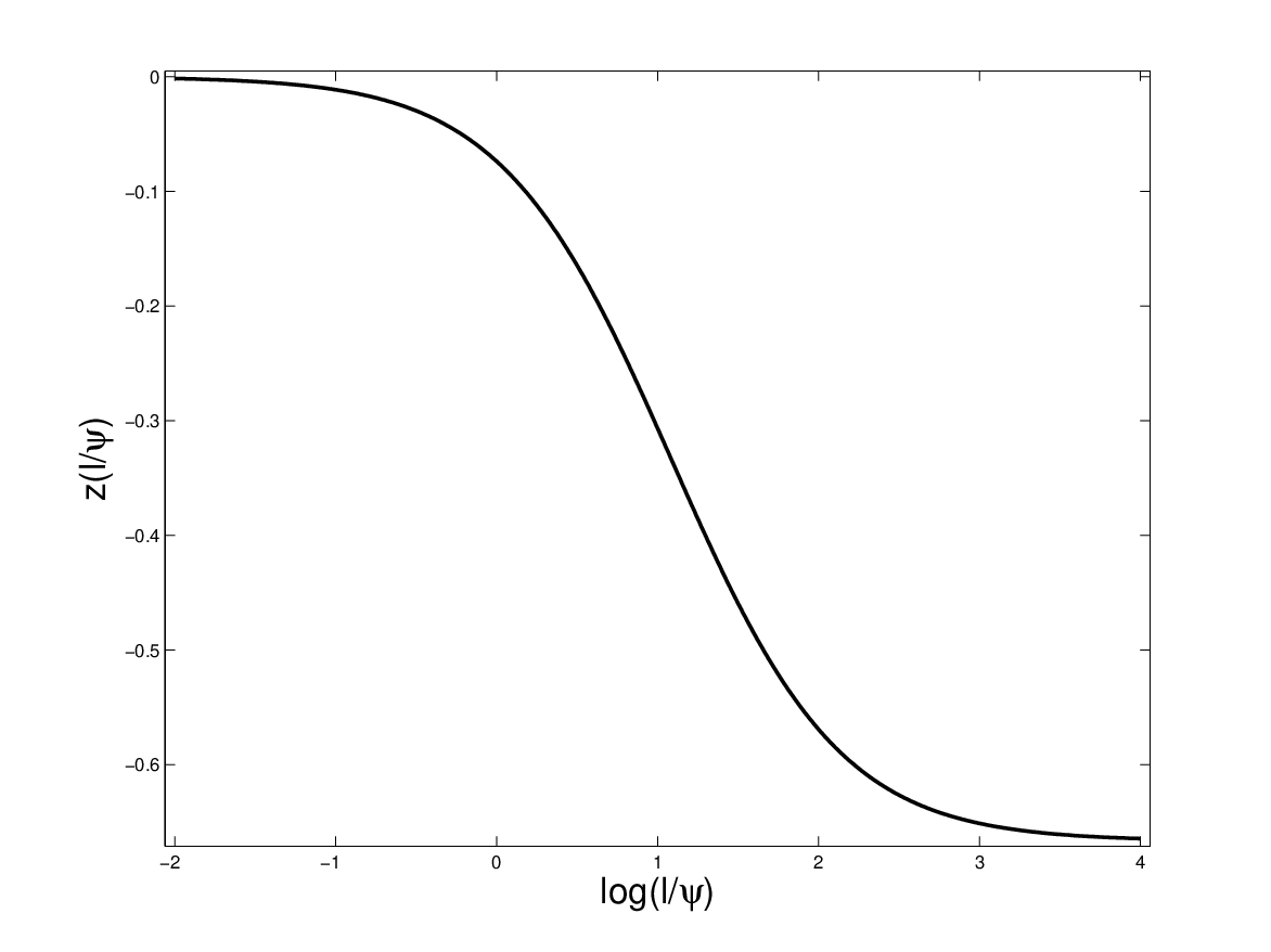
The functions vv and zz can be computed numerically; the results are shown in Figs.1 and 2. As expected, the numerical results have the correct behavior in the limits of small and large correlation lengths described in Eqs.(39) and (41) with g⁡(0)=π/4g(0)=\pi/4.

Refer to caption
Figure 2: z⁡(l/ψCLOSEz(l/\psi) as a function of the dimensionless patch correlation length l/ψl/\psi in the Gaussian model. It is possible to check that it approaches to the correct value given by the Eq.(41) for l/ψ≪1l/\psi\ll 1 and also to the predicted value z=−23z=-\frac{2}{3} when l≫ψl\gg\psi.

We also show the rate between the second and zeroth order contributions to the electrostatic energy, for the case of having a sphere in front of a plane. We consider a sphere of radius RR at a distance aa from a plane. Denoting by (rr,ϕ\phi) the polar coordinates in the (x1x_{1},x2x_{2}) plane the function ψ\psi reads

ψ⁡(r)=R⁡[aR+1−1−r2R2],\psi(r)=R\left[\frac{a}{R}+1-\sqrt{1-\frac{r^{2}}{R^{2}}}\right], (43)

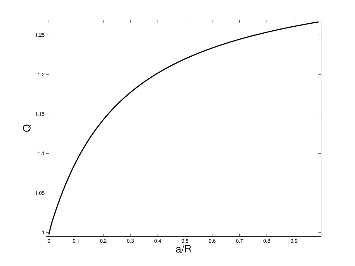
In the Fig. 3 we plot the ratio 𝒬=[UD​E(0)+UD​E(2)]UD​E(0){\cal Q}=\frac{\left[U^{(0)}_{DE}+U^{(2)}_{DE}\right]}{U^{(0)}_{DE}} as a function of ϵ=a/R\epsilon=a/R. As expected, there is a linear correction for small values of a/Ra/R. As the dependence with ℓ\ell is the same for UD​E(0)U^{(0)}_{DE} and UD​E(2)U^{(2)}_{DE} in the small patches limit ℓ≪a\ell\ll a (Eq.41), the value of 𝒬{\cal Q} does not depend on ℓ\ell for ℓ/R≪a/R\ell/R\ll a/R. We have checked this numerically.

Refer to caption
Figure 3: Rate 𝒬{\cal Q} as a function of a/Ra/R in the Gaussian approximation to the quasilocal patch correlation function, for l/R=0.001l/R=0.001. There is a lineal correction to the zeroth order.

IV.3 Correlation function with sharp-cutoffs

As a second example, we will consider the sharp-cutoff model proposed in Ref.[5]:

Ω~​(𝐤∥)=4​π​Vr​m​s2km​a​x2−km​i​n2​θ​(|𝐤∥|−km​i​n)​θ​(km​a​x−|𝐤∥|){\widetilde{\Omega}}({\mathbf{k}}_{\parallel})=\frac{4\pi V^{2}_{rms}}{k_{max}^{2}-k_{min}^{2}}\theta(|{\mathbf{k}}_{\parallel}|-k_{min})\theta(k_{max}-|{\mathbf{k}}_{\parallel}|) (44)

For this particular correlation, the functions VV and ZZ can be computed analytically

V⁡(ψ)\displaystyle V(\psi) =\displaystyle= −8​Vr​m​s2(km​a​x2−km​i​n2)​ψ3​[f0​(km​a​x​ψ)−f0​(km​i​n​ψ)]\displaystyle-\frac{8V^{2}_{rms}}{(k_{max}^{2}-k_{min}^{2})\psi^{3}}\left[f_{0}(k_{max}\psi)-f_{0}(k_{min}\psi)\right]
Z⁡(ψ)\displaystyle Z(\psi) =\displaystyle= Vr​m​s24​(km​a​x2−km​i​n2)​ψ3​[f2​(km​a​x​ψ)−f2​(km​i​n​ψ)],\displaystyle\frac{V^{2}_{rms}}{4(k_{max}^{2}-k_{min}^{2})\psi^{3}}\left[f_{2}(k_{max}\psi)-f_{2}(k_{min}\psi)\right]\,, (45)

where the functions f0f_{0} and f2f_{2} can be written in terms of polylogarithm functions L​in​(z)Li_{n}(z), and are given by

f0​(x)\displaystyle f_{0}(x) =\displaystyle= 12​x2​log⁡(1−e−2​x)−12​x​L​i2​(e−2​x)−14​L​i3​(e−2​x)\displaystyle\frac{1}{2}x^{2}\log(1-e^{-2x})-\frac{1}{2}x\,Li_{2}(e^{-2x})-\frac{1}{4}Li_{3}(e^{-2x})
f2​(x)\displaystyle f_{2}(x) =\displaystyle= 13​(−8​x3+8​x3​coth⁡(x)−4​x3​cosh⁡(x)sinh⁡(x)3+6​x4sinh⁡(x)4CLOSE\displaystyle\frac{1}{3}(-8x^{3}+8x^{3}\coth(x)-4x^{3}\frac{\cosh(x)}{\sinh(x)^{3}}+6\frac{x^{4}}{\sinh(x)^{4}} (46)
−\displaystyle- 24​x2​log⁡(1−e−2​x)+24​x​L​i2​(e−2​x)+12​L​i3​(e−2​x).\displaystyle 24x^{2}\log(1-e^{-2x})+24xLi_{2}(e^{-2x})+12Li_{3}(e^{-2x})\,.

These expressions contain as a particular case the constant potentials result, which can be obtained setting km​i​n=0k_{min}=0 and then taking the limit km​a​x=0k_{max}=0 (note that in this case the correlation function Ω~\widetilde{\Omega} becomes a δ\delta-function). Indeed, expanding f0f_{0} and f2f_{2} around x=0x=0 one can show that V⁡(ψ)V(\psi) and 3​Z​(ψ)3Z(\psi) tend to −2Vr​m​s2/ψ-2V_{rms}^{2}/\psi.

In the opposite limit, km​i​n=0k_{min}=0, km​a​x→∞k_{max}\to\infty we obtain

V≃−2​ζ​(3)​Vr​m​s2km​a​x2​ψ3Z≃−1+6​ζ​(3)6​Vr​m​s2km​a​x2​ψ3,V\simeq-2\zeta(3)\frac{V_{rms}^{2}}{k_{max}^{2}\psi^{3}}\quad Z\simeq-\frac{1+6\zeta(3)}{6}\frac{V_{rms}^{2}}{k_{max}^{2}\psi^{3}}\,, (47)

which, as expected, coincide with the short correlation limit given in Eq.(41).

An important feature of the sharp-cutoff model is that the electrostatic interaction energy between the surfaces is strongly suppressed when km​i​n≫1/ψk_{min}\gg 1/\psi. In this limit one can show that both VV and ZZ are proportional to exp⁡(−2​km​i​n​ψ)/ψ\exp(-2k_{min}\psi)/\psi.

V Conclusions

We have found explicit results for the leading and subleading terms in a DE approach to the calculation of the force due to patch potentials, for a family of experimentally relevant geometric configurations, in terms of the path potential correlation functions (which appear in our results inside simple integrals). Regarding those correlation functions, we have used specific models to obtain more explicit expressions for the coefficient functions the determine the DE to the interaction energy.

For the case of a gaussian correlation function, the DE of the interaction energy interpolates between (twice) the electrostatic result for a constant differential potential for large patches (ℓ≫ψ\ell\gg\psi)

UD​E=−ϵ0Vr​m​s2∫d2𝐱∥1ψ[1+13(∇ψ)2],U_{DE}=-\epsilon_{0}V_{rms}^{2}\int d^{2}{\mathbf{x}_{\parallel}}\,\frac{1}{\psi}\left[1+\frac{1}{3}(\nabla\psi)^{2}\right]\;, (48)

and a Casimir-like interaction energy for small patches (ℓ≪ψ\ell\ll\psi)

UD​E=−ϵ0​Vr​m​s2​ℓ2​ζ​(3)16∫d2𝐱∥1ψ3[1+0.569(∇ψ)2].U_{DE}=-\frac{\epsilon_{0}V_{rms}^{2}\ell^{2}\zeta(3)}{16}\int d^{2}{\mathbf{x}_{\parallel}}\,\frac{1}{\psi^{3}}\left[1+0.569(\nabla\psi)^{2}\right]\;. (49)

Similar results are valid for other correlation models, as the sharp-cutoff model, unless the correlation function Ω~​(𝐤∥){\widetilde{\Omega}}({\mathbf{k}}_{\parallel}) is strongly suppressed near the origin.

The results obtained in this paper may be useful in any experiment in which patch potentials could mask forces of different origin, by allowing for the identification of their contribution, not just their magnitude, but also their dependence on the geometry of the mirrors.

Acknowledgements

We would like to thank D. Dalvit and R. Decca for useful discussions that stimulated this research. C.D.F. thanks CONICET, ANPCyT and UNCuyo for financial support. The work of F.D.M. and F.C.L was supported by UBA, CONICET and ANPCyT.

Appendix A Expansion of GG in powers of η\eta

Let us present here a sketch of the approach we have used in order to expand GG in powers of η\eta. To that end we first recall that, in infinite unbounded space, an electrostatic potential φ⁡(𝐱)\varphi({\mathbf{x}}), which is solution to Poisson’s equation ∇2φ​(𝐱)=−ρ⁡(𝐱)\nabla^{2}\varphi({\mathbf{x}})=-\rho({\mathbf{x}}), must be a minimum of the functional

ℱ⁡[φ]=∫d3​𝐱​[12​(∇φ)2​(𝐱)−ρ⁡(𝐱)​φ​(𝐱)].{\mathcal{F}}[\varphi]\;=\;\int d^{3}{\mathbf{x}}\big[\frac{1}{2}(\nabla\varphi)^{2}({\mathbf{x}})-\rho({\mathbf{x}})\varphi({\mathbf{x}})\big]\;. (50)

Indeed, Poisson’s equation is tantamount here to the Euler-Lagrange equation corresponding to the extremal of the functional.

To consider an spatial region which is limited by the two surfaces LL and RR, where it satisfies Dirichlet boundary conditions, we may introduce two Lagrange multipliers λL\lambda_{L} and λR\lambda_{R}, and construct an augmented functional,

ℱ⁡[φ]\displaystyle{\mathcal{F}}[\varphi] =\displaystyle= ∫d3​𝐱​[12​(∇φ)2​(𝐱)−ρ⁡(𝐱)​φ​(𝐱)]\displaystyle\int d^{3}{\mathbf{x}}\big[\frac{1}{2}(\nabla\varphi)^{2}({\mathbf{x}})-\rho({\mathbf{x}})\varphi({\mathbf{x}})\big] (51)
+\displaystyle+ ∫d2​𝐱∥​[λL​(𝐱∥)​φ​(𝐱∥,0)+λR​(𝐱∥)​φ​(𝐱∥,ψ⁡(𝐱∥))].\displaystyle\int d^{2}{\mathbf{x}_{\parallel}}\left[\lambda_{L}({\mathbf{x}_{\parallel}})\,\varphi({\mathbf{x}_{\parallel}},0)+\lambda_{R}({\mathbf{x}_{\parallel}})\,\varphi({\mathbf{x}_{\parallel}},\psi({\mathbf{x}_{\parallel}}))\right]\;.

Thus, varying the field and the Lagrange multipliers independently, one finds the equation:

−∇2φ​(𝐱)−ρ⁡(𝐱)+λL​(𝐱∥)​δ​(x3)+λR​(𝐱∥)​δ​(x3−𝐱∥)= 0,-\nabla^{2}\varphi({\mathbf{x}})-\rho({\mathbf{x}})\,+\,\lambda_{L}({\mathbf{x}_{\parallel}})\,\delta(x_{3})+\lambda_{R}({\mathbf{x}_{\parallel}})\,\delta(x_{3}-{\mathbf{x}_{\parallel}})\;=\;0\;, (52)

plus

φ⁡(𝐱∥,0)=0,φ⁡(𝐱∥,ψ⁡(𝐱∥))=0.\varphi({\mathbf{x}_{\parallel}},0)=0\;\;,\;\;\;\;\varphi({\mathbf{x}_{\parallel}},\psi({\mathbf{x}_{\parallel}}))=0\;\;. (53)

We then recall that φ\varphi becomes the Dirichlet Green’s function: φ→G⁡(𝐱,𝐲)\varphi\to G({\mathbf{x}},{\mathbf{y}}) when ρ⁡(𝐱)→δ⁡(𝐱−𝐲)\rho({\mathbf{x}})\to\delta({\mathbf{x}}-{\mathbf{y}}). Naturally, Lagrange’s multipliers become also functions of the source point 𝐲{\mathbf{y}}.

Thus,

−∇𝐱2G​(𝐱,𝐲)=δ⁡(𝐱−𝐲)−λL​(𝐱∥,𝐲)​δ​(x3)−λR​(𝐱∥,𝐲)​δ​(x3−𝐱∥)= 0.-\nabla^{2}_{\mathbf{x}}G({\mathbf{x}},{\mathbf{y}})\;=\;\delta({\mathbf{x}}-{\mathbf{y}})\,-\,\lambda_{L}({\mathbf{x}_{\parallel}},{\mathbf{y}})\,\delta(x_{3})-\lambda_{R}({\mathbf{x}_{\parallel}},{\mathbf{y}})\,\delta(x_{3}-{\mathbf{x}_{\parallel}})\;=\;0\;. (54)

Acting with the inverse of the Laplacian on the previous equation, we see that:

G⁡(𝐱,𝐲)=G0​(𝐱,𝐲)−∫d2​𝐱∥′​[G0​(𝐱,𝐱∥′,0)​λL​(𝐱∥′,𝐲)+G0​(𝐱,𝐱∥′,ψ⁡(𝐱∥′))​λR​(𝐱∥′,𝐲)],G({\mathbf{x}},{\mathbf{y}})\;=\;G_{0}({\mathbf{x}},{\mathbf{y}})-\,\int d^{2}{\mathbf{x}^{\prime}_{\parallel}}\big[G_{0}({\mathbf{x}};{\mathbf{x}^{\prime}_{\parallel}},0)\lambda_{L}({\mathbf{x}^{\prime}_{\parallel}},{\mathbf{y}})+G_{0}({\mathbf{x}};{\mathbf{x}^{\prime}_{\parallel}},\psi({\mathbf{x}^{\prime}_{\parallel}}))\lambda_{R}({\mathbf{x}^{\prime}_{\parallel}},{\mathbf{y}})\big]\;, (55)

where G0G_{0} is the Green’s function in the absence of boundaries:

G0​(𝐱,𝐲)=∫d3​𝐤(2​π)3​ei​𝐤⋅(𝐱−𝐲)𝐤2.G_{0}({\mathbf{x}},{\mathbf{y}})\,=\,\int\frac{d^{3}{\mathbf{k}}}{(2\pi)^{3}}\frac{e^{i{\mathbf{k}}\cdot({\mathbf{x}}-{\mathbf{y}})}}{{\mathbf{k}}^{2}}\;. (56)

Evaluating (55) for points 𝐱{\mathbf{x}} belonging to either LL or RR, we obtain two equations which can be used to determine the Lagrange multipliers:

∫d2​𝐱∥′​[G0​(𝐱∥,0,𝐱∥′,0)​λL​(𝐱∥′,𝐲)+G0​(𝐱∥,0,𝐱∥′,ψ⁡(𝐱∥′))​λR​(𝐱∥′,𝐲)]=G0​(𝐱∥,0,𝐲)\int d^{2}{\mathbf{x}^{\prime}_{\parallel}}\big[G_{0}({\mathbf{x}_{\parallel}},0;{\mathbf{x}^{\prime}_{\parallel}},0)\lambda_{L}({\mathbf{x}^{\prime}_{\parallel}},{\mathbf{y}})+G_{0}({\mathbf{x}_{\parallel}},0;{\mathbf{x}^{\prime}_{\parallel}},\psi({\mathbf{x}^{\prime}_{\parallel}}))\lambda_{R}({\mathbf{x}^{\prime}_{\parallel}},{\mathbf{y}})\big]=G_{0}({\mathbf{x}_{\parallel}},0;{\mathbf{y}}) (57)

and

∫d2​𝐱∥′​[G0​(𝐱∥,ψ⁡(𝐱∥),𝐱∥′,0)​λL​(𝐱∥′,𝐲)+G0​(𝐱∥,ψ⁡(𝐱∥),𝐱∥′,ψ⁡(𝐱∥′))​λR​(𝐱∥′,𝐲)]\int d^{2}{\mathbf{x}^{\prime}_{\parallel}}\big[G_{0}({\mathbf{x}_{\parallel}},\psi({\mathbf{x}_{\parallel}});{\mathbf{x}^{\prime}_{\parallel}},0)\lambda_{L}({\mathbf{x}^{\prime}_{\parallel}},{\mathbf{y}})+G_{0}({\mathbf{x}_{\parallel}},\psi({\mathbf{x}_{\parallel}});{\mathbf{x}^{\prime}_{\parallel}},\psi({\mathbf{x}^{\prime}_{\parallel}}))\lambda_{R}({\mathbf{x}^{\prime}_{\parallel}},{\mathbf{y}})\big]
=G0​(𝐱∥,ψ⁡(𝐱∥),𝐲).=G_{0}({\mathbf{x}_{\parallel}},\psi({\mathbf{x}_{\parallel}});{\mathbf{y}})\;. (58)

Thus, introducing an index AA which may assume the values LL and RR, and two functions ζL=0\zeta_{L}=0, ζR​(𝐱∥)=ψ⁡(𝐱∥)\zeta_{R}({\mathbf{x}_{\parallel}})=\psi({\mathbf{x}_{\parallel}}), we may write the equations for the Lagrange multipliers as follows:

∫d2​𝐱∥′​𝕋A​B​(𝐱∥,𝐱∥′)​λB​(𝐱∥′,𝐲)=G0​(𝐱∥,ζA​(𝐱∥),𝐲).\int d^{2}{\mathbf{x}^{\prime}_{\parallel}}{\mathbb{T}}_{AB}({\mathbf{x}_{\parallel}},{\mathbf{x}^{\prime}_{\parallel}})\lambda_{B}({\mathbf{x}^{\prime}_{\parallel}},{\mathbf{y}})=G_{0}({\mathbf{x}_{\parallel}},\zeta_{A}({\mathbf{x}_{\parallel}});{\mathbf{y}})\;. (59)

where:

𝕋A​B​(𝐱∥,𝐱∥′)≡G0​(𝐱∥,ζA​(𝐱∥),𝐱∥′,ζB​(𝐱∥′)).{\mathbb{T}}_{AB}({\mathbf{x}_{\parallel}},{\mathbf{x}^{\prime}_{\parallel}})\equiv G_{0}({\mathbf{x}_{\parallel}},\zeta_{A}({\mathbf{x}_{\parallel}});{\mathbf{x}^{\prime}_{\parallel}},\zeta_{B}({\mathbf{x}^{\prime}_{\parallel}}))\;. (60)

Thus, the Green’s function, may be written as follows:

G⁡(𝐱,𝐲)\displaystyle G({\mathbf{x}},{\mathbf{y}}) =\displaystyle= G0​(𝐱,𝐲)\displaystyle G_{0}({\mathbf{x}},{\mathbf{y}}) (61)
−\displaystyle- ∫𝐱∥′,𝐱∥′′∑A,BG0​(𝐱,𝐱∥′,ζA​(𝐱∥′))​ΔA​B​(𝐱∥′,𝐱∥′′)​G0​(𝐱∥′′,ζB​(𝐱∥′′),𝐲)\displaystyle\int_{{\mathbf{x}^{\prime}_{\parallel}},{\mathbf{x}^{\prime\prime}_{\parallel}}}\sum_{A,B}\,G_{0}({\mathbf{x}};{\mathbf{x}^{\prime}_{\parallel}},\zeta_{A}({\mathbf{x}^{\prime}_{\parallel}}))\Delta_{AB}({\mathbf{x}^{\prime}_{\parallel}},{\mathbf{x}^{\prime\prime}_{\parallel}})G_{0}({\mathbf{x}^{\prime\prime}_{\parallel}},\zeta_{B}({\mathbf{x}^{\prime\prime}_{\parallel}});{\mathbf{y}})

where we introduced the inverse of 𝕋{\mathbb{T}}:

ΔA​B​(𝐱∥′,𝐱∥′′)=[𝕋−1]A​B​(𝐱∥′,𝐱∥′′).\Delta_{AB}({\mathbf{x}^{\prime}_{\parallel}},{\mathbf{x}^{\prime\prime}_{\parallel}})\;=\;\big[{\mathbb{T}}^{-1}\big]_{AB}({\mathbf{x}^{\prime}_{\parallel}},{\mathbf{x}^{\prime\prime}_{\parallel}})\;. (62)

Thus, the expansion for GG in powers of η\eta will be obtained by expanding Δ\Delta in powers of η\eta, which in turn requires to expand 𝕋{\mathbb{T}}. Note, however, that in the expressions for the different terms contributing to the energy, the Green’s function is evaluated at points that depend on ψ\psi, and that that function also appears in the normal derivatives. Thus, all of them have to be expanded in order to obtain the energy.

We conclude by writing the explicit form of the zeroth order term:

G(0)​(𝐱,𝐲)\displaystyle G^{(0)}({\mathbf{x}},{\mathbf{y}}) =\displaystyle= G0​(𝐱,𝐲)\displaystyle G_{0}({\mathbf{x}},{\mathbf{y}}) (63)
−\displaystyle- ∫𝐰∥,𝐳∥∑A,BG0​(𝐱,𝐰∥,ζA(0)​(𝐰∥))​ΔA​B(0)​(𝐰∥,𝐳∥)​G0​(𝐳∥,ζB(0)​(𝐳∥),𝐲)\displaystyle\int_{{\mathbf{w}_{\parallel}},{\mathbf{z}_{\parallel}}}\sum_{A,B}\,G_{0}({\mathbf{x}};{\mathbf{w}_{\parallel}},\zeta_{A}^{(0)}({\mathbf{w}_{\parallel}}))\Delta^{(0)}_{AB}({\mathbf{w}_{\parallel}},{\mathbf{z}_{\parallel}})G_{0}({\mathbf{z}_{\parallel}},\zeta^{(0)}_{B}({\mathbf{z}_{\parallel}});{\mathbf{y}})

where:

ΔA​B(0)​(𝐰∥,𝐳∥)=∫d2​𝐤∥(2​π)2​Δ~A​B(0)​(𝐤∥)​ei​𝐤∥⋅(𝐰∥−𝐳∥),\Delta^{(0)}_{AB}({\mathbf{w}_{\parallel}},{\mathbf{z}_{\parallel}})\;=\;\int\frac{d^{2}{\mathbf{k}_{\parallel}}}{(2\pi)^{2}}\;\widetilde{\Delta}^{(0)}_{AB}({\mathbf{k}_{\parallel}})e^{i{\mathbf{k}_{\parallel}}\cdot({\mathbf{w}_{\parallel}}-{\mathbf{z}_{\parallel}})}\;, (64)

with

[Δ~(0)]​(𝐤∥)=2​|𝐤∥|1−e−2​|𝐤∥|​a​(1−e−|𝐤∥|​a−e−|𝐤∥|​a1)[\widetilde{\Delta}^{(0)}]({\mathbf{k}_{\parallel}})\,=\,\frac{2|{\mathbf{k}_{\parallel}}|}{1-e^{-2|{\mathbf{k}_{\parallel}}|a}}\left(\begin{array}[]{cc}1&-e^{-|{\mathbf{k}_{\parallel}}|a}\\ -e^{-|{\mathbf{k}_{\parallel}}|a}&1\end{array}\right) (65)

References

  • [1] P. W. Milonni, The Quantum Vacuum, Academic Press, San Diego, 1994; M. Bordag, U. Mohideen, and V. M. Mostepanenko, Phys. Rep. 353, 1 (2001); K. A. Milton, The Casimir Effect: Physical Manifestations of the Zero-Point Energy (World Scientific, Singapore, 2001); K. A. Milton, J. Phys. A: Math. Gen. 37, R209 (2004); S.K. Lamoreaux, Rep. Prog. Phys. 68, 201 (2005); M. Bordag, G.L. Klimchitskaya, U. Mohideen, and V. M. Mostepanenko, Advances in the Casimir Effect, Oxford University Press, Oxford, 2009.
  • [2] R. Smoluchowski, Phys. 60, 661 (1941); N. D. Lang and W. Kohn, Phys. Rev. B3, 1215 (1971); N. Gaillard et. al., Appl. Phys. Lett. 89, 154101 (2006).
  • [3] See for instance S.E. Pollack, S. Schlamminger and J.H. Gundlach, Phys. Rev. Lett. 101, 071101 (2008); L. Deslauriers, et al, Phys. Rev. Lett.97,103007 (2006); J.D. Carter and J.D.D. Martin, Phys. Rev. A 83, 032902 (2011).
  • [4] R. O. Behunin, D. A. R. Dalvit, R. S. Decca and C. C. Speake, arXiv:1304.4074 [gr-qc].
  • [5] C. C. Speake and C. Trenkel, Phys. Rev. Lett. 90, 160403 (2003).
  • [6] R. O. Behunin, F. Intravaia, D. A. R. Dalvit, P. A. Maia Neto and S. Reynaud, Phys. Rev. A 85, 012504 (2012).
  • [7] B. V. Derjaguin and I. I. Abrikosova, Sov. Phys. JETP 3, 819 (1957) ; B. V. Derjaguin, Sci. Am. 203, 47 (1960); J. Blocki, J. Randrup, W. J. Swiatecki, and C. F. Tsang, Ann. Phys. NY 105, 427 (1977).
  • [8] R. O. Behunin, Y. Zeng, D. A. R. Dalvit and S. Reynaud, Phys. Rev. A 86, 052509 (2012).
  • [9] C. D. Fosco, F. C. Lombardo and F. D. Mazzitelli, Phys. Rev. D 84, 105031 (2011); C. D. Fosco, F. C. Lombardo and F. D. Mazzitelli, Phys. Rev. D 85, 125037 (2012); C. D. Fosco, F. C. Lombardo and F. D. Mazzitelli, Phys. Rev. D 86, 045021 (2012); G. Bimonte, T. Emig, R. L. Jaffe, M. Kardar, Europhys. Lett. 97, 50001 (2012).
  • [10] C. D. Fosco, F. C. Lombardo and F. D. Mazzitelli, Annals Phys. 327, 2050 (2012).
  • [11] C. D. Fosco, F. C. Lombardo and F. D. Mazzitelli, Phys. Rev. D 86, 125018 (2012).