Single soft gluon emission at two loops
Abstract
We study the single soft-gluon current at two loops with two energetic partons in massless perturbative QCD, which describes, for example, the soft limit of the two-loop amplitude for . The results are presented as Laurent expansions in in spacetime dimension. We calculate the expansion to order analytically, which is a necessary ingredient for Higgs production at hadron colliders at next-to-next-to-next-to-leading order in the soft-virtual approximation. We also give two-loop results of the single soft-gluon current in Super-Yang-Mills theory, and find that it has uniform transcendentality. By iteration relation of splitting amplitudes, our calculations can determine the three-loop single soft-gluon current to order in Super-Yang-Mills theory in the limit of large .
I Introduction
Amplitudes in gauge theory develop infrared divergences when one or multiple external partons become soft/collinear. Fortunately, in the soft/collinear limit, there exist universal factorization properties for such amplitudes, which are the foundation of higher-order perturbative-QCD computations. Extensive discussion on the factorization of gauge-theory amplitudes in the infrared region can be found, for example, in Refs. [1, 2, 3, 4, 5, 6, 7, 8, 9, 10, 11, 12, 13, 14, 15, 16, 17, 18, 19, 20, 21, 22, 23, 24].
In QCD, the radiation of an arbitrary number of soft gluons off a tree-level amplitude can be obtained using the well-known Berends-Giele recursion relation [3]. Due to the long-range properties of soft gluon radiation, amplitudes in the soft limit have non-local color correlations. Compact expressions for tree-level amplitudes with two soft partons have been obtained in the color space formalism in Ref. [7]. Emission of a single soft gluon from a generic one-loop amplitude have also been studied by several groups [8, 12, 14, 15]. These results have been proven to be important in the program of next-to-next-to-leading order (NNLO) QCD computations for jet physics, see for example Refs. [25, 26, 27, 28, 29, 30, 31].
While the NNLO revolution is under way, there is strong motivation for going one order in further. This is driven by both experimental and theoretical demands. On the experimental side, the discovery of Higgs boson marks one of the most important progress in particle physics in the last few decades [32, 33]. It’s certainly important to give the most precise theoretical prediction for its production cross section. On the theory side, uncertainties estimated by scale variation for Higgs production is around at NNLO [34, 35, 36, 37], and improved to by including soft-gluon resummation up to next-to-next-to-leading logarithmic accuracy [38]. Further decreasing the scale uncertainties to percent level requires the computation of next-to-next-to-next-to-leading order (NNNLO) QCD corrections.
In this paper we consider single soft-gluon radiation at two loops, which plays an important role in NNNLO QCD corrections, similar to the one-loop soft-gluon current does in NNLO computations, see for example, Refs. [25, 26, 27, 39]. To simplify the situation, we confine ourselves to the case that only two hard partons are present. This corresponds to the cases such as dijet, deep-inelastic scattering, or Drell-Yan/Higgs production at hadron collider. Previously, such amplitudes have been derived [19] by taking the soft limit of collinear splitting amplitudes at two loops to order , using the two-loop aamplitudes for [40, 41] and [42]. However, for a NNNLO computation, one needs the Laurent expansion in through the terms, which we have given for the first time in this paper. Our results for the two-loop soft amplitude agree with the soft limit of the two-loop splitting amplitudes [18, 19] through the terms, serving as a strong check of our calculation.
As a by-product, we obtain the soft-gluon current in Super-Yang-Mills theory to order , which coincides with the QCD result at leading transcendentality. We also derive the soft limit of splitting amplitudes at three loops through order at leading order of , using the results of Refs. [43, 44].
The paper is organized as follows. In Sec. II, we review the general result on the factorization of the single soft-gluon current at tree level and one loop. In Sec. III we calculate the soft-gluon current to two loops. We conclude at Sec. IV. We present some details for the computation of one of the master integral in the appendix.
II Review of the soft-gluon current
In this section we review the factorization of amplitudes in the soft limit, closely following the notation in Ref. [15]. It’s well-known [2, 4] that tree-level QCD amplitudes with two hard partons and one soft gluon can be written as
| (1) |
where , and is the tree-level amplitude for hard partons (massless quark or gluon) and one soft gluon, and is the corresponding amplitude with the soft gluon stripped off. Dependence of the amplitudes on the extra colorless particles in the process is left implicit. The symbol means that we have neglected terms that are less singular than . is the strong coupling constant, is the mass scale introduced by continuing the space-time dimension to dimension. is the quadratic Casimir invariant. if parton is a gluon, if parton is a quark, where and , with being the number of color. Note that the functional dependence of the eikonal function is uniquely determined by its invariance under the rescaling of and , which is a simple consquence of the QCD Feynman rule in the eikonal limit. In our convention, all momenta are massless and have positive-definite energies. The generalization of Eq. (1) to processes with any number of hard partons can be found, for example, in Ref. [7].
At the one-loop level, Eq. (1) receives quantum corrections, which can be written as
| (2) | |||||
where denotes complex conjugate. is the th order in unrenormalized amplitudes in dimensional regularization, where UV and IR divergences are simutaneously regularized by the dimensional regularization parameter . The one-loop corrections to the eikonal function have been calculated to be [8, 12, 14, 15]
| (3) |
where
| (4) |
and if both and are incoming, otherwise . Note that the one-loop eikonal function doesn’t depend on , which may be explained by the non-abelian exponentiation theorem [45, 46], if one replaces the polarization summation for the soft gluon by a cut propagator. Eq. (3), and its generalization to processes with any number of hard partons have been used, for example, in the calculation of soft-virtual approximation to Higgs production at NNLO [47, 48, 49], in the calculation of the two-loop soft function in soft-collinear-effective theory [50, 51, 52, 53], and in the construction of subtraction term in general NNLO corrections [25, 26, 27, 39].
III Calculation of the two-loop soft-gluon current
At two loops, the factorized soft-gluon current has the form
| (5) | |||||
The two-loop generalization is consistent with the soft limit of two-loop collinear splitting amplitudes [18, 19]. For the latter, it has been shown that similar factorization form holds to all orders in [9]. The two-loop eikonal function, , is known through the order terms by taking the soft limit of the two-loop collinear splitting amplitudes [18, 19] or the two-loop squared amplitudes for and [40, 41, 42]. However, for computation accurate to NNNLO, one also needs the order and order terms. In this section, we calculate the Laurent expansions of in through order , using a method different from Refs. [19].
In Ref. [15], the one-loop soft-gluon current is derived by taking the eikonal approximation of the integrand of the amplitudes before the loop integrals are carried out. This has the advantage that the one-loop eikonal function can be directly obtained without the subtraction of the product of the tree-level eikonal function and the one-loop squared amplitude, that is, the second line of Eq. (2). The same procedure can be used in the calculation of the two-loop eikonal function.
Specifically, we generate the integrand corresponding to the interference of tree-level and two-loop amplitudes, the first line of Eq. (5). For this purpose, we consider the process , keeping in mind that the eikonal function is independent of the colorless particles in the process. Summation of polarization for the external gluon is done in Feynman gauge. We then take the eikonal approximation of the integrand, assumming that the energy of the internal and external gluons are parametrically smaller then and . The integrand after the eikonal approximation is taken can also be generated by treating and as two out-going Wilson lines, whose directions are given by and . We have checked that this indeed gives the same integrand 11 1 We use QGRAF [54] extensively in generating various diagrams.. We note that after the eikonal approximation is taken on the right hand side of Eq. (5), the second and the third lines of it vanish. The reason is that and become scaleless integrals and vanish identically in dimensional regularization. Therefore, The two-loop eikonal function can be obtained by evaluating the resulting integrand, without the need of subtraction.
III.1 Warm up: one-loop soft-gluon current
For the convenience of reader, we reproduce the one-loop results in this section. At one loop, there is only one non-zero diagram (from now on eikonal approximation is assumed for the integrand), which is depicted in Fig. 1. All the remaining diagrams are zero in dimensional regularization, because their loop integrals are scaleless. One example of such a vanishing diagram is depicted in Fig. 2. We note that the external soft-gluon momentum only enters the loop integral through . However, the invariance of the integral under the rescaling of and demands that a factor of must be generated per loop. This is impossible for this diagram, leading to the conclusion that it must vanish.


We calculate the interference between the one-loop non-zero diagram, Fig. 1, and the tree-level diagrams in Fig. 3. The one-loop eikonal function can then be extracted from the one-loop integral in the interference term, which, after some simplification, reads
| (6) |
where the Feynman prescription is implicitly understood for all propagators in square brackets, for example, . Carrying out the loop integral, we reproduce the one-loop eikonal function in Eq. (3).
III.2 Two-loop soft-gluon current
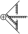
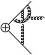
As explained above, the two-loop eikonal function can be extracted from the calculation of the non-vanishing diagrams at two-loop level, as depicted in Fig. 4. The grey blobs represent all possible two-point and three point insertions, where no eikonal approximation is made. We include flavour of massless fermions and flavour of massless scalar in the blob, besides the gluon. In QCD, , . Before describing the calculation of these diagrams, we comment on the diagrams that vanish identically. There are two classes of vanishing diagrams. The first class vanishes due to color or Lorentz algebra. An example of it is depicted in Fig. 5a. The second class vanishes because the corresponding loop integral is scaleless, as in Fig. 5b. Because of the vanishing of these two classes of diagrams, the actual number of diagrams that need to be evaluated is significantly reduced.
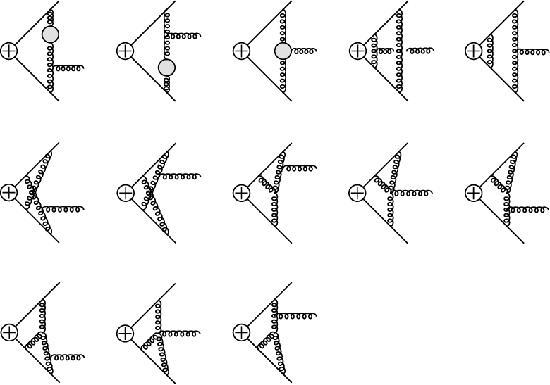


We now come to the actual evaluation of the non-zero diagrams in Fig. 4. We calculate the interference terms between the tree-level diagrams in Fig. 3 and the two-loop diagrams in Fig. 4. After the evaluation of color factor and kinematical factor, the resulting loop integrals are reduced to three master integrals in Fig. 6. To that end, we use the techniques of Integration-By-Parts (IBP) [55, 56], implemented in the MATHEMATICA package FIRE [57] using the Laporta algorithm [58]. The reduction to master integrals has also been cross checked using a different MATHEMATICA package LiteRed [59]. The results after the IBP reduction procedure can be written as
| (7) | |||||
The parameter selects the particular variant of dimensional regularization. For the scheme is the conventional dimensional regularization scheme, while for it is the four-dimensional helicity scheme (FDH) [60, 61].
There are three master integrals encountered in this computation. They are defined as
| (8) |
where dependences in the propagators are understood. The first two masters are calculated to all orders in . For the last master integral, we give the Laurent expansion of it to order , which is the order relevant for NNNLO computation. The details of the computation of the last integral are presented in the appendix. Here we only list the results for the three master integrals:
| (9) | |||||
where is the Riemann zeta vaule, . It’s interesting to note that coincides with the soft limit of the corresponding master integral in full QCD, where no eikonal approximation is taken in the denominator. The latter was calculated in Ref. [62] to order . This is probably due to the fact that the divergences in have only infrared origin. While we have only presented the Laurent expansions of to order analytically, the higher-order terms can easily be obtained numerically, using its two-fold Mellin-Barnes integral representation derived in the appendix, and the MBintegrate routine of Czakon [63]. For example, the next three terms in the expansion of are given by
| (10) |
However, it’s difficult to convert them into Riemann zeta values due to lack of significant digits.
Substituting the master integral into Eq. (7) and setting , we obtain the two-loop eikonal function in QCD in the conventional dimensional regularization scheme (),
| (11) | |||||
Eq. (11) is the main result of this paper. We remind the reader that this result is for the unrenormalized amplitudes. To obtain the renormalized ones, one only needs to perform a renormalization on the strong coupling . We have checked Eq. (11) against the two-loop splitting amplitudes in the soft limit calculated in Refs. [18, 19], and found full agreement to order . To the best of our knowledge, the order and terms presented in this paper are new.
III.3 Single soft-gluon current in Super-Yang-Mills theory
Using the generic results presented above, it’s straightforward to obtain the single soft-gluon current in Super-Yang-Mills theory, by setting , , and (corresponding to FDH scheme [60, 61]) in Eq. (7):
| (12) |
This result is remarkably simple. It becomes obvious that the result in Super-Yang-Mills theory has uniform transcendentality, as long as does. Substituting the explicit form of the master integrals into Eq. (12), we obtain
| (13) |
We note that at leading transcendentality, the eikonal soft function in Super-Yang-Mills theory coincides with the one in QCD through , as also happens in some other context [64].
It’s also interesting to notice that Eq. (13) can be reorganized as [65] 22 2 We are grateful to Lance Dixon for pointing us to the discussion in the rest of this section.
| (14) | |||||
where is the soft limit of the one-loop collinear splitting amplitudes in Super-Yang-Mills theory (up to an overall -dependent factor, same below), and [65]. Eq. (14) makes explicit the iterative structure of splitting amplitudes and eikonal function [43]. Eq. (14) also determines the soft limit of two-loop splitting amplitudes beyond order ,
| (15) | |||||
At three loops, the soft limit of splitting amplitudes at leading color is predicted to be [43]
| (16) |
where has been calculated through order [44],
| (17) |
with . Using the above results, we obtain
| (18) |
For completeness, the eikonal function at leading color is then given by
| (19) |
We note that Eq. (18) is actually exact through order for finite . There are potential corrections, starting from order . Unlike the one-loop and two-loop cases, these corrections would depend explicitly on the color representation of the hard partons, through the product of fourth order invariant tensor, . An explicit calculation of these corrections would be necessary in obtaining them.
IV Conclusion
In this paper we have computed the single soft-gluon current to two-loop order. we have compared our results with those in Refs. [18, 19], and found full agreement to order . The order and order terms presented in this paper are new. As a by-product, we have also given the soft-gluon current in Super-Yang-Mills theory to order , which in turn enables us to derive the splitting amplitudes in the soft limit, or the single soft-gluon current, at three loops and large , using the results of Refs. [43, 44]. We observe uniform transcendentality for the single soft-gluon current in Super-Yang-Mills theory, and confirm that the leading transcendentality terms for the eikonal function are the same in QCD and Super-Yang-Mills theory at two loops, up to order .
The main purpose of the computation done in this paper is to provide the necessary ingredient for a calculation of Higgs production cross section at hadron collider at NNNLO. A lot of progress have been made recently in this direction [67, 68, 69, 70, 71, 72]. A useful step towards the full NNNLO QCD corrections is the soft-virtual approximation at NNNLO. Using the results presented in this paper, the cross section for Higgs one gluon emission can be computed by trivially integrating over the soft-gluon phase space. The cross section for Higgs 3 partons production in the soft limit has also been calculated recently in an impressive paper [70]. The only missing piece is the cross section for Higgs 2 partons production at one loop in the soft limit. It’s reasonable to expect that the soft-virtual approximation for Higgs production at hadron collider at NNNLO will be available in the foreseeable future.
Besides Higgs physics, the soft gluon current at two loops is also useful in soft-collinear-effective theory [50, 51, 52, 53]. For example, the two-loop soft gluon current can be used to calculate soft function at NNNLO. Finally, we have only computed this soft gluon current with two energetic partons, or two Wilson lines. It’s certainly interesting to extend our results to processes with an arbitrary number of Wilson lines. This will be relevant to jet physics at NNNLO. It will also be useful in understanding the structure of infrared divergences for multiple Wilson lines at three loops, see for example, Ref. [73].
Acknowledgements.
We are grateful to Lance Dixon for careful reading of the manuscript and invaluable suggestions. We also thank Michael Peskin for useful discussion. This research is supported by the US Department of Energy under contract DE–AC02–76SF00515. HXZ would like to thank Kavli Institute for Theoretical Physics at UC Santa Barbara and the Erwin Schrödinger Institute at University of Vienna for hospitality while part of this work was carried out. While this paper was being completed, we learned of independent work [74] by Claude Duhr and Thomas Gehrmann obtaining the soft-gluon current to all orders in , which is in full agreement with the Laurent expansions of the soft-gluon current to order derived in this paper.*
Appendix A Evaluation of the master integral to order
In this appendix, we briefly explain the evaluation of the most difficult master integral, . In fact, and can be obtained by deleting two propagators from . We proceed by first performing the sub-loop integral by Feynman’s trick,
| (20) | |||||
where
| (21) |
The resulting Feynman parameter integral over can be factorized by introducing a two-fold Mellin-Barnes integral,
| (22) | |||||
where the contour for separates the poles of from those of . After this step, the Feynman parameter integral over can be done in closed form in terms of functions. The remaining sub-loop integral has the form
| (23) |
which can be straightforwardly done. We then arrive at a two-fold Mellins-Barnes integral representation for ,
| (24) | |||||
We were not able to find an all order in solution of this integral. Instead, we calculate the Laurent expansion of the Mellin-Barnes integral to order , which is relevant for NNNLO phenomenology. To that end, we make use of the MATHEMATICA pachages MB [63] and BARNESROUTINES of D. Kosower to resolve the singularity, to expand the integrand in , and to apply the Barnes lemma in an automatic way, which results in a series of one-fold and two-fold Mellin-Barnes integrals. The one-fold integral can easily be done numerically using MATHEMATICA’s NIntegrate routine, and the results can be converted into Riemann zeta values using the PSLQ algorithm [75, 76]. The only remaining two-fold Mellin-Barnes integral is
| (25) |
where is the logarithmic derivative of function, and the integration contours are straight vertical lines defined by
| (26) |
The integral can be performed by closing the contour to the left or right, and summing up the residues at the poles. The results are double sums of the form
| (27) |
where are nested harmonic sums defined in Ref. [77]. The summation can be conveniently done using XSummer [78]. The final result for this master integral is checked numerically using the package FIESTA [79] and the author’s personal tool, based on the method of sector decomposition [80].
References
- [1] G. Altarelli and G. Parisi, Nucl.Phys. B126, 298 (1977).
- [2] A. Bassetto, M. Ciafaloni, and G. Marchesini, Phys.Rept. 100, 201 (1983).
- [3] F. A. Berends and W. Giele, Nucl.Phys. B313, 595 (1989).
- [4] Y. L. Dokshitzer, V. A. Khoze, A. H. Mueller, and S. Troian, Basics of perturbative QCD, Editions Frontières, Gif-sur-Yvette (1991).
- [5] R. K. Ellis, W. J. Stirling, and B. Webber, QCD and Collider Physics, Cambridge University Press, Cambridge (1996).
- [6] J. M. Campbell and E. W. N. Glover, Nucl.Phys. B527, 264 (1998), arXiv:hep-ph/9710255 [hep-ph] .
- [7] S. Catani and M. Grazzini, Nucl.Phys. B570, 287 (2000a), arXiv:hep-ph/9908523 [hep-ph] .
- [8] Z. Bern and G. Chalmers, Nucl.Phys. B447, 465 (1995), arXiv:hep-ph/9503236 [hep-ph] .
- [9] D. A. Kosower, Nucl.Phys. B552, 319 (1999), arXiv:hep-ph/9901201 [hep-ph] .
- [10] S. Catani and M. Grazzini, Phys.Lett. B446, 143 (1999), arXiv:hep-ph/9810389 [hep-ph] .
- [11] V. Del Duca, A. Frizzo, and F. Maltoni, Nucl.Phys. B568, 211 (2000), arXiv:hep-ph/9909464 [hep-ph] .
- [12] Z. Bern, V. Del Duca, and C. R. Schmidt, Phys.Lett. B445, 168 (1998), arXiv:hep-ph/9810409 [hep-ph] .
- [13] S. Catani, Phys.Lett. B427, 161 (1998), arXiv:hep-ph/9802439 [hep-ph] .
- [14] Z. Bern, V. Del Duca, W. B. Kilgore, and C. R. Schmidt, Phys.Rev. D60, 116001 (1999), arXiv:hep-ph/9903516 [hep-ph] .
- [15] S. Catani and M. Grazzini, Nucl.Phys. B591, 435 (2000b), arXiv:hep-ph/0007142 [hep-ph] .
- [16] D. A. Kosower, Phys.Rev.Lett. 91, 061602 (2003), arXiv:hep-ph/0301069 [hep-ph] .
- [17] S. Catani, D. de Florian, and G. Rodrigo, Phys.Lett. B586, 323 (2004), arXiv:hep-ph/0312067 [hep-ph] .
- [18] Z. Bern, L. J. Dixon, and D. A. Kosower, JHEP 0408, 012 (2004), arXiv:hep-ph/0404293 [hep-ph] .
- [19] S. Badger and E. W. N. Glover, JHEP 0407, 040 (2004), arXiv:hep-ph/0405236 [hep-ph] .
- [20] A. Gehrmann-De Ridder, T. Gehrmann, E. W. N. Glover, and G. Heinrich, JHEP 0711, 058 (2007), arXiv:0710.0346 [hep-ph] .
- [21] I. Bierenbaum, M. Czakon, and A. Mitov, Nucl.Phys. B856, 228 (2012), arXiv:1107.4384 [hep-ph] .
- [22] S. Catani, D. de Florian, and G. Rodrigo, JHEP 1207, 026 (2012), arXiv:1112.4405 [hep-ph] .
- [23] J. Currie, E. W. N. Glover, and S. Wells, JHEP 1304, 066 (2013), arXiv:1301.4693 [hep-ph] .
- [24] I. Feige and M. D. Schwartz, (2013), arXiv:1306.6341 [hep-th] .
- [25] A. Gehrmann-De Ridder, T. Gehrmann, and E. W. N. Glover, JHEP 0509, 056 (2005), arXiv:hep-ph/0505111 [hep-ph] .
- [26] G. Somogyi, Z. Trocsanyi, and V. Del Duca, JHEP 0506, 024 (2005), arXiv:hep-ph/0502226 [hep-ph] .
- [27] M. Czakon, Phys.Lett. B693, 259 (2010), arXiv:1005.0274 [hep-ph] .
- [28] P. Baernreuther, M. Czakon, and A. Mitov, Phys.Rev.Lett. 109, 132001 (2012), arXiv:1204.5201 [hep-ph] .
- [29] M. Czakon, P. Fiedler, and A. Mitov, Phys.Rev.Lett. 110, 252004 (2013), arXiv:1303.6254 [hep-ph] .
- [30] A. G.-D. Ridder, T. Gehrmann, E. W. N. Glover, and J. Pires, Phys.Rev.Lett. 110, 162003 (2013), arXiv:1301.7310 [hep-ph] .
- [31] R. Boughezal, F. Caola, K. Melnikov, F. Petriello, and M. Schulze, JHEP 1306, 072 (2013), arXiv:1302.6216 [hep-ph] .
- [32] G. Aad et al. (ATLAS Collaboration), Phys.Lett. B716, 1 (2012), arXiv:1207.7214 [hep-ex] .
- [33] S. Chatrchyan et al. (CMS Collaboration), Phys.Lett. B716, 30 (2012), arXiv:1207.7235 [hep-ex] .
- [34] R. V. Harlander and W. B. Kilgore, Phys.Rev.Lett. 88, 201801 (2002), arXiv:hep-ph/0201206 [hep-ph] .
- [35] C. Anastasiou and K. Melnikov, Nucl.Phys. B646, 220 (2002), arXiv:hep-ph/0207004 [hep-ph] .
- [36] V. Ravindran, J. Smith, and W. L. van Neerven, Nucl.Phys. B665, 325 (2003), arXiv:hep-ph/0302135 [hep-ph] .
- [37] S. Catani and M. Grazzini, Phys.Rev.Lett. 98, 222002 (2007), arXiv:hep-ph/0703012 [hep-ph] .
- [38] S. Dittmaier et al. (LHC Higgs Cross Section Working Group), (2011), arXiv:1101.0593 [hep-ph] .
- [39] R. Boughezal, K. Melnikov, and F. Petriello, Phys.Rev. D85, 034025 (2012), arXiv:1111.7041 [hep-ph] .
- [40] L. Garland, T. Gehrmann, E. N. Glover, A. Koukoutsakis, and E. Remiddi, Nucl.Phys. B627, 107 (2002a), arXiv:hep-ph/0112081 [hep-ph] .
- [41] L. Garland, T. Gehrmann, E. W. N. Glover, A. Koukoutsakis, and E. Remiddi, Nucl.Phys. B642, 227 (2002b), arXiv:hep-ph/0206067 [hep-ph] .
- [42] T. Gehrmann, M. Jaquier, E. Glover, and A. Koukoutsakis, JHEP 1202, 056 (2012), arXiv:1112.3554 [hep-ph] .
- [43] Z. Bern, L. J. Dixon, and V. A. Smirnov, Phys.Rev. D72, 085001 (2005), arXiv:hep-th/0505205 [hep-th] .
- [44] M. Spradlin, A. Volovich, and C. Wen, Phys.Rev. D78, 085025 (2008), arXiv:0808.1054 [hep-th] .
- [45] J. Gatheral, Phys.Lett. B133, 90 (1983).
- [46] J. Frenkel and J. Taylor, Nucl.Phys. B246, 231 (1984).
- [47] S. Catani, D. de Florian, and M. Grazzini, JHEP 0105, 025 (2001), arXiv:hep-ph/0102227 [hep-ph] .
- [48] R. V. Harlander and W. B. Kilgore, Phys.Rev. D64, 013015 (2001), arXiv:hep-ph/0102241 [hep-ph] .
- [49] D. de Florian and J. Mazzitelli, JHEP 1212, 088 (2012), arXiv:1209.0673 [hep-ph] .
- [50] C. W. Bauer, S. Fleming, and M. E. Luke, Phys.Rev. D63, 014006 (2000), arXiv:hep-ph/0005275 [hep-ph] .
- [51] C. W. Bauer, S. Fleming, D. Pirjol, and I. W. Stewart, Phys.Rev. D63, 114020 (2001), arXiv:hep-ph/0011336 [hep-ph] .
- [52] C. W. Bauer, D. Pirjol, and I. W. Stewart, Phys.Rev. D65, 054022 (2002), arXiv:hep-ph/0109045 [hep-ph] .
- [53] M. Beneke, A. Chapovsky, M. Diehl, and T. Feldmann, Nucl.Phys. B643, 431 (2002), arXiv:hep-ph/0206152 [hep-ph] .
- [54] P. Nogueira, J.Comput.Phys. 105, 279 (1993).
- [55] K. Chetyrkin and F. Tkachov, Nucl.Phys. B192, 159 (1981).
- [56] F. Tkachov, Phys.Lett. B100, 65 (1981).
- [57] A. Smirnov, JHEP 0810, 107 (2008), arXiv:0807.3243 [hep-ph] .
- [58] S. Laporta, Int.J.Mod.Phys. A15, 5087 (2000), arXiv:hep-ph/0102033 [hep-ph] .
- [59] R. Lee, (2012), arXiv:1212.2685 [hep-ph] .
- [60] Z. Bern and D. A. Kosower, Nucl.Phys. B379, 451 (1992).
- [61] Z. Bern, A. De Freitas, L. J. Dixon, and H. Wong, Phys.Rev. D66, 085002 (2002), arXiv:hep-ph/0202271 [hep-ph] .
- [62] T. Gehrmann and E. Remiddi, Nucl.Phys. B601, 248 (2001), arXiv:hep-ph/0008287 [hep-ph] .
- [63] M. Czakon, Comput.Phys.Commun. 175, 559 (2006), arXiv:hep-ph/0511200 [hep-ph] .
- [64] A. Kotikov, L. Lipatov, A. Onishchenko, and V. Velizhanin, Phys.Lett. B595, 521 (2004), arXiv:hep-th/0404092 [hep-th] .
- [65] C. Anastasiou, Z. Bern, L. J. Dixon, and D. Kosower, Phys.Rev.Lett. 91, 251602 (2003), arXiv:hep-th/0309040 [hep-th] .
- [66] Z. Bern, M. Czakon, L. J. Dixon, D. A. Kosower, and V. A. Smirnov, Phys.Rev. D75, 085010 (2007), arXiv:hep-th/0610248 [hep-th] .
- [67] A. Pak, M. Rogal, and M. Steinhauser, JHEP 1109, 088 (2011), arXiv:1107.3391 [hep-ph] .
- [68] C. Anastasiou, S. Buehler, C. Duhr, and F. Herzog, JHEP 1211, 062 (2012), arXiv:1208.3130 [hep-ph] .
- [69] M. Höschele, J. Hoff, A. Pak, M. Steinhauser, and T. Ueda, Phys.Lett. B721, 244 (2013), arXiv:1211.6559 [hep-ph] .
- [70] C. Anastasiou, C. Duhr, F. Dulat, and B. Mistlberger, JHEP 1307, 003 (2013), arXiv:1302.4379 [hep-ph] .
- [71] R. D. Ball, M. Bonvini, S. Forte, S. Marzani, and G. Ridolfi, Nucl.Phys. B874, 746 (2013), arXiv:1303.3590 [hep-ph] .
- [72] S. Buehler and A. Lazopoulos, (2013), arXiv:1306.2223 [hep-ph] .
- [73] E. Gardi, J. M. Smillie, and C. D. White, (2013), arXiv:1304.7040 [hep-ph] .
- [74] C. Duhr and T. Gehrmann, (2013), arXiv:1309.4393 [hep-ph] .
- [75] H. R. P. Ferguson and D. H. Bailey, RNR Technical Report RNR-91-032 (1991).
- [76] H. R. P. Ferguson, D. H. Bailey, and S. Arno, Math. Comput. 68, 351 (1999).
- [77] J. Vermaseren, Int.J.Mod.Phys. A14, 2037 (1999), arXiv:hep-ph/9806280 [hep-ph] .
- [78] S. Moch and P. Uwer, Comput.Phys.Commun. 174, 759 (2006), arXiv:math-ph/0508008 [math-ph] .
- [79] A. Smirnov, V. Smirnov, and M. Tentyukov, Comput.Phys.Commun. 182, 790 (2011), arXiv:0912.0158 [hep-ph] .
- [80] T. Binoth and G. Heinrich, Nucl.Phys. B585, 741 (2000), arXiv:hep-ph/0004013 [hep-ph] .