New distances to RAVE stars
Abstract
Probability density functions are determined from new stellar parameters for the distance moduli of stars for which the RAdial Velocity Experiment (RAVE) has obtained spectra with . Single-Gaussian fits to the pdf in distance modulus suffice for roughly half the stars, with most of the other half having satisfactory two-Gaussian representations. As expected, early-type stars rarely require more than one Gaussian. The expectation value of distance is larger than the distance implied by the expectation of distance modulus; the latter is itself larger than the distance implied by the expectation value of the parallax. Our parallaxes of Hipparcos stars agree well with the values measured by Hipparcos, so the expectation of parallax is the most reliable distance indicator. The latter are improved by taking extinction into account. The effective temperature absolute-magnitude diagram of our stars is significantly improved when these pdfs are used to make the diagram. We use the method of kinematic corrections devised by Schönrich, Binney & Asplund to check for systematic errors for general stars and confirm that the most reliable distance indicator is the expectation of parallax. For cool dwarfs and low-gravity giants tends to be larger than the true distance by up to 30 percent. The most satisfactory distances are for dwarfs hotter than . We compare our distances to stars in 13 open clusters with cluster distances from the literature and find excellent agreement for the dwarfs and indications that we are over-estimating distances to giants, especially in young clusters.
1 Introduction
Surveys of the stellar content of our Galaxy are key to the elucidation of the Galaxy’s structure and history. Consequently, over the last decade considerable observational resources have been devoted to such surveys. Three surveys are particularly worthy of note: the 2MASS survey (Strutskie et al., 2006), the Sloan Digital Sky Survey (SDSS) (York et al., 2000; Yanny et al., 2009) and the RAdial Velocity Experiment (RAVE) (Steinmetz, 2006; Siebert et al., 2011). The 2MASS survey was an all-sky, near infrared photometric survey, while the SDSS survey combined a photometric survey in the system with spectroscopy for a subset of objects with spectral resolution . The RAVE survey has taken spectra at resolution of stars that have 2MASS photometry. The RAVE and SDSS surveys are complementary in that SDSS worked at apparent magnitudes so faint that it catalogued mainly dwarf stars that lie more than from the Sun, while RAVE operates at apparent magnitudes and observes both nearby dwarfs and giants at distances up to (Burnett et al., 2011).
Although the ideal way to extract science from a survey is to project models into the space of observables, i.e., sky coordinates, line-of-sight velocity, apparent magnitudes, etc., and fit the projected models to the data (Binney, 2011, e.g.), in practice one generally assigns a distance to each star and uses this distance to place the star in the space in which physics applies, namely phase space complemented with luminosity, colour, chemical composition, etc. Since RAVE’s targets overwhelmingly lie beyond the range of Hipparcos and include both dwarfs and giants, the task of assigning distances to these stars is complex. To date three papers (Breddels et al., 2009; Zwitter et al., 2010; Burnett et al., 2011) address this task with techniques of increasing sophistication. Results presented in those papers are based on stellar parameters produced by the pipeline that was developed for analysis of the RAVE spectra. This pipeline was described in the papers that accompanied the second and third releases of RAVE data (Zwitter et al., 2008; Siebert et al., 2011). Between those two data releases changes were made to the pipeline’s parameters that were designed to improve the accuracy of the derived metallicities, but the parameters from neither version of the pipeline were entirely satisfactory (Burnett et al., 2011, hereafter B11).
On account of residual internal and external inconsistencies in the parameters, a completely new pipeline has been developed for the analysis of RAVE spectra. This pipeline and the stellar parameters it produces are described in Kordopatis et al. (2013). The new stellar parameters form a much more compelling and consistent database than the old ones, and their arrival prompts us to revisit the assignment of distances using the new parameters as inputs.
We use the Bayesian framework described by Burnett & Binney (2010) but modified to allow for the impact of interstellar dust. Two other significant novelties are (i) the production of multi-Gaussian fits to each star’s probability density function (pdf) in distance modulus and (ii) the use of the kinematic correction factors introduced by Schönrich et al. (2012) to check for systematic errors in our distances. We have derived distances for all stars that have spectra to which the new pipeline assigns a signal-to-noise ratio of 10 or higher. When a star has more than one spectrum in the database, the catalogued distance is that derived from the highest S/N spectrum.
The plan of the paper is as follows. In Section 2 we recapitulate the principles of Bayesian distance determination and describe how we take extinction into account. In Section 3 we discuss typical pdfs in distance modulus and explain how we produce multi-Gaussian fits to them. In Section 4 we compare our spectrophotometric parallaxes to Hipparcos parallaxes and ask how these comparisons are affected by neglecting extinction. In Section 5 we analyse our distances to the generality of stars, using kinematic correction factors to test for systematic biases in distances as functions of surface gravity or effective temperature, and to modify distance pdfs (Section 5.1). In Section 6 we compare our distances to cluster stars with the established distances to their clusters. In Section 7 we examine the scatter in the distances to the same star obtained from different spectra. In Section 8 we examine the distribution of extinctions to stars. Section 9 sums up.
2 Methodology
As in B11 we start from the trivial Bayesian statement
| (1) |
where “data” comprises the observed parameters and photometry of an individual star and “model” comprises a star of specified initial mass , age , metallicity [M/H], and location. We use either to calculate expectation values and dispersions of quantities of interest, such as the stars’s distance and parallax , by integrating times an appropriate power of through the space spanned by the model parameters , or the pdf in distance modulus by marginalising over all model parameters other than distance.
A key role is played by the prior probability , which reflects our prior knowledge of the Galaxy: massive young stars are rarely found far from the plane, while a star far from the plane is likely to be old and have sub-solar abundances. We have used the same three-component prior used in B11:
| (2) |
where correspond to a thin disc, thick disc and stellar halo, respectively. We assumed an identical Kroupa-type IMF for all three components and distinguish them as follows:
Thin disc ():
| (3) | |||||
Thick disc ():
| uniform in range Gyr, | (4) | ||||
Halo ():
| uniform in range Gyr, | (5) | ||||
where signifies Galactocentric cylindrical radius, cylindrical height and spherical radius, and is a Gaussian distribution in of zero mean and dispersion . The parameter values were taken as in Table 1; the values are taken from the analysis of SDSS data in Jurić et al. (2008). The metallicity and age distributions for the thin disc come from Haywood (2001) and Aumer & Binney (2009), while the radial density of the halo comes from the ‘inner halo’ detected in Carollo et al. (2009). The metallicity and age distributions of the thick disc and halo are influenced by Reddy (2009) and Carollo et al. (2009).
The normalizations were then adjusted so that at the solar position, taken as 8.33 kpc (Gillessen et al. 2009), 15 pc (Binney et al., 1997; Jurić et al., 2008), we have number density ratios (Jurić et al. 2008), (Carollo et al. 2009).
| Parameter | Value (pc) |
|---|---|
| 2 600 | |
| 300 | |
| 3 600 | |
| 900 |
| [M/H] | ||
|---|---|---|
| 0.0022 | 0.230 | |
| 0.003 | 0.231 | |
| 0.004 | 0.233 | |
| 0.006 | 0.238 | |
| 0.008 | 0.242 | |
| 0.010 | 0.246 | |
| 0.012 | 0.250 | |
| 0.014 | 0.254 | |
| 0.017 | 0.260 | 0.000 |
| 0.020 | 0.267 | 0.077 |
| 0.026 | 0.280 | 0.202 |
| 0.036 | 0.301 | 0.363 |
| 0.040 | 0.309 | 0.417 |
| 0.045 | 0.320 | 0.479 |
| 0.050 | 0.330 | 0.535 |
| 0.070 | 0.372 | 0.727 |
The IMF chosen follows the form originally proposed by Kroupa et al. (1993), with a minor modification following Aumer & Binney (2009), being
| (6) |
We predicted the photometry of stars from the isochrones of the Padova group (Bertelli et al. 2008), which provide tabulated values for the observables of stars with metallicities ranging upwards from around , ages in the range Gyr and masses in the range M⊙. We used isochrones for 16 metallicities as shown in Table 2, selecting the helium mass fraction as a function of metal mass fraction according to the relation used in Aumer & Binney (2009), i.e. and assuming solar values of . The metallicity values were selected by eye to ensure that there was not a great change in the stellar observables between adjacent isochrone sets.
In B11 no correction was made for the differences between the Johnson-Cousins-Glass photometric system used for the Padova stellar models that we use and the 2MASS system. Here we use the transformations of Koen et al. (2007) to transform the 2MASS magnitudes to the Johnston-Cousins-Glass magnitudes :
| (7) | |||||
Unless explicitly stated to the contrary, we will state magnitudes in the Johnston-Cousins-Glass system.
Dust both dims and reddens stars. Let the column of dust between us and a given star produce optical extinction , then from Rieke & Lebofsky (1985) we take the extinctions to be
| (8) | |||||
In B11 was set identically to zero and the magnitude was not employed. Here we include the magnitude in the set of observations so we have three constraints on the star’s spectral distribution: the spectroscopically derived and two IR colours. Consequently, we should be able to constrain the extinction to some extent. We integrate over all possible values of . We include in the prior by multiplying the prior (2) by the probability density of . Since is an intrinsically non-negative quantity, a completely flat prior would be one uniform in . We do not want a flat prior but one that reflects increasing extinction with distance and higher extinction towards the Galactic centre than towards the poles. Let be the expected value of for the location . Then a natural choice for the probability of extinctions associated with the interval is
| (9) | |||||
The dispersion reflects the random fluctuation of the extinction from one sight-line to the next on account of the cloudy nature of the interstellar medium. We have rather arbitrarily set .
is related to distance by
| (10) |
where is the position-vector of the point that lies distance down the line of sight , is defined below and is a model of the density of extincting material. Following Sharma et al. (2011) we adopt
| (11) |
where and describe the flaring and warping of the gas disc:
| (12) |
Here is the Galactocentric azimuth that increases in the direction of Galactic rotation and places the Sun at . Table 3 gives the values of the parameters that occur in these formulae.
We take the extinction to infinity, , from observation: except along exceptionally obscured lines of sight, is 3.1 times the reddening estimated by Schlegel et al. (1998). However, Arce & Goodman (1999) pointed out that the Schlegel et al. over-estimate the reddening in regions with . Following Sharma et al. (2011) we correct for this effect by multiplying the Schlegel et al. values of by the correction factor
| (13) |
which has the effect of leaving invariant for and multiplying large values of by a factor 0.6.
The function is tabulated on a non-uniform grid in before each star is analysed so can be subsequently obtained quickly by linear interpolation.
Given a model star characterised by ([M/H],), a first estimate of the distance to the star is made under the assumption . Then is evaluated for this distance and a second estimate of distance obtained, and is evaluated at this improved distance and stored as . The reddened colour of the star is now predicted and compared with the observed colour. The given model star is considered sufficiently plausible to be worth considering further only if both its colour reddened by e times is redder than the blue end of the range around the measured colour and the star’s colour reddened by times is bluer that the red end of the measured range. If these conditions are satisfied, we consider values of that lie the range . For each value of all plausible distances are considered.
We calculate the expectation of and use as our final estimate of the extinction to each star.
| 1.67 | 4.2 | 0.088 | 0.0054 | 8.4 | 0.18 |



3 PDFs for distance
The Bayesian argument yields the five-dimensional probability density function (pdf) that each star has a given mass, metallicity, age, line-of-sight extinction and distance, but Burnett & Binney (2010) and Burnett et al. (2011) reported only the implied means and standard deviations of distance and parallax. Hence they had two logically independent measures of the distance to a star: and . A third natural distance measure is provided by the expectation of the distance modulus . We shall show that these three measures yield systematically different distances and conclude that is the most reliable estimate.
A logical next step is to inspect the pdfs we obtain for , etc., after marginalising over the star’s other properties. If any of these pdfs is well approximated by a Gaussian, it can be fully characterised by its mean and dispersion. In this section we show that the pdfs often deviate significantly from a Gaussian, and in this case it is important to know more than the pdf’s mean and dispersion.
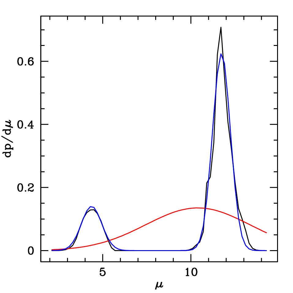
Fig. 1 shows pdfs in distance modulus for three stars. The red curves show Gaussian distributions in distance modulus , while the green curves show distributions that are Gaussian in distance and the blue curves show distributions that are Gaussian in parallax . Given how strongly these three curves differ from one another, especially in the left and centre panels, it is clear that a very particular assumption is being made if one supposes that a star’s distribution of either , or is Gaussian, and if one of these distributions is Gaussian, the other two cannot be.
In each panel of Fig. 1 the black curve shows the computed marginalised pdf in distance modulus , while the red curve shows Gaussian with the same mean and standard deviation as the computed pdf. The green curve shows the pdf which is a Gaussian in distance and has the mean and standard deviation of the computed pdf in distance, while the blue curve shows the pdf which is a Gaussian in parallax and has the mean and dispersion of the computed pdf in parallax. None of the coloured curves can be considered a reasonable representation of the computed pdf. The clear message of Fig. 1 is that it is dangerous to quantify the distance to these stars in the form because this notation implies that a Gaussian pdf adequately approximates the true pdf.
We have derived multi-Gaussian approximations to the pdf in since this variable is physically meaningful for any real number. We write
| (14) |
where , the means , weights , and dispersions are to be determined. We take bins in distance modulus of width , containing a fraction of the total probability taken from the computed pdf, and a fraction of the total probability taken from the multi-Gaussian approximation and consider the statistic
| (15) |
where the weighted dispersion
| (16) |
is a measure of the overall width of the pdf. Our definition of includes the factor to ensure that is unchanged when the width of both the true pdf and our approximation are increased by the same factor: this condition ensures that is a measure of how well the shape of the distribution is fitted. We use in equation (15) rather than the dispersion of the pdf because in some circumstances (double or triple peaked distributions) the dispersion is dominated by the distance between peaks, rather than the widths of the individual peaks themselves, and it is the peaks that should set the scale. A practical difficulty is that is minimised by letting every . Hence instead of minimising , we minimise the alternative statistic
| (17) |
and only use to measure whether the fit is a sufficiently accurate description of the data.


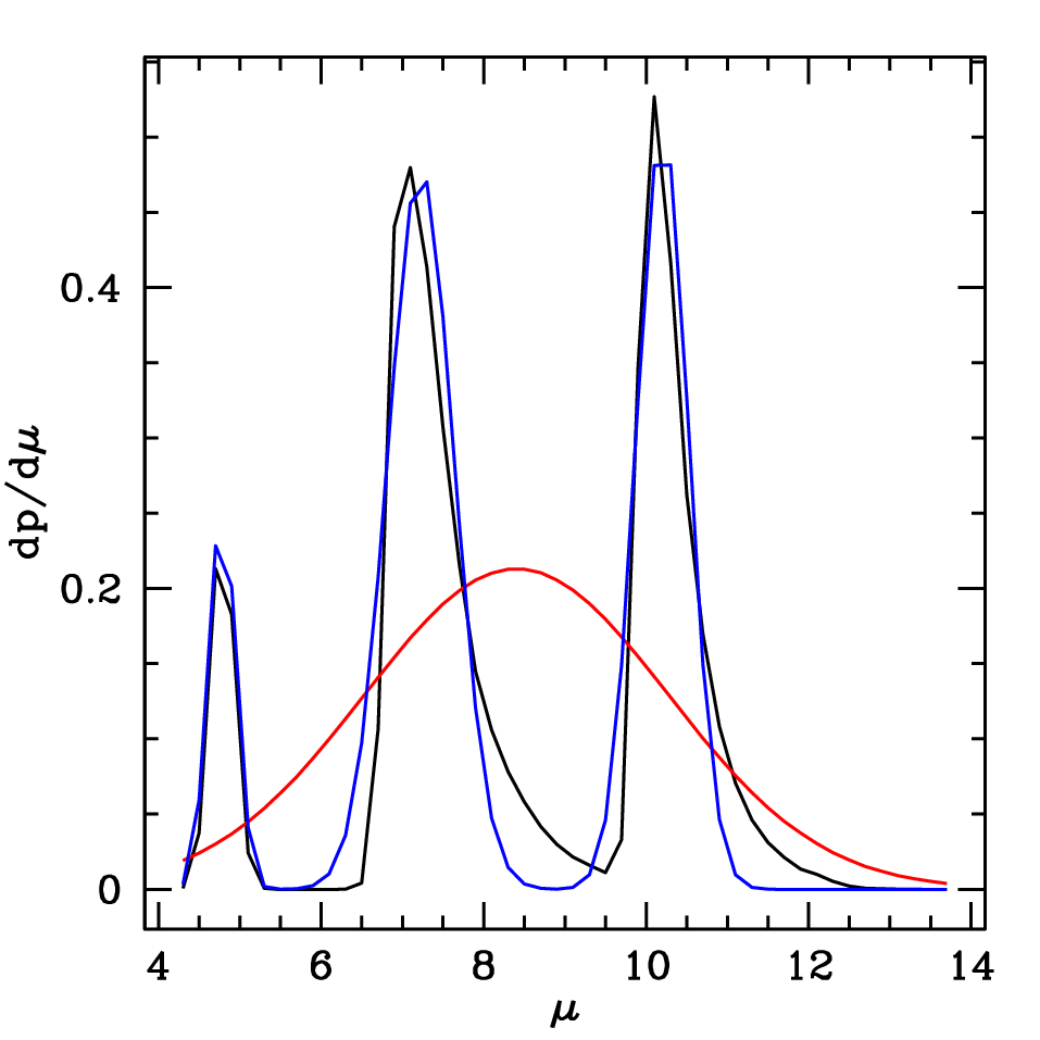
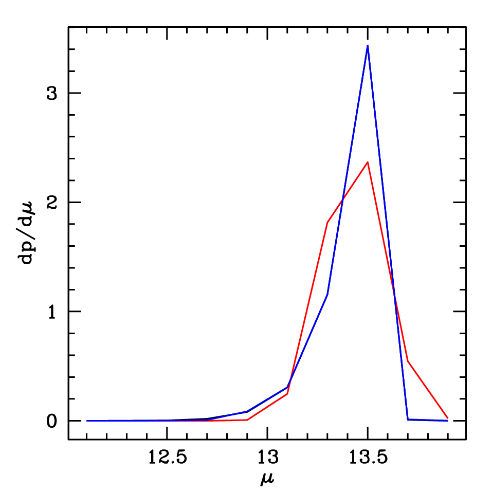
If the value of for a Gaussian with the same mean and dispersion in as that taken from the computed pdf is less than a threshold value , we accept this as an adequate description of the data. This condition holds for around 45 per cent of the RAVE stars. When it fails, we use the Levenberg-Marquardt algorithm to minimise with and several different initial choices for the parameters. We accept this description of the data if it gives and the dispersion of the model is within 20 per cent of that of the complete pdf. The latter condition ensures that we do not accept models that provide an excellent fit to a significant component of the probability but ignore a small but non-negligible component at a different distance. If the two-Gaussian description fails, we fit a three-Gaussian approximation. We reach this stage for around 5 per cent of the RAVE stars because the double-Gaussian approximation is accepted in per cent of cases. Fig. 2 shows the multi-Gaussian models fitted to the pdfs shown in Fig. 1.
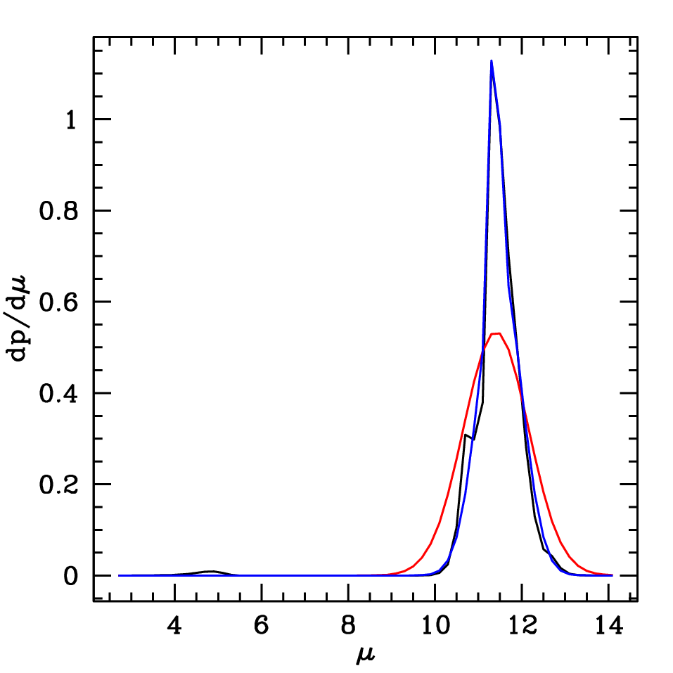
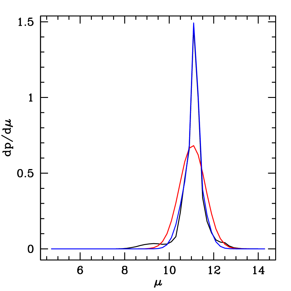
Any fits for which the dispersion of the fitted model differs by more than 20 per cent from that of the data is flagged as possibly inadequate. Approximately four per cent of the models are flagged for this reason. In Fig. 3 we show some typical examples of the flagged models. We see that the problems are in fact minor ones.
4 Hipparcos stars
As in B11, the primary test of the validity of our spectrophotometric distances is provided by Hipparcos stars that are likely to be single stars because in the van Leeuwen (2007) catalogue they have . There are 5614 distinct stars of this type for which we have RAVE parameters, and the mean S/N ratio of their spectra is 84.
The quoted errors on the stellar parameters play a big role in the Bayesian algorithm, and good results are obtainable only with accurate error estimates. When the data were first processed using only the internal error estimates produced by the spectral-reduction pipeline, manifestly inconsistent results for Hipparcos stars were produced. The results were dramatically improved by adding to the internal errors the external errors for various classes of star derived by Kordopatis et al. (2013) and listed in Table 4. The quadrature sums of the internal and external errors prove to be quite similar to the errors adopted by B11, which could not be founded on star-specific error estimates from the old pipeline.
The black points in Fig. 4 show histograms of the discrepancies between Hipparcos parallaxes and expectation values of parallaxes obtained from for three groups of stars: giants (), hot dwarfs () and cool dwarfs. The parallax differences are normalised by the quadrature sum of the formal errors in the Hipparcos data and our adopted errors, so if our procedure were sound and the central limit theorem applied to the data, the histograms would be Gaussians of unit dispersion. This expectation is met to a pleasing extent for hot dwarfs and giants – for the hot dwarfs the mean of the distribution is and the dispersion is and for the giants they are and . Thus on average the parallaxes of the hot dwarfs are slightly too large, while those of the giants are slightly too small and our error estimates are only a shade too small. The results for the smaller number of cool dwarfs are less clear-cut: the mean and dispersion are and implying that our parallaxes are slightly too large and our errors are materially too small.
| stellar type | N | |||
| dwarfs | ||||
| hot, metal-poor | 28 | 314 | 0.466 | 0.269 |
| hot, metal-rich | 104 | 173 | 0.276 | 0.119 |
| cool, metal-poor | 97 | 253 | 0.470 | 0.197 |
| cool, metal-rich | 138 | 145 | 0.384 | 0.111 |
| Giants | ||||
| hot | 8 | 263 | 0.423 | 0.300 |
| cool, metal-poor | 273 | 191 | 0.725 | 0.217 |
| cool, metal-rich | 136 | 89 | 0.605 | 0.144 |
| Hot dwarfs | 1.045 | 1.040 | 0.958 | 1.042 |
|---|---|---|---|---|
| Cool dwarfs | 1.116 | 1.094 | 1.132 | 1.447 |
| Giants | 1.111 | 1.093 | 1.115 | 1.386 |
It is interesting to compute means of the distances ratios. Let
| (18) |
where overbars imply averages of a group of stars and is the distance implied by the expectation value of the distance modulus. Table 5 gives these ratios for hot dwarfs, cool dwarfs and giants. For the hot dwarfs all ratios are pleasingly close to unity, but for both the cool dwarfs and the giants we see that gives a systematically larger distance than , which in turn gives a bigger distance than , which itself gives a bigger distance than , which we take to be the most reliable distance estimator. These biases are easily understood in terms of the weights that each estimator attaches to possibilities of long or short distances. The comparisons with the Hipparcos parallaxes clearly indicates that for stars with wide distance pdfs (cool dwarfs and giants), performs much better than either or .
The red points Fig. 4 show histograms of discrepancies between the Hipparcos parallaxes and parallaxes based on the multi-Gaussian fits to the distance moduli as follows. When a single Gaussian has been fitted, we convert the mean and dispersion of this Gaussian into a parallax and its error by standard formulae. If two or three Gaussians have been fitted, we choose the Gaussian that makes the Hipparcos parallax most probable and convert the mean and dispersion of this Gaussian to a parallax and its error as before. The red histogram for the hot dwarfs is an almost perfect realisation of the unit Gaussian while that for the giants is only marginally less satisfactory than the corresponding black histogram. The red histogram for the cool dwarfs is both significantly displaced to the right and broader than it should be.
Fig. 5 clarifies the situation by splitting the histogram of the cool dwarfs into those with pdfs that have been fitted with a single Gaussian (lower panel) and those with multi-Gaussian fits (upper panel). We see that for the latter stars the crude mean of possible parallaxes is smaller than it should be, and a more satisfactory distribution of spectrophotometric parallaxes is obtained if Hipparcos is used to choose between the Gaussians. The lower panel in Fig. 5 shows that when a cool dwarf has a single-Gaussian pdf, its parallax is systematically over-estimated. When the single- and multi-Gaussian samples are aggregated in Fig. 4, the over-estimated parallaxes of the single-Gaussian stars combine with the under-estimated parallaxes of the multi-Gaussian stars to produce a deceptively satisfactory black histogram. The mean S/N ratio of the Hipparcos stars with single-Gaussian fits is lower than that of the stars with multi-Gaussian fits (51.0 versus 66.5), so one suspects that with poorer data the system loses track of the possibility that the star has left the main sequence.
We test the soundness of the probabilities assigned to each Gaussian component of the pdf by calculating the sums , where depending on which Gaussian component the Hipparcos data points to, and is the weight of that component. Given a large and sample of stars with accurate parallaxes (so the true component is always chosen), should be independent of because when is small, that component will be rarely chosen so will have a small number of large contributions, while a component with large will be chosen often, but each contribution to will be modest. When we compute mean values of for our Hipparcos stars, we find 441/2807 hot dwarfs with two Gaussians fitted, and for these stars we find . Similarly, 615/970 cool dwarfs have two Gaussians and for these stars we find , while 100 cool dwarfs have three Gaussians and for these stars . 934/2015 giants have two Gaussians and these stars yield while 492 giants have three Gaussians and for these stars . These results suggest that the probabilities assigned the various Gaussians are broadly correct although there is a tendency for too little probability to be assigned to the weakest components.
The likely explanation of the neglect of weaker components is that the Hipparcos stars are biased towards nearer stars because stars thought to be near, usually on account of having large proper motions, preferentially entered the Hipparcos Input Catalogue. Consequently, we have tested the constancy of the for a sample in which distant options will have been rather rarely chosen. For the giants the distant option is the more probable one, so it is natural that for these stars Hipparcos chooses the less probable Gaussian more often than one would expect if we had parallaxes for every star in our sample.
Fig. 6 shows the effect of setting for all stars. With reddening neglected, dwarfs must be moved to lower masses to match the observed colours, and the consequent diminution of their luminosities causes them to be brought closer to match the observed magnitudes. The overall effect is to increase the spectrophotometric parallaxes of hot dwarfs by , so those of the hot dwarfs are now on average too large by , while those of the cool dwarfs are too large by . With extinction neglected, giants need to be moved away to diminish their brightnesses so their histogram of moves leftward, and our parallaxes become too small by on average. Thus the Hipparcos stars convincingly validate our procedure for taking into account the effects of dust.
Fig. 7 compares the distribution in the fractional errors in Hipparcos parallaxes (shown in green) with the corresponding errors in our parallaxes: the black points are for the straightforward expectation values of while the red points are for the parallaxes computed from the multi-Gaussian fits to the pdfs in distance modulus. For hot dwarfs the black and red histograms are similar because few of these stars have multi-modal pdfs. They show error distributions that are materially narrower than that from Hipparcos, with most values of falling in the range with a median value of .
For the cool dwarfs the black and red histograms are quite different in that the red histogram shows a substantial population with spectrophotometric parallaxes in error by less that 10% and essentially no stars with errors greater than 35%. The stars with are stars that the spectrophotometry cannot securely assign to dwarfs or giants until astrometric data become available – in the present case a Hipparcos parallax. There will probably be many stars of this type in the Gaia Catalogue. The red histogram for the giants shows a similar if smaller population of stars.
For now we must live with dwarf/giant confusion and the black histograms of parallax errors are most relevant. These show that the spectrophotometric parallaxes of cool dwarfs are not competitive with Hipparcos parallaxes, in contrast to the case of some hot dwarfs and a number of giants, which do have more precise spectrophotometric parallaxes than Hipparcos parallaxes. Thus the competitiveness of the spectrophotometric parallaxes vis a vis Hipparcos parallaxes increases along the sequence cool dwarfs to hot dwarfs to giants in parallel with the increase in the luminosities and thus typical distances of these stars.
| Giants () | ||||
|---|---|---|---|---|
| 69008 | 1.11 | 1.13 | 1.26 | |
| Red Clump | 39900 | 1.04 | 1.04 | 1.09 |
| 28472 | 1.06 | 1.05 | 1.11 | |
| Dwarfs () | ||||
| 22701 | 1.04 | 1.03 | 1.07 | |
| 71641 | 1.04 | 1.04 | 1.08 | |
| 19697 | 1.08 | 1.08 | 1.17 | |
| 27408 | 1.13 | 1.12 | 1.29 | |
5 Distances to all stars
We have examined the statistics of distances to RAVE stars as functions of a cutoff in the S/N of the analysed spectrum and found that dependence on the cutoff S/N is weak. Below we report results obtained for stars with – the mean S/N ratio for such stars that lie closer than is 33.
We have investigated the sensitivity of our distances to the model of the disc used in the prior (eqs 3 and 4) by re-evaluating the distances to every twentieth star in the catalogue with the scale radii and scale heights of both discs multiplied by a factor . The resulting histogram of ratios of the parallax with the revised prior to the parallax with the standard prior peaks sharply at but has a long tail to values with the consequence that the mean of this ratio is . This result shows that, as one would hope, our results are not sensitive to the prior.
Table 6 shows the ratios of the available distance measures for ordinary stars, broken down into giants and dwarfs, with the giants subdivided into stars with lower surface gravity than the red clump ( and ), the red clump itself and stars with higher gravities. We see that in every case the distances are ordered . Moreover, and are discrepant at the 26% level for the highest-gravity giants and coolest dwarfs, while for moderately cool dwarfs these measures are discrepant at the 17% level.
5.1 Kinematic distance corrections
Schönrich et al. (2012; hereafter SBA) describe a technique that uses the kinematics of stellar populations to identify and correct systematic errors in distances, and we can use this technique to determine which of our discrepant distance estimates is most reliable, and potentially to correct the most reliable measure for any systematic bias.
The corrections of SBA are based on the assumption that one knows roughly how the velocity ellipsoid is oriented at each point in the Galaxy, and that the only mean-streaming motion is azimuthal circulation at a speed , where is an unspecified constant and is a function one chooses. We adopt
| (19) |
which has an appropriate form, but the results are very insensitive to the choice of : essentially unchanged results are obtained with . The algorithm involves converting heliocentric velocities to Galactocentric velocities and thus requires assumptions regarding the Galactocentric velocity of the Sun and the distance to the Galactic centre. We assume that , that the local circular speed is , and that the Sun’s velocity with respect to the Local Standard of Rest is (Schönrich et al., 2012). There is very little sensitivity to the value of . The azimuthal direction is assumed to be a principal axis of the velocity ellipsoid, while the latter’s longest axis is tilted with respect to the plane by angle , where is a parameter.
The corrections exploit pattern on the sky of correlations between the local Cartesian velocity components that are introduced by distance errors. To assess the magnitude of these correlations one has first to correct the raw correlations for contributions from sources other than distance errors. The most important such source is observational errors in the proper motions, so knowledge of the magnitude of these errors is needed for the correction.

Proper motions for RAVE stars can be drawn from several catalogues. Williams et al. (2013) compares results obtained with different proper-motion catalogues, and on the basis of this discussion we decided to work with the PPMX proper motions (Röser et al., 2008) because these are available for all our stars and they tend to minimise anomalous streaming motions. Fig. 8 shows a histogram of the errors for RAVE stars given in the PPMX catalogue. It shows that there is a fat tail in the error distribution, and one may show that this tail should not to be taken at face value because when one calculates the velocity dispersions of all the RAVE stars in spatial bins that are further than from the Sun, the dispersions are often smaller than the contribution expected from proper-motion errors alone. This paradox disappears if one cuts stars with errors in one component of proper motion greater than , and we impose this cut throughout the SBA analysis. The only class of stars that is significantly depleted by this cut is that of the very cool dwarfs, which shrinks from stars to stars. This cut reduces the rms error in one component of proper motion to .
A second source of correlations that complicate the SBA analysis is rotation of the velocity ellipsoid’s principal axes as one moves around the Galaxy, and a model of the velocity ellipsoid is used to correct for this effect. The final product is the factor by which all distances must be contracted (or expanded if ) for all correlations between , and to be accounted for by a combination of observational errors and rotation of the principal axes of the velocity ellipsoid.
SBA give two formulae for corrections, one, , involving “targeting” and one, , using as a target. Because the latter is independent of azimuthal streaming, it is the simpler and more reliable. Their equations (19) and (38) give the and correction factors, respectively, after the raw covariances have been corrected for observational errors using their equations (22) and (25).
| Giants () | ||||
| 0.304 | 0.323 | 0.134 | 0.248 | |
| Red Clump | 0.311 | 0.332 | 0.160 | 0.249 |
| 0.310 | 0.348 | 0.453 | 0.676 | |
| Dwarfs () | ||||
| 0.295 | 0.295 | -0.270 | -0.210 | |
| 0.312 | 0.312 | -0.081 | -0.037 | |
| 0.286 | 0.286 | -0.064 | -0.027 | |
| 0.306 | 0.306 | -0.026 | 0.043 | |
| Giants () | ||||
| 0.203 | 0.203 | 0.066 | 0.185 | |
| Red Clump | 0.157 | 0.157 | 0.114 | 0.148 |
| 0.100 | 0.130 | 0.210 | 0.334 | |
| Dwarfs () | ||||
| 0.220 | 0.207 | -0.270 | -0.210 | |
| 0.217 | 0.217 | -0.081 | -0.037 | |
| 0.227 | 0.247 | -0.064 | -0.027 | |
| 0.217 | 0.217 | -0.050 | 0.041 | |
From the RAVE data we have extracted correction factors to the distance estimator for the three types of giants and four types of dwarf listed in Table 6. The code used to determine the corrections was tested as follows. For each star in a class, the measured velocities were replaced by values chosen from a triaxial Gaussian velocity ellipsoid that has dispersions around systematic rotation at . Most tests were run with the orientation of the principal axes determined by setting , but excellent results are obtained with other plausible values of , including zero. Likewise, the outcome of the code tests is not sensitive to the adopted dispersions . Next proper motions and line-of-sight velocities are calculated from the model velocities, and Gaussian observational errors are added with the dispersions that are given in the PPMX catalogue. Then the stars are moved along their lines of sight to points more distant by a factor and their components are re-evaluated from the proper motions. In this way we obtain a catalogue of phase-space positions for a population of objects whose distances have been over-estimated by a factor . The SBA algorithms are then used to infer from this catalogue the value of .
The first two numerical columns of Table 7 show the fractional distance excesses and obtained by targeting and when distances to the stars have been over-estimated by a factor with . Consequently, ideally we would have for all star classes. For this expectation is borne out for all classes to better than , and for the dwarfs it is similarly for . For the giants is up to larger than it should be, a result which reflects the breakdown of the approximations made by SBA when dealing with more distant stars.
The final two columns of Table 7 show the fractional distance excesses and for the seven classes of RAVE stars using the measured distances and velocities when is used as the distance measure. For the giants the differences between and are in the same sense () as in the tests but they are larger than in the tests. The cause of this difference is not obvious, but one suspects a major contributor is the well-known existence of clumps of stars in the plane (Dehnen, 1998; Famaey et al., 2005; Antoja et al., 2012), which conflict with the assumption of simple azimuthal streaming that is fundamental to SBA’s derivation of the formula for . Since prominent clumps are absent from the distribution of Hipparcos stars in the and planes (Dehnen, 1998), is expected to be a more reliable diagnostic of distance errors than . Table 7 then suggests that over-estimates distances to high-gravity giants and red-clump stars by , and gives distances to dwarfs that are too small by factors that rise from at the cool end rising to at the hot end.
In selecting stars for inclusion in the SBA analysis we have imposed a limit on the reported distance, and the results one obtains for both the test and with the real data depend on the value chosen for . Table 7 is based on the choice . Table 8 is based on and the results of tests reported in the first two numerical columns of this table differ from those reported in the corresponding columns of Table 7 in that the distances to stars were increased by a factor where is now a Gaussian random variable with mean and dispersion . The test results are fairly satisfactory for the dwarfs in that both and have values within of the true value, . The test results for the giants are decidedly less satisfactory in that the values are too small by an amount which increases with the typical luminosity within a class. It is easy to understand why this is so: stars that happen to get a large fractional distance increase are liable to be pushed beyond whilst stars that have their distances decreased can enter the sample from beyond , and the SBA algorithm correctly infers that on average the stars in the analysed sample have small distance over-estimates even though in the population as a whole stars have larger distance over-estimates. Clearly, for this phenomenon to be important the catalogue needs to contain many stars that really are at distances . The dwarfs do not satisfy this condition, but the low-gravity giants very much straddle the distance cut.
Comparing columns 3 and 4 of Table 8 with the corresponding column of Table 7 we see that reducing from to has only a modest effect on the values for dwarfs and a significant effect on giants. The values of giants decrease significantly for all three classes, but the final factors still increase with decreasing gravity contrary to the tendency seen in the test, so we really must be over-estimating distances to the lowest-gravity (and most luminous) giants. A possible explanation is that we are using stellar parameters obtained under the assumption of Local Thermodynamic Equilibrium (LTE). The validity of LTE decreases with , and when non-LTE effects are taken into account, the recovered gravity of a giant star increases (Ruchti et al., 2013), and the predicted luminosity decreases, bringing the star closer.


The squares in Fig. 9 show the values of obtained when the giants are grouped by and the dwarfs are grouped by – in each case the SBA algorithm is used on 15 bins of stars at with equal numbers of stars in each bin, and all bins statistically independent. The triangles show the analogous ratios of our distance to that implied by the Hipparcos parallax. The curves show fifth-order polynomial fits to all the points. The squares and triangles tell the same story from a qualitative perspective: along the sequence of giants there is a steady increase in the tendency to over-estimate distances as one moves to lower gravity (and higher luminosity), while the dwarfs show a clear trend towards distance over-estimation with falling with the exception of the coolest bin, which shows marked distance under-estimates. The SBA points for dwarfs tend to lie below those from Hipparcos, so SBA and Hipparcos disagree about the value of at which our distances are unbiased.
Our tests suggest that should be a reliable guide to any systematic errors in the distances to our dwarf stars. The situation regarding the giant stars is less clear because the values are biased low unless is large enough to encompass most of the stars in the catalogue. Unfortunately, the more distant stars are, the more sensitive the returned value of becomes to restrictive assumptions regarding the pattern of mean-streaming and random velocities in the Galaxy and some approximations. The value of is less sensitive to these issues and therefore more reliable, but its sensitivity to is worrying. A further blow to the credibility of will emerge below from an analysis of the red-clump stars.
5.1.1 Kinematic corrections to multi-Gaussian pdfs
SBA assume that one is working with a simple distance estimator, while in Section 3 we saw that our most complete information is contained in a distance pdf. Can we use a kinematic analysis to refine these pdfs?
The SBA algorithm involves several sample averages such as , where and are quantities that depend on the distance to each star. In our analysis above we evaluated these for just one distance, but given a pdf it is straightforward to replace by the expectation value of :
| (20) |
These expectation values are then averaged over the sample to produce the sample averages , etc., that appear in the SBA formalism. Thus is straightforward to use the pdfs to calculate a kinematic correction factor such as .
It is less clear how one should modify the pdf in light of a non-zero value of . We have experimented with two possibilities.
- (i)
Move the centres of all the Gaussians to larger or smaller distance moduli until, . This procedure produces results that are rather similar to, but slightly less convincing than, those obtained without the pdfs.
- (ii)
When a star has more than one Gaussian in its pdf, modify the probabilities (eqn. 14) associated with the two most probable Gaussians. This procedure is appropriate if the Bayesian algorithm has correctly identified the two model stars that an observed star could be, but, perhaps driven by a faulty prior, has assigned inappropriate odds to the options. We now report results obtained with this procedure.
We make the probabilities and in equation (14) a function of a variable through
| (21) |
where at the outset we fix to be the total probability associated with the two most probable options. Then we make , which is confined to the range , a function of a variable that can span the whole real line, through
| (22) |
The original values of determine starting values for and . If the kinematic analysis has returned , implying that distances need to be shortened and the first Gaussian describes a nearer option than the second, then we lower by subtracting from – the factor 5 is arbitrary: smaller values lead to slower convergence of the iterations but larger values can cause the iterations to undergo diverging oscillations. If, conversely, , we need to increase and so we add to .
| Giants () | |||
| 2.16 | 0.403 | 0.004 | |
| Red Clump | 24.85 | 0.906 | 0.858 |
| 5.55 | 0.290 | 0.134 | |
| Dwarfs () | |||
| 8.22 | -0.252 | -0.247 | |
| 0.39 | -0.015 | -0.009 | |
| 0.55 | 0.030 | 0.004 | |
| 1.99 | 0.247 | 0.005 | |
In Table 9 shows results obtained by iterating up to six times or until . The first numerical column gives the mean of for all stars that have more than one Gaussian. A value greater than implies that all available probability has been driven into whichever Gaussian will reduce . For the giants this condition is reached after about four iterations and is signalled by successive values of becoming nearly identical. The second column gives the initial value of and the third column gives the value of at the end of the iterations. We see that in the case of the highest-gravity giants, adjusting the has reduced to the target value, but that there is insufficient ambiguity in the nature of the clump stars and the low-gravity giants to get below the target value.
There is very little ambiguity in the nature of the hottest dwarfs, so the procedure makes no significant progress in eliminating the tendency for their distances to be under-estimated.
The procedure succeeds with the remaining dwarfs: for all three classes is reduced to below the target value, and the modest values of given in the first numerical column show that this is achieved without driving all the probability into one option.
From this analysis we conclude that there is sufficient ambiguity in the nature of stars that are cooler that and have to account for non-zero values of the SBA factor but too little ambiguity in the nature of hotter dwarfs and low-gravity giants to account for non-zero .
5.2 Absolute magnitude of the red clump
Helium-burning stars in the red clump have frequently been used as standard candles (Cannon, 1970; Pietrzynski, 2003, e.g.). Recently Williams et al. (2013) used clump stars in the RAVE survey to analyse the velocity field around the Sun, and reviewed our knowledge of the absolute magnitudes of these objects and the possibility that they depend on age and metallicity. They identified clump stars as those satisfying the cuts and , where was taken from the vDR3 pipeline (Siebert et al., 2011). We use the same colour range but a narrower band in and with gravity taken from the vDR4 pipeline (Kordopatis et al., 2013).
Fig. 10 shows the distributions of - and -band absolute magnitudes for distance of clump stars. The distributions are satisfyingly narrow – each has a standard deviation of – but they are skew, so while their means lie at and their peaks lie at and . These magnitudes are in the SAAO system: using the formulae of Koen et al. (2007) to convert to the 2MASS system we find the mean of to be . The sample was restricted by but increasing the distance cutoff to only changes the mean absolute magnitudes to and . For comparison Laney et al. (2012) determined and from a sample of 191 Hipparcos stars, and (Williams et al., 2013) used calibrations in which the 2MASS absolute magnitudes were , and . In the last calibration the decrease in luminosity with increasing distance from the plane reflects the expected increasing age and decreasing metallicity of clump stars. However, the age-metallicity sensitivity of the absolute magnitude is expected to be smallest in the K band (Salaris, 2013, e.g.). Several issues require discussion when considering why our values are mag fainter than those of Laney et al.
- •
One might argue that the figures given above actually under-estimate the scale of the conflict with Laney et al. (2012) (and many similar values in the literature) because we ought to have corrected our values for the systematic distance over-estimates implied by the upper panel of Fig. 9. When this is done (using the red curve) we obtain and ; since we have moved the stars nearer, we conclude that they are less luminous.
- •
The study of Laney et al. (2012) involved obtaining new photometry for their Hipparcos stars because the 2MASS photometry of Hipparcos red clump stars, which have bright apparent magnitudes, is affected by saturation, which makes them appear fainter than they really are. Unfortunately, only four of our stars were measured by Laney et al. For these stars Laney et al. obtained magnitudes brighter than the 2MASS values by amounts in the range , but their and values are not clearly brighter than the 2MASS values, which suggests that saturation in 2MASS is mainly confined to the band. Interestingly, the Bayesian algorithm assigns an anomalous extinction () to the star (Hipp 32222) that shows by far the strongest saturation effects, presumably because a high extinction can explain the unexpectedly faint magnitude given the spectroscopically determined . From this rather fragmentary evidence we infer that the effects of saturation on the 2MASS magnitudes might cause us to make the nearest clump stars under-luminous by mag. The triangles in Fig. 9 suggest on the contrary that we have found these stars to be over-luminous by mag.


Figure 11: Density of stars on a logarithmic scale for two metallicity ranges in the () plane together with Padua isochrones for a metal-rich populations. The left panel is for and the right panel is for . - •
Are the red clump stars in our sample correctly identified? Fig. 11 shows the density of stars in the plane for two metallicity ranges. In both panels peaks in density are apparent near the theoretical locations of core helium-burning stars, These peaks are captured by our selection criteria and . The core helium-burning model star that sits at the centre of the red circle has , and , in agreement with the empirical data of Laney et al. (2012).
This discussion explains why our raw distances imply absolute magnitudes for clump stars that differ little from the empirical value of Laney et al., and why these distances are only slightly larger than the Hipparcos parallaxes imply. The puzzle remains that the SBA kinematic analysis points to our distances being too large. For the SBA analysis to be correct, we would require both that the stellar models were too luminous and the Hipparcos stars to be misleading, perhaps because they are nearby and therefore anomalously young and have atypical chemistry. Consequently, we set the SBA correction factors aside for the moment but in a companion paper (Binney et al., 2013) we will return to this issue in the context of dynamical Galaxy models.
Table 6 shows that is always the shortest of our distance measures, and given the suggestion from the SBA analysis that even this measure might be too long, we do not present an SBA analysis of distances based on or . However, such analyses do confirm that these measures over-estimate distances to all classes of star by even larger factors than does, so there is no case to be made for using them.


5.3 Effective temperature absolute magnitude diagrams
Fig. 12 shows effective temperature absolute-magnitude diagrams for high-latitude () stars created either (a) using to assign a single distance to each stars (left panel) or (b) spreading each star in according to the multi-Gaussian fit to its pdf in distance modulus. The red octagon centred on shows the location of the Sun in the effective temperature absolute magnitude diagram.
The red clump is prominent in both panels but the horizontal branch extends further to the blue when the pdfs are used as a consequence of eliminating the messy scatter of stars in the left panel between the horizontal branch and the main sequence. Using the pdfs similarly eliminates the unphysical scatter of stars inside the turn-off curve. In both diagrams vertical stripes are evident, especially at the coolest temperatures: these are a legacy of the use by the pipeline of the DEGAS decision-tree routine to identify template spectra (Kordopatis et al., 2013). This artifact is enhanced because we have smeared stars in but not in , as we should have done for consistency.


Fig. 13 shows effective temperature absolute-magnitude diagrams for two slices through the Galaxy: or . For these plots we used the multi-Gaussian representations of pdfs to spread stars in distance modulus and thus in . At the main sequence, subgiant and giant branches show up nicely, and the red clump is extremely sharp. More than away from the plane the lower main sequence has disappeared and giant branch becomes more strongly populated because the volume surveyed is much larger.
| Cluster | ||||||||||||
|---|---|---|---|---|---|---|---|---|---|---|---|---|
| Blanco 1 | 5.5 | 0.01 | 7.80 | 9.59 | 269 | 4 | 1.61 | 23 | 1.07 | 1.15 | 1.13 | 0.87 |
| NGC 2422 | 3.6 | 0.07 | 7.86 | 8.82 | 490 | 0 | 13 | 1.09 | 1.09 | 1.08 | 0.85 | |
| Alessi 34 | 15.4 | 0.18 | 7.89 | 9.58 | 1100 | 24 | 1.20 | 0 | 1.20 | 1.82 | 3.71 | |
| ASCC 69 | 14.0 | 0.17 | 7.91 | 9.51 | 1000 | 30 | 1.63 | 2 | 0.84 | 1.58 | 2.11 | 4.87 |
| NGC 6405 | 2.8 | 0.14 | 7.97 | 8.89 | 487 | 0 | 12 | 0.94 | 0.94 | 0.90 | 0.71 | |
| Melotte 22 (Pleiades) | 4.6 | 0.03 | 8.13 | 9.39 | 133 | 2 | 1.11 | 35 | 1.09 | 1.09 | 1.11 | 0.93 |
| NGC 3532 | 7.1 | 0.04 | 8.49 | 8.95 | 486 | 1 | 1.71 | 17 | 1.23 | 1.26 | 1.24 | 0.97 |
| NGC 2477 (M93) | 5.7 | 0.24 | 8.78 | 9.29 | 1300 | 45 | 0.91 | 3 | 1.02 | 0.92 | 1.13 | 1.27 |
| Hyades | 5.7 | 0.01 | 8.80 | 9.70 | 46 | 0 | 31 | 1.08 | 1.08 | 1.08 | 1.00 | |
| NGC 2632 (Praesepe, M44) | 3.8 | 0.01 | 8.86 | 9.48 | 187 | 0 | 34 | 1.14 | 1.14 | 1.12 | 1.03 | |
| NGC 2423 | 2.7 | 0.10 | 8.87 | 8.96 | 766 | 3 | 1.36 | 17 | 0.99 | 1.05 | 0.99 | 1.17 |
| IC 4651 | 2.6 | 0.12 | 9.06 | 9.30 | 888 | 7 | 1.03 | 5 | 0.68 | 0.87 | 0.87 | 1.00 |
| NGC 2682 (M67) | 6.6 | 0.06 | 9.41 | 9.74 | 908 | 32 | 0.74 | 12 | 0.65 | 0.72 | 0.74 | 0.78 |
6 Cluster stars
By searching for stars that have suitable sky coordinates and line-of-sight velocities that agree with a cluster convergence point, we have identified RAVE stars in 15 open clusters. NGC 3680 has just one RAVE star so we cannot analyse its statistics. Table 10 lists the remaining clusters with RAVE stars in order of increasing age, giving for each cluster the values of several quantities from the literature. The values given are taken from Dias et al. (2002) with the exception of the Hyades, where we used Perryman et al. (1998).
Columns 7 and 8 give the number of giants in our sample and the ratio of their mean value of to the distance listed in Table 10. Columns 9 and 10 give the same data for dwarfs, and column 11 gives the overall mean of for cluster stars divided by the literature distance. A tendency for the giants to over-estimate distances is evident, particularly in the younger clusters such as Alessi 34 and ASCC 69. The distances inferred for dwarfs are generally in good agreement with the literature values, but significant under-estimates are evident in the cases of the oldest clusters, IC 1651 and NGC 2682 (M67). The penultimate column gives the mean value of divided by the literature distance when extinction is assumed to be zero. Setting shortens distances to dwarfs and lengthens those to giants and for a few clusters the results with no dust are markedly worse but neglecting dust has little impact on most clusters.
Column 5 gives the the mean inferred value of the logarithm of age (in years) and comparing these values with the literature values in column 4 we see little sign of correlation with the result that stars in younger clusters are being presumed much older than they really are. This phenomenon reflects the fact that dating an isolated star is enormously harder than dating a cluster of coeval stars. Clearly poor ages will bias the recovered distances so in the last column of Table 10 we give the mean values of divided by the literature distance when distances are determined under the strong age prior
| (23) |
This cluster-specific age prior improves the accuracy of mean distances to stars in clusters older than , but has an unfortunate effect on the distances to stars in younger clusters.
Fig. 14 shows histograms of distances to stars in 12 of the 13 clusters listed in Table 10; the red histograms are for our standard distances and the blue histograms are for distances obtained under the strong cluster-specific prior. The numbers in brackets after the cluster names in the top left corner of each panel give the number of giants and dwarfs in that cluster. The top panel of Fig. 15 shows the corresponding plot for NGC 2682 (M67). We see that the strong age prior shortens distances to dwarfs and lengthens those to giants in a way that is moderate and beneficial in clusters as old as the Melotte 22 (Pleiades) but unhelpful in younger clusters. The red histograms are generally quite satisfactory.


7 Repeat observations
We have more than one spectrum for stars and can form independent pairs of measurements for the same dwarf star and independent pairs of measurements for the same giant star. Fig. 16 shows histograms of the discrepancies between these measurements when normalised in two ways. In the upper panel the difference in is divided by the mean parallax, while in the lower panel it is divided by the quadrature-sum of the uncertainties of the measurements. The median fractional parallax discrepancy is for giants and for dwarfs – it is easy to show that these values apply also to the discrepancies in distances . The dispersions of the parallax discrepancies normalised by the formal uncertainties is for giants and for dwarfs. That these numbers are significantly smaller than unity emphasises that much of the error is external and does not derive from noise in the spectrum.


8 Estimated extinctions
As with distances, the Bayesian algorithm determines a probability distribution for possible extinctions to each star, and one has to consider how best to reduce this distribution to a single value for the extinction. For the reasons given in Section 2 the code marginalises over extinctions by integrating with respect to rather than integrating with respect to directly. Consequently a natural quantity to output is , and we use as our estimator of the extinction. places less weight on high extinctions than does .
Fig. 17 shows that different spectra yield the same value for to high precision: the dispersion in the differences divided by the quadrature sum of the uncertainties is only for giants and for dwarfs. This result is to be expected because depends strongly on the photometry, and we only change the spectrum between determinations of .
Fig. 18 shows in red the distribution of extinctions to Hipparcos stars; the blue points show the distribution of the prior values of the extinction to the final locations of the stars. Since the red and blue points follow very similar distributions, on average our recovered extinctions coincide well with our priors. This finding could indicate either that our priors are accurate guesses of the actual extinction, or that the extinction to an individual star cannot be determined from the data we have. We know that the data are adequate because when we took the priors from the smooth model (11) normalised in an average sense by the Schlegel et al. reddenings, the recovered values of were systematically smaller than the prior values. Thus the data suffice to shift the recovered values away from a poor prior. Presumably the Hipparcos stars lie in directions of anomalously low extinction, an effect that is captured when the extinction is estimated to be the fraction of the measured extinction to infinity that is expected to lie within distance .
For hot dwarfs most values of lie in [so lies in ], while a significant fraction of cool dwarfs have as we would expect given that some of these stars are quite close. The distribution of values of for giants peaks around but has a long tail extending out to as we expect for stars that can be quite distant.
Fig. 19 shows histograms of the differences between our estimated extinctions to stars in the complete sample and the value of the prior on extinction to the star’s proposed location. The red, blue and black histograms are for stars that lie in three ranges of Galactic latitude . The means of all the two highest-latitude histograms are satisfyingly close to zero. The mean of the histogram for deg is negative () implying that the dust model slightly over-estimates extinctions to low-latitude stars.
Fig. 20 shows the relationship between extinction and distance for hot dwarfs (), cool dwarfs and giants () in the full RAVE sample. In addition to showing the extent of the relation between distance and extinction, these plots show how the three classes of star are distributed in distance. The ridge line through the distribution of giants has a slope mag/kpc, while that through the distribution of cool dwarfs has a slope mag/kpc. For comparison, the traditional relation for paths near the mid-plane is kpc (Binney & Merrifield, 1998, e.g.). Since most of our sight lines move away from the mid-plane, they naturally have lower values of extinction per unit length. Moreover, our samples are subject to the already-noted observational bias against stars high extinctions, and this bias particularly concentrates the giants at high latitudes, where extinction per unit distance is low.
The red points in Fig. 21 show for each cluster the distribution of , where is 3.1 times the cluster’s literature value of . The blue points show the corresponding distributions of the values obtained by replacing by the prior extinction at . For all clusters the red and blue points have similar distributions, which suggests that the priors are reasonable. In light of this result, it is striking (a) how broad the distributions are, and (b) that in four clusters (Melotte 22, Hyades, NGC 2632 and NGC 2682) the literature extinction lies off one wing or the other of the distribution. These findings call into question the very concept of a cluster-wide characteristic extinction, and suggest that if one must choose a single characteristic extinction, the literature value may be a poor choice.
9 Conclusions
We have extended the Bayesian approach to distance determination of Burnett & Binney (2010) to allow for extinction and reddening and to deliver pdfs in distance modulus in addition to expectation values of three distance measures, distance , distance modulus and parallax .
We have fitted each star’s pdf in distance modulus with a sum of up to three Gaussians. A single Gaussian provides a good fit to about 45 per cent of the pdfs, two Gaussians provide a good fit to most of the remaining pdfs, so just 5 per cent of the pdfs require three Gaussians for a good fit. When these Gaussian decompositions are used to make Hess diagrams by splitting each star’s contribution to the density into one, two or three parts at the luminosity associated with the centre of each Gaussian component, the diagram becomes significantly sharper as the man-sequence turnoff and the horizontal branch emerge clearly. This phenomenon indicates that multi-modal pdfs are associated with stars that could be upper main-sequence stars or blue horizontal-branch stars, or could be lower main-sequence stars or subgiants.
For every class of star examined, we find that , a phenomenon that arises because these distance measures weight differently the possibilities that a given star is far or near. The differences between these distance measures are least for hot dwarfs and red-clump stars, and greatest for very cool dwarfs () high-gravity giants () because hot dwarfs and red-clump stars have quite narrow pdfs in distance while the dwarf/giant ambiguity causes cool dwarfs and high-gravity giants to have broad pdfs in distance.
The RAVE survey encompasses Hipparcos stars. Histograms of the difference between our values of and the Hipparcos parallaxes normalised by the quadrature sum of our errors and the Hipparcos errors come close to the ideal of a unit Gaussian of zero mean in the cases of warm dwarfs () and giants (), so not only are our parallax estimates fairly reliable, but our error estimates are reasonable. The situation regarding the smaller sample of cool dwarfs is unsatisfactory. The majority of these stars require multi-Gaussian fits to their pdfs. When a Hipparcos parallax is available, it agrees within the errors with one of the Gaussians as one would wish. But the single Gaussians fitted to a minority of cool dwarfs yield parallaxes that are significantly larger than the Hipparcos parallaxes. Thus our ability to determine distances to cool dwarfs is rather limited.
For giants our parallaxes are competitive with those of Hipparcos, but for cool dwarfs errors on Hipparcos parallaxes are smaller than the errors on ours by a factor .
The good agreement between our parallaxes and the Hipparcos parallaxes, suggests that is our most reliable estimator of distance, a conclusion we were able to confirm subsequently. Hence we have concentrated on assessing the accuracy of the distance estimator .
The Hipparcos stars in the RAVE survey reveal (Fig. 9) a tendency for our distances to the hottest dwarfs to be too small, while our distances to dwarfs with are too large by about the same amount. Our distances to the coolest dwarfs are 20–30% too small. The Hipparcos stars reveal that our distances to giants are too large by a factor that increases smoothly with decreasing from unity at to at the lowest gravities. This phenomenon may reflect our use of stellar parameters obtained under the assumption of LTE. However, it should be noted that Kordopatis et al. (2013) excise the cores of strong lines, where non-LTE effects will be most prominent.
The values of the kinematic corrections obtained by the method of Schönrich et al. (2012) for all the giants and dwarfs in the RAVE sample confirm the results from the Hipparcos stars: is a more reliable distance estimator for cool stars than and for dwarfs the ratio of to the true distance increases with decreasing except below , where it drops abruptly. For dwarfs the SBA kinematic indicators agree moderately with each other and suggest that our distances tend to be too short by an amount that decreases with from at the hot end to perfection at . The shape of the plot of the ratios of our distance to true distance agrees perfectly with the Hipparcos results, but there is a small vertical offset between the curves.
For giants has a tendency to be too large, by an amount that emerges equally from the Hipparcos results and the SBA kinematic corrector . The ratio of our distance to the true distance increases with decreasing from at the high-gravity end to at the low-gravity end. Unfortunately, the Hipparcos results are of course confined to and the SBA analysis proves sensitive to the upper limit on the distances of stars we use in the analysis. Moreover, for stars with the two SBA factors disagree with each other. Therefor it is hard to assess the accuracy of our distances to stars at , which tend to be luminous low-gravity giants. However, the indications are that we are over-estimating these distances by .
We have identified red-clump stars by cuts in the plane and find that a histogram of these stars’ values of is narrow and peaks mag fainter than the standard magnitude. The origin of this offset is unclear. If we accept the indications from both the Hipparcos stars and the SBA analysis that we systematically over-estimate distances to giants, the offset is made significantly larger: mag under-luminous.
We have identified 364 RAVE stars in 15 open clusters. Our standard distances generally form a satisfyingly narrow distribution with the cluster’s literature distance almost always within one standard deviation of the distribution’s mean. There is a clear tendency for the giants in any cluster to be assigned distances that are larger than the distances assigned to the cluster’s dwarfs. In the oldest clusters, IC 4651 and NGC 2682 (M67), the dwarf distances are only of the cluster distance, but in the other clusters the dwarf distances appear about right.
The data barely constrain the ages of stars. Consequently, our standard distances are based the assumption that stars are quite old, older than the ages of many of the clusters we have studied. Curiously, using a prior on ages that enforces the cluster’s literature age produces a more satisfying histogram of distances only for clusters older than Melotte 22 (the Pleiades).
The data do contain sufficient information to place significant constraints on the extinctions of stars – we know this because the extinctions we first derived were systematically lower than the priors we then employed. This phenomenon led to improved priors and our extinctions now scatter nearly randomly around the prior values. Since extinction varies discontinuously from one line of sight to the next on account of the fractal nature of the ISM, and we do not have a sample of stars with accurately determined extinctions, it is hard to test the validity of our extinctions. Our results for clusters indicate that different stars in the same cluster generally have significantly different extinctions, and that the mean extinction of stars in a given cluster often differs significantly from the cluster’s literature value.
The distances we derive from different spectra of the same star are entirely consistent with one another and imply that noise in the spectrum contributes less that half the uncertainty in the derived distance.
This work could and should be significantly improved in three ways. First, photometry in optical bands is now available for most of our stars from the APASS survey (Henden et al., 2012). Use of this photometry would sharpen constraints on some combination of and . Second, the stellar models used here are now a few years old and should be updated and extended. Inclusion of -enhanced stars with lower metallicities should improve accuracy for stars that are far from the plane. Moreover, we could now use models for which magnitudes in the 2MASS system have been directly computed rather than obtained by transformation of magnitudes in the Johnson-Cousins system. Third, stellar parameters that include corrections for non-LTE effects as discussed by Ruchti et al. (2013) may yield improved distances, especially to luminous giants. Distances based on extended photometry and models will be made available on the RAVE website as soon as possible.
Acknowledgements
We thank the referee for a meticulous reading of the submitted version and many useful suggestions for improvement.
Funding for RAVE has been provided by: the Australian Astronomical Observatory; the Leibniz-Institut für Astrophysik Potsdam (AIP); the Australian National University; the Australian Research Council; the French National Research Agency; the German Research Foundation (SPP 1177 and SFB 881); the European Research Council (ERC-StG 240271 Galactica); the Istituto Nazionale di Astrofisica at Padova; The Johns Hopkins University; the National Science Foundation of the USA (AST-0908326); the W. M. Keck foundation; the Macquarie University; the Netherlands Research School for Astronomy; the Natural Sciences and Engineering Research Council of Canada; the Slovenian Research Agency; the Swiss National Science Foundation; the Science & Technology Facilities Council of the UK; Opticon; Strasbourg Observatory; and the Universities of Groningen, Heidelberg and Sydney. The RAVE web site is at http://www.rave-survey.org.
References
- Antoja et al. (2012) Anotoja T., Helmi A., Bienaymé O., Bland-Hawthorn J., & the RAVE collaboration, 2012, MNRAS, 425, L1
- Arce & Goodman (1999) Arce H.G. & Goodman A.A., 1999, ApJ, 512, L135
- Aumer & Binney (2009) Aumer M. & Binney J.J., 2009, MNRAS, 397, 1286
- Bertelli et al. (2008) Bertelli G., Girardi L., Marigo P., Nasi E., 208, A&A, 484, 815
- Binney (2011) Binney J, 2011, Prama, 77, 39
- Binney et al. (2013) Binney J., & the RAVE colaboration, 2013, to be submitted
- Binney et al. (1997) Binney J.J., Gerhard O.E., Spergel D., 1997, MNRAS, 288, 365
- Binney & Merrifield (1998) Binney J., Merrifield M., 1998, “Galactic Astronomy”, Princeton University Press, Princeton
- Breddels et al. (2009) Breddels M.A., et al., 2010, A&A, 511, 90
- Burnett & Binney (2010) Burnett B & Binney J., 2010, MNRAS, 407, 339
- Burnett et al. (2011) Burnett B., Binney J. & the RAVE collaboration, 2011, A&A, 532, 113
- Cannon (1970) Cannon R.D., 1970, MNRAS, 150, 111
- Carollo et al. (2009) Carollo D., Beers T.C., Chiba M., Norris J.E., Freeman K.C., Lee Y.S., Ivezic Z., Rockosi C.M. Yanny B., 2010, ApJ, 712, 692
- Dehnen (1998) Dehnen W., 1998, AJ, 115, 2384
- Dias et al. (2002) Dias W.S., Alessi B.S., Moitinho A., Lepine J.R.D., 2002, A&A, 389, 871
- Famaey et al. (2005) Famay B., Jorissen A., Luri X., Mayor M., Udry S., Dejonghe H., Turon C., 2005, A&A, 430, 165
- Gillessen et al. (2009) Gillessen S. Eisenhauer F. Trippe S., Alexander T., Genzel R., Martins F., Ott T., ApJ, 692, 1075
- Haywood (2001) Haywood M., 2001, MNRAS, 325, 1365
- Henden et al. (2012) Henden A.A., Levine S.E., Terrell D., Smith T.C., Welch D., 2012, JAVSO, 40, 430
- Jurić et al. (2008) Jurić M., Ivezić Ž, Brooks A., et al., ApJ, 673, 864
- Koen et al. (2007) Koen C., Marang F., Kilkenny D., et al., 2007, MNRAS, 380, 1433
- Kordopatis et al. (2013) Kordopatis G., Gilmore G., Steinmetz M., Boeche C., Seabroke G.M., Siebert A., Zwitter T., de Laverny P., Recio-Blanco A., al., 2013, ApJ in press (arXiv:1309.4284)
- Kroupa et al. (1993) Kroupa P., Tout C.A., Gilmore G., 1993, MNRAS, 262, 545
- Laney et al. (2012) Laney C.D., Joner M.D., Pietrzynski G., 2012, MNRAS, 419, 1637
- Perryman et al. (1998) Perryman, M.A.C., Brown A.G.A., Lebreton Y., Gómez A., Turon C., Cayrel de Strobel G., Mermilliod J.C., Robichon N., Kovalevsky J., Crifo F., 1998, A&A., 331, 81
- Pietrzynski (2003) Pietrzynski G., Gieren W., Udalski A., 2003, AJ, 125, 2494
- Reddy (2009) Reddy B.E., 2009, in Chemical Abundances in the Universe, IAU Symposium 265, K. Cunha, M Spite & B. Barbuy eds, Cambridge University Press
- Rieke & Lebofsky (1985) Rieke G.H., Lebofsky R.M., 1985. ApJ, 288, 618
- Röser et al. (2008) Röser S., Schilbach E., Schwan H., Kharchenko N.V., Piskunov A.E., Scholz R.-D., 2008, A&A, 488, 401
- Ruchti et al. (2013) Ruchti G.R., Bergemann M., Serenelli A., Casagrande L., Lind K., 2013, MNRAS, 429, 126
- Salaris (2013) Salaris M., 2013, in Advancing the physics of cosmic distances, IAU Symposium 289, R. de Grijs ed, Cambridge University Press
- Schlegel et al. (1998) Schlegel D.J., Finkbeiner D.P. & Davis M., 1998, ApJ, 500, 525
- Schönrich et al. (2012) Schönrich R., Binney J., Asplund M., 2012, MNRAS, 420, 1281 (SBA)
- Schönrich et al. (2012) Schönrich R., Binney J., Dehnen W., 2012, MNRAS
- Sharma et al. (2011) Sharma S., Bland-Hawthorn J., Johnston K.V. & Binney J., 2011, ApJ, 730, 3
- Siebert et al. (2011) Siebert A., Williams M.E.K., & the RAVE collaboration, 2011, AJ, 141, 187
- Steinmetz (2006) Steinmetz, M. et al., 2006, AJ, 132, 1645
- Strutskie et al. (2006) Strutskie M.F., et al., 2006, AJ, 131, 1163
- van Leeuwen (2007) van Leeuwen F., 2007, Hipparcos, the New Reduction of the Raw Data, Springer Dordrecht
- Williams et al. (2013) Williams M.E.K., et al., 2013, MNRAS, in press (arXiv1302.2468)
- Yanny et al. (2009) Yanny B. et al., 2009, AJ, 137, 4377
- York et al. (2000) York D.G., et al., 2000, AJ, 120, 1579
- Zwitter et al. (2008) Zwitter T., et al., 2008, AJ, 136, 421
- Zwitter et al. (2010) Zwitter T., et al., 2010, A&A, 522, 54