跳到论文正文
W Papers独立论文阅读器 arXiv:1309.4153 论文正文 计算阅读时间 · 0%
引用这篇论文根据当前论文元数据生成,正式投稿前建议核对。


License: arXiv.org perpetual non-exclusive license
arXiv:1309.4153v1 [math.PR] 17 Sep 2013

The coalescent point process of multi-type branching trees

Lea Popovic    Mariolys Rivas
August 24, 2026
Abstract

We define a multi-type coalescent point process of a general branching process with finitely many types. This multi-type coalescent fully describes the genealogy of the (quasi-stationary) standing population, providing types along ancestral lineages of all individuals in the standing population. We show that this point-process is a functional of a certain Markov chain defined by the planar embedding of the branching process.

This Markov chain is further used to determine statistical properties of the ancestral tree, such as the time to the most recent common ancestor (MRCA) of two consecutive individuals in the standing population, as well as of two individuals of the same type. These formulae are particularly simple for branching processes with a multi-type linear-fractional (LF) offspring distribution. We illustrate their use by showing how an (a)symmetrical offspring distribution affects features of the ancestral tree in a two-type LF branching processes.

Running head. The multi-type coalescent point process.
MSC Subject Classification (2000).
Key words and phrases. genealogical tree – coalescent point process – multi-type branching process – linear fractional distribution – quasi-stationary distribution – tree shape.

1 Introduction

Evolutionary biologists use phylogenetic trees of extant species to study the speciation and extinction patterns of different groups of species. Numerous phylogenetic trees have been made using sequence data, allowing systematists to investigate the mechanisms of evolutionary dynamics that led to the formation of such a species clade. Most inferences were based on methods that used type independent evolutionary rates of speciation and extinction, and studies of phenotype evolution have not generally accounted for type dependent diversification rates. Recently a number of more type-dependent extensions are being considered (Maddison et al. [15], Fitzjohnet al. [3], Igic & Goldberg [7], [8], etc) with interesting consequences for validity of previously held beliefs (e.g. Dollo’s law).

In the study of macroevolution one uses phylogenetic trees (with or without branch lengths) obtained by genetic sequencing to fit models of speciation and extinction and possibly infer some features of this process, e.g. whether rates are time dependent or trait dependent etc. All (but a small subset) of these methods rely on simulation of branching processes suggested by the model in forward time and calculating the likelihood of obtaining the chosen phylogenetic trees. In population genetics an alternative way of assessing the fit of the ancestral relationship based on the phylogenetic trees uses backward simulations based on a coalescent approach. In macroevolution this poses the problem of pre-specifying the unknown random process of fluctuation species numbers over time. One way of avoiding this problem use the point process approach based on a standing branching population as developed in [18], further extended by [11] .

From a mathematical point of view a phylogenetic tree is a genealogical (or reduced) tree derived from a branching process. The randomness of the branching process implies a distribution on trees that are derived in this manner, and depends on the specifications of the branching process (offspring distributions in discrete time, plus lifetime rates in continuous time). A fair amount is known about the distribution of genealogical trees derived from single type branching processes, both for trees of finite size and for the asymptotics as the size becomes infinite. Much less is known about the same objects for multi-type branching processes, other than asymptotic results based on the almost sure convergence of types for the supercritical multi-type processes (see [10] and [5]).

Deriving an exact distribution for the ancestral tree of a standing population of an arbitrary branching process is unsurprisingly challenging. The first problem, addressed in [12], is handling the branch points in the ancestral tree with multiple surviving offspring. The second problem, arising only for multi-type branching processes, is handling the fact that branch points require the knowledge of the parental type. The latter consequently requires a modification of the contour process approach which keeps track of full memory of the ancestral types of any individual in the standing population (for example via snake construction of [13] and [2]. We make the analogous modification in the coalescent point process of the ancestral tree.

The unfortunate consequence of this modification is that for the general multi-type branching process some calculations require an assumption that the branching process is in its the quasi-stationary equilibrium. From the biological point of view this was indeed the most common assumption when reconstructing phylogenies from sequence data, though the logic of making this assumption has recently been questioned in the practice of fitting models of evolution of phenotypes ([7], [3]). From the mathematical point of view, more often than not, quasi-stationary distributions of branching processes can not be calculated explicitly ([17]), and one would have to resort to numerical calculations for its generating function based on a certain partial difference equation.

In order to make comparisons on the effect of different branching distributions on the shape of the ancestral trees we get around the problem of quasi-stationarity by focusing on a special case of branching processes. These are multi-type processes whose generating function has a linear-fractional form, and for which many of the point process calculations significantly simplify. A different and complementary set of results on linear fractional multi-type branching processes, on the recurrence on the type space and long term behaviour of such a branching process with countably (rather than finitely) many types, was recently obtained by [19]. A number of their results rely on calculations from the contour process of the multi-type branching process, which is intimately related to our point process construction as well.

2 Multi-type Coalescent Model and General Results

In this paper we extend the coalescent point process construction of [12] to the case of multi-type branching processes. Our goal is to exploit the Markovian features of the coalescent point process in order to derive features of multi-type phylogenetic trees, and identify the statistics in multi-type phylogenetic trees that are not present in single type trees. We first derive the distribution of the most recent common ancestor of two species from the standing population. We then derive the time of the most recent common ancestor of two species of the same type, and its dependence on the species type.

2.1 Multi-type branching process

We start with notation for multi-type branching processes. Let {1,2,…,k}\{1,2,\ldots,k\} be a set of types of a population. A multi-type or kk-type branching process is a vector-valued Markov process in discrete time (𝒁(n))n≥0(\bm{Z}^{(n)})_{n\geq 0}, with 𝒁(n)=(Z1(n),Z2(n),…,Zk(n))\bm{Z}^{(n)}=(Z_{1}^{(n)},Z_{2}^{(n)},\ldots,Z_{k}^{(n)}) a kk-dimensional random vector whose ℓ\ell-th coordinate is the number of individuals of type ℓ\ell at generation nn. Generations will be indexed by n∈ℕ0n\in\mathbb{N}_{0} in the superscript, and types will be indexed by {1,…,k}\{1,\ldots,k\} in the subscript.

For any 𝒛=(z1,…,zk)∈ℕ0k\bm{z}=(z_{1},\ldots,z_{k})\in\mathbb{N}_{0}^{k} the matrix of transition probabilities, and the nn-th iteration of this matrix, are denoted by

Pℓ​(𝒛)=ℙ⁡(𝒁(1)=𝒛|𝒁(0)=𝒆ℓ),Pℓ(n)​(𝒛)=ℙ⁡(𝒁(n)=𝒛|𝒁(0)=𝒆ℓ),P_{\ell}(\bm{z})=\mathbb{P}(\bm{Z}^{(1)}=\bm{z}\,|\,\bm{Z}^{(0)}=\bm{e}_{\ell}),\quad P^{(n)}_{\ell}(\bm{z})=\mathbb{P}(\bm{Z}^{(n)}=\bm{z}\,|\,\bm{Z}^{(0)}=\bm{e}_{\ell}),

where 𝒆ℓ\bm{e}_{\ell} is a unit vector of ℓ\ell-th coordinate. For 𝒔=(s1,…,sk)∈ℤk\bm{s}=(s_{1},\ldots,s_{k})\in\mathbb{Z}^{k}, the probability generating function of the offspring distribution 𝝃\bm{\xi} is denoted by 𝒇⁡(𝒔):=(f1,…,fk)​(𝒔)\bm{f}(\bm{s}):=(f_{1},\ldots,f_{k})(\bm{s}) where

fℓ(𝒔)=𝔼(𝒔𝒁(1)|𝒁(0)=𝒆ℓ)=∑(z1,…,zk)∈ℕkPℓ(𝒛)s1z1⋯skzk, for |s1|,…,|sk|≤1.f_{\ell}(\bm{s})=\mathbb{E}(\bm{s}^{\bm{Z}^{(1)}}\,|\,\bm{Z}^{(0)}=\bm{e}_{\ell})=\sum_{(z_{1},\ldots,z_{k})\in\mathbb{N}^{k}}P_{\ell}(\bm{z})s_{1}^{z_{1}}\cdots s_{k}^{z_{k}},\,\,\,\,\mbox{ for }|s_{1}|,\ldots,|s_{k}|\leq 1.

and the probability generating function of the nn-th generation population, the nn-fold composition of 𝒇⁡(𝒔)\bm{f}(\bm{s}), is denoted by 𝒇(n)​(𝒔)\bm{f}^{(n)}(\bm{s}) where fℓ(n)​(𝒔)=𝔼⁡(𝒔𝒁(n)|𝒁(0)=𝒆ℓ)f_{\ell}^{(n)}(\bm{s})=\mathbb{E}(\bm{s}^{\bm{Z}^{(n)}}\,|\,\bm{Z}^{(0)}=\bm{e}_{\ell}). For n=0n=0 let f(0)​(𝒔)=𝒔f^{(0)}(\bm{s})=\bm{s}, and note that f(1)​(𝒔)=f​(𝒔)f^{(1)}(\bm{s})=f(\bm{s}).

We let 𝑴=(mℓ​ℓ′)1≤ℓ,ℓ′≤k\bm{M}=(m_{\ell\ell^{\prime}})_{1\leq\ell,\ell^{\prime}\leq k} be the matrix of the expected number of offspring of each type from parents of different types:

mℓ​ℓ′=𝔼⁡(𝒁ℓ′(1)|𝒁(0)=𝒆ℓ)=∂fℓ​(𝒔)∂sℓ′|𝒔=𝟏,for ​ℓ,ℓ′=1,…,k,m_{\ell\ell^{\prime}}=\mathbb{E}(\bm{Z}^{(1)}_{\ell^{\prime}}\,|\,\bm{Z}^{(0)}=\bm{e}_{\ell})=\left.\frac{\partial f_{\ell}(\bm{s})}{\partial s_{\ell^{\prime}}}\right|_{\bm{s}=\bm{1}},\,\,\,\,\mbox{for }\ell,\ell^{\prime}=1,\ldots,k,

where 𝟏=(1,1,…,1)\bm{1}=(1,1,\ldots,1) and we assume all mℓ​ℓ′<∞m_{\ell\ell^{\prime}}<\infty. A multi-type Galton-Watson process is called positive regular (or irreducible) if for some n>0n>0 the mean matrix of its nn-the generation population 𝑴n\bm{M}^{n} is positive (all of the entries mℓ​ℓ′(n)>0m^{(n)}_{\ell\ell^{\prime}}>0 are strictly positive entries). A process is called singular if each individual has exactly one offspring. We assume that the multi-type G-W process is non-singular and irreducible throughout this paper.

As a positive regular matrix 𝑴\bm{M} has a maximal, positive and simple eigenvalue ρ\rho, which has an associated positive right eigenvector 𝒖\bm{u} and a positive left eigenvector 𝒗\bm{v}. We assume that 𝒖⋅𝒗=1\bm{u}\cdot\bm{v}=1 and 𝒖⋅𝟏=1\bm{u}\cdot\bm{1}=1. The role that ρ\rho plays in the multi-type setting is similar to the role of μ\mu in the one type case, distinguishing subcritical, critical or supercritical processes when ρ<1\rho<1, ρ=1\rho=1 or ρ>1\rho>1, respectively.

2.2 Single-type coalescent point process

The coalescent point process of a branching tree is a process describing the genealogy of the standing population backwards in time, directly displaying the coalescence times as a sequence running over the current population size. It constructs a set of points each corresponding to a most recent common ancestors of two individuals in the current population, and its depth (or vertical height) corresponds to the time when the lineages of these two individuals branched off (separated) from each other. The coalescent point process has a bijective correspondence with the ancestral tree of the current population, and allows the full ancestral tree to be reconstructed from its values. It was introduced in [18] for the ancestral tree of a continuous time single type branching process conditioned on its current population size, and called the genealogical point process. Its distribution was obtained from its relationship with the contour (or height) process associated with a unit speed traversal of the branching tree. The convenient property of this particular branching model is that its contour process is Markovian, which implied that the points in this point process are simple -that is, each branch point had degree two- and that they are independent samples from the same distribution of depths. This allows one to reconstruct the ancestral tree of a population of nn current individuals based simply on a sample of size nn from this distribution (see Fig.2 of [18]). This genealogical point process was used in [1] to obtain statistical information for the ancestral trees of a critical branching process, was extended to non-critical binary processes in [6] and to homogeneous binary Crump-Mode-Jagers processes in [11].

This initial construction of the genealogical point process had to be extended to accommodate Galton-Watson branching processes with general offspring distribution when the contour process of the branching tree is no longer Markovian. In this case depths of points in the process were no longer sufficient in order to fully reconstruct the ancestral tree, as the most recent common ancestors were no longer distinct for every pair of current individuals. In other words, branch points in the ancestral tree no longer always had degree exactly equal to two, and it was necessary to keep track of the multiplicity of these points as given by their branching degree. In [12] a construction was made which, rather than having all simple points with mass one, has points with (poisitive) integer valued masses. Each point again corresponds to a most recent common ancestor of two individuals in the current population, and its depth records the time when the two individuals’ lineages separated. The additional mass coordinate of this point records the number of current individuals with the same most recent common ancestor as these two which are embedded after (or horizontally to the right) of them (see Figure 1, taken from [12]). This process was called the coalescent point process (with multiplicities).

Refer to caption
Figure 1: Planar embedding of a quasi-stationary branching process (left); coalescence times of consecutive individuals in the standing population (right). The coalescent point process with multiplicities is: 2⋅δA1=1,1⋅δA2=1,1⋅δA3=2,1⋅δA4=1,1⋅δA5=6,1⋅δA6=1,⋅δA7=3,1⋅δA8=1,1⋅δA9=3,…2\cdot\delta_{A_{1}=1},1\cdot\delta_{A_{2}=1},1\cdot\delta_{A_{3}=2},1\cdot\delta_{A_{4}=1},1\cdot\delta_{A_{5}=6},1\cdot\delta_{A_{6}=1},2\!\cdot\delta_{A_{7}=3},1\cdot\delta_{A_{8}=1},1\cdot\delta_{A_{9}=3},...

Before we present our extension of this construction we first recall the notation from [12]. Consider an arbitrarily large population at the present time from a general quasi-statinory branching process originating at an unspecified arbitrarily large time in the past. In the planar embedding of this process, individuals are located at points of a discrete lattice (n∈ℤ,i∈ℕn\in\mathbb{Z},i\in\mathbb{N}), where the first coordinate nn denotes the generation and the second coordinate ii denotes the position of the individual in the planar embedding from left to right. The number of offsprings of individual (n,i)(n,i) is denoted by ξ⁡(n,i)\xi(n,i). The standing population is the population at the present time (generation n=0n=0), and its ancestral tree is the subtree of the branching tree obtained by following only the branches that lead to an individual present in the standing population. The ancestry of an individual from generation 0 can be traced backwards in time as follows. Define

ai​(n):=index of the ancestor of individual ​(0,i)​ in generation −n.a_{i}(n):=\mbox{index of the ancestor of individual }(0,i)\mbox{ in generation }-n.

The coalescent time Ci,jC_{i,j} of individuals (0,i)(0,i) and (0,j)(0,j) is the time of the most recent common ancestor between these two, that is,

Ci,j:=min⁡{n≥1:ai​(n)=aj​(n)}, with ​min⁡(∅)=∞.C_{i,j}:=\min\{n\geq 1\,:\,a_{i}(n)=a_{j}(n)\},\mbox{ with }\min(\emptyset)=\infty.

In particular, define Ai:=Ci,i+1A_{i}:=C_{i,i+1} which identifies the coalescent time of individuals (0,i)(0,i) and (0,i+1)(0,i+1). It can be easily shown that Ci,j=max⁡{Ai,Ai+1,…,Aj−1}C_{i,j}=\max\{A_{i},\,A_{i+1},\ldots,A_{j-1}\}. The sequence (Ai)i≥1(A_{i})_{i\geq 1} is called the coalescent point process. The genealogy back in time of the present population, that is its ancestral tree, is then uniquely determined by the process (Ai)i≥1(A_{i})_{i\geq 1}. (This was sufficient information for the genealogical point process of binary branching processes in [18, 1, 6, 11].) Define an auxiliary process (Di)i≥1(D_{i})_{i\geq 1} of integer valued sequences Di={Di​(n),n≥1}D_{i}=\{D_{i}(n),n\geq 1\} for each i≥1i\geq 1, which records future branch degrees along the ancestral lineage of individual (0,i)(0,i)

Di​(n)\displaystyle D_{i}(n)\!\!\!\! :=number of surviving offspring of individual ​(n,ai​(n))​ in generation −n\displaystyle:=\mbox{number of {\it surviving} offspring of individual }(n,a_{i}(n))\mbox{ in generation }-n
embedded in the ancestral tree to the right of the lineage of ​(0,i)​ itself\displaystyle\mbox{ embedded in the {\it ancestral tree} to the right of the lineage of }(0,i)\mbox{ itself}

It turns out that the process (Di)i≥1(D_{i})_{i\geq 1} has all the nice properties needed to identify the law of the coalescent point-process (Theorem 2.1 of [12]): AiA_{i} is a functional of DiD_{i} given by

Ai=min⁡{n≥1:Di​(n)≠0}A_{i}=\min\{n\geq 1:D_{i}(n)\neq 0\}

and the law of the process (Di,i≥1)(D_{i},i\geq 1) is determined by the fact that it is a sequence-valued Markov chain, started at the null sequence D0=(0,0,…)D_{0}=(0,0,\ldots), with transitions given as follows - for any sequence (dn,n≥0)∈ℕℕ(d_{n};n\geq 0)\in\mathbb{N}^{\mathbb{N}}

(Di+1​(n)|Di​(⋅)=d⋅)​=d{dn for n>Ai,dAi−1 for n=Ai,ζn′ for 1≤n<Ai,(D_{i+1}(n)\,|\,D_{i}(\cdot)=d_{\cdot})\;\mathop{=}^{d}\;\left\{\begin{array}[]{lll}d_{n}&\mbox{ for }&n>A_{i},\\ d_{A_{i}}-1&\mbox{ for }&n=A_{i},\\ \zeta^{\prime}_{n}&\mbox{ for }&1\leq n<A_{i},\end{array}\right.

where the random variables ζ1′,ζ2′,…,ζAi−1′\zeta^{\prime}_{1},\zeta^{\prime}_{2},\ldots,\zeta^{\prime}_{A_{i}-1} are independent random variables.

The distributions of variables {ζn′}n≥1\{\zeta^{\prime}_{n}\}_{n\geq 1} are specified as follows. If ξ\xi is the offspring distribution of this Galton-Watson branching process with probability generating function f⁡(s)f(s), the random variables ξ⁡(n,j)\xi(n,j), representing the number of offspring of individual (n,j)(n,j) for any indices n,j∈ℕn,j\in\mathbb{N}, are all independent identically distributed as ξ\xi. The survival probability to generation 00 of each offspring of an individual in generation −n-n is given by pn−1:=1−f(n−1)​(0)p_{n-1}:=1-f^{(n-1)}(0) where f(n−1)f^{(n-1)} is the (n−1)(n-1)-fold composition of ff. This, in particular, holds for the offspring of (n,ai​(n))(n,a_{i}(n)), the ancestor of (0,i)(0,i) in generation −n-n. If we let {ϵn1,ϵn2,…}\{\epsilon_{n}^{1},\epsilon_{n}^{2},\ldots\} be an independent sequence of i.i.d. Bernoulli variables with parameter ℙ⁡(ϵnm=1)=pn−1\mathbb{P}(\epsilon_{n}^{m}=1)=p_{n-1} (we deviate slightly notation from [12] here), and use an independent variable ξ\xi, we can define the random sum

ζn:=∑m=1ξϵnm\zeta_{n}:=\sum_{m=1}^{\xi}\epsilon_{n}^{m}

and, for each n≥1n\geq 1, the law of ζn′\zeta^{\prime}_{n} is defined by

ζn′:=d(ζn−1|ζn≠0).\zeta^{\prime}_{n}:\mathop{=}^{d}(\zeta_{n}-1\big|\zeta_{n}\neq 0).

2.3 Multi-type coalescent point process

Our construction of the coalescent point process for a multi-type Galton-Watson branching tree will rely heavily on the coalescent point process (with multiplicities) and its auxiliary process (Di)i≥0(D_{i})_{i\geq 0}. Unlike in the single type branching process where the offspring distribution ξ\xi is the same for all individuals, in order to determine the offspring distribution ξ⁡(n,i)\xi(n,i) in the multi-type branching process one also has to know the type of the individual (n,i)(n,i). As a consequence, a Markov process from which the coalescent point process can be reconstructed, will have to contain the information on the individuals’ types as well. This, unfortunately, also makes notation for the multi-type process lengthier. Throughout the paper we will reserve boldface symbols for vectors and matrices.

We start by extending the notation for the planar embedding of a branching process. In the single type case all offspring of an individual were interchangeable in terms of the law of their future subtrees. In the multi-type case we need to make an assumption about the order of embedding an individual’s offspring of different types in the plane. If there is no particular reason to differentiate the order of the offspring we assume that the order in which they are embedded is chosen uniformly at random from all possible ways to order them. In the next section we will assume a more specific ordering in the case where the offspring distribution is linear-fractional.

In addition to its location coordinates each individual has a type associated with it. Let

t​(n,i):=type of the individual ​(n,i)\mathrm{t}(n,i):=\mbox{{\it type} of the individual }(n,i)

Recall that coalescence times between individuals (0,i)(0,i) and (0,i+1)(0,i+1) in generation 00 are defined as Ai:=min⁡{n≥1:ai​(n)=ai+1​(n)}A_{i}:=\min\{n\geq 1\,:\,a_{i}(n)=a_{i+1}(n)\} for i≥1i\geq 1, and by convention A0=+∞A_{0}=+\infty. In the multi-type case the ancestral tree also consists of a sequence of types along its lineages: the ancestral lineage of individual (0,i+1)(0,i+1) back to its most recent common ancestor with individual (0,i)(0,i) is, for i≥1i\geq 1, defined as 𝑨i∈{1,2​…,k}ℕ0\bm{A}_{i}\in\{1,2\ldots,k\}^{\mathbb{N}_{0}}, which includes a special 00-th coordinate:

𝑨i:=(t⁡(0,ai+1​(0)),t⁡(−1,ai+1​(1)),…,t⁡(−Ai+1,ai+1​(Ai−1))).\bm{A}_{i}:=(\mathrm{t}(0,a_{i+1}(0)),\mathrm{t}(-1,a_{i+1}(1)),\ldots,\mathrm{t}(-A_{i}+1,a_{i+1}(A_{i}-1))).

For a vector 𝒗∈{1,2​…,k}ℕ0\bm{v}\in\{1,2\ldots,k\}^{\mathbb{N}_{0}} let 𝒗[j]\bm{v}_{[j]} denote its jj-th coordinate and ‖𝒗‖\|\bm{v}\| denote its length, with the convention that ‖𝒗‖=0\|\bm{v}\|=0 if 𝒗=∅\bm{v}=\emptyset. Note that ‖𝑨i‖=Ai\|\bm{A}_{i}\|=A_{i}. Since ai+1​(0)=i+1a_{i+1}(0)=i+1, the 00-th coordinate 𝑨i⁡[0]\bm{A}_{i[0]} of the vector 𝑨i\bm{A}_{i} is the type of the individual (0,i+1)(0,i+1). Also, since A0=∞A_{0}=\infty the first ancestral lineage 𝑨0\bm{A}_{0} consists of types of all individuals on the left most infinite (back into the past) spine of the ancestral tree.
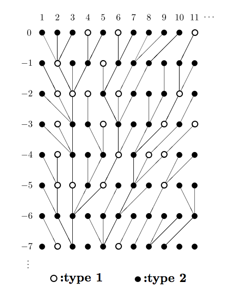
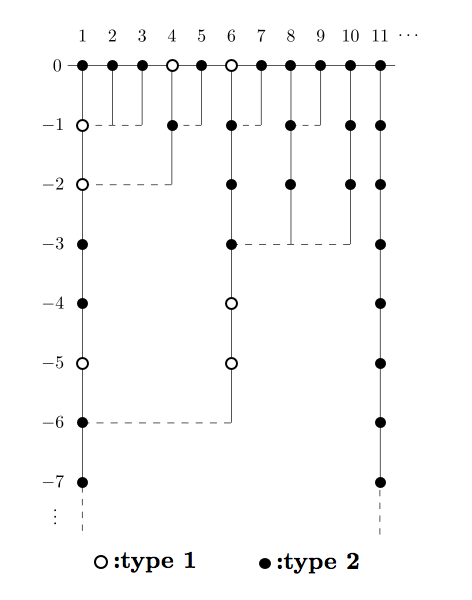
Refer to caption
Refer to caption
Figure 2: Planar embedding of a two-type branching process (left), and the types along the ancestral lineages 𝑨i\bm{A}_{i} (right)

The auxiliary process also needs to be enriched to contain information on types. We define the process (𝑫i)i≥1(\bm{D}_{i})_{i\geq 1} of vector valued sequences 𝑫i={𝑫i​(n),n≥1}\bm{D}_{i}=\{\bm{D}_{i}(n),n\geq 1\} in such a way that each 𝑫i​(n)∈{1,2​…,k}ℕ\bm{D}_{i}(n)\in\{1,2\ldots,k\}^{\mathbb{N}} is a vector of types of offspring of the ancestor ai​(n)a_{i}(n) in generation −n-n embedded to the right of the lineage of (0,i)(0,i) that are ‘survivors’ (meaning that they have progeny that are alive in generation 00):

𝑫i​(n)\displaystyle\bm{D}_{i}(n)\!\!\!\! :=vector of types of surviving offspring of individual ​(−n,ai​(n))​ in generation −n\displaystyle:=\mbox{vector of {\it types} of {\it surviving} offspring of individual }(-n,a_{i}(n))\mbox{ in generation }-n
embedded in the ancestral tree to the right of and including the lineage of ​(0,i)\displaystyle\mbox{ embedded in the {\it ancestral tree} to the right of and {\it including} the lineage of }(0,i)

Clearly ‖𝑫i​(n)‖≥1\|\bm{D}_{i}(n)\|\geq 1, and note that Di​(n):=‖𝑫i​(n)‖−1D_{i}(n):=\|\bm{D}_{i}(n)\|-1 is the number of surviving offspring of individual (−n,ai​(n))(-n,a_{i}(n)) embedded to the right of (and excluding) the lineage of (0,i)(0,i), as in the single type process.

In order to describe the law of 𝑫\bm{D} we need to provide notation for surviving lineages. Let 𝝃ℓ\bm{\xi}_{\ell} be the offspring distribution of an individual of type ℓ\ell with probability generating function fℓ​(𝒔)f_{\ell}(\bm{s}). For individual (n,i)(n,i) the law of the number of its offspring, given that its type is t⁡(n,i)=ℓ\mathrm{t}(n,i)=\ell, is that of 𝝃ℓ\bm{\xi}_{\ell}. The survival probability of an offspring of some type ℓ′\ell^{\prime} in some generation −n′-n^{\prime} is given by pn′−1,ℓ′:=1−fℓ′(n′−1)​(0,0,…,0)p_{n^{\prime}-1,\ell^{\prime}}:=1-f_{\ell^{\prime}}^{(n^{\prime}-1)}(0,0,\ldots,0) where fℓ′(n′−1)f_{\ell^{\prime}}^{(n^{\prime}-1)} is the (n′−1)(n^{\prime}-1)-fold composition of ff.

We consider all the survivor progeny of a generation −n-n ancestor of some individual from the standing population, and suppose that the type of this generation −n-n ancestor is ℓ\ell. For different ℓ′∈{1,…,k}\ell^{\prime}\in\{1,\ldots,k\} let {ϵn,ℓ′1,ϵn,ℓ′2,…}\{\epsilon^{1}_{n,\ell^{\prime}},\epsilon^{2}_{n,\ell^{\prime}},\ldots\} be independent sequences of i.i.d. Bernoulli variables with parameters ℙ⁡(ϵn,ℓ′m=1)=pn−1,ℓ′\mathbb{P}(\epsilon^{m}_{n,\ell^{\prime}}=1)=p_{n-1,\ell^{\prime}}. Start with an independent variable 𝝃ℓ\bm{\xi}_{\ell}, which takes values in ℕ0k\mathbb{N}_{0}^{k} and has 𝝃ℓ,ℓ′\bm{\xi}_{\ell,\ell^{\prime}} offspring of type ℓ′\ell^{\prime}, and define the vector of random sums:

𝜻n,ℓ:=(∑m=1𝝃ℓ,1ϵn,1m,…,∑m=1𝝃ℓ,kϵn,km)\bm{\zeta}_{n,\ell}:=\big(\sum_{m=1}^{\bm{\xi}_{\ell,1}}\epsilon^{m}_{n,1},\ldots,\sum_{m=1}^{\bm{\xi}_{\ell,k}}\epsilon^{m}_{n,k}\big)

whose ℓ′\ell^{\prime} coordinate is denoted by 𝜻n,ℓ,ℓ′\bm{\zeta}_{n,\ell,\ell^{\prime}}. Then, the law of 𝜻n,ℓ′\bm{\zeta}^{\prime}_{n,\ell}, which represents the number of surviving offspring of different types in generation −(n−1)-(n-1) of the initiating generation −n-n ancestor, is given by:

𝜻n,ℓ′:=d(𝜻n,ℓ|∑ℓ′=1k𝜻n,ℓ,ℓ′≠0).\bm{\zeta}^{\prime}_{n,\ell}:\mathop{=}^{d}(\bm{\zeta}_{n,\ell}\big|\sum_{\ell^{\prime}=1}^{k}\bm{\zeta}_{n,\ell,\ell^{\prime}}\neq 0).

Let 𝒅⁡(𝜻n,ℓ′)∈{1,2,…,k}ℕ\bm{d}(\bm{\zeta}^{\prime}_{n,\ell})\in\{1,2,\ldots,k\}^{\mathbb{N}} be an ordering of all the offspring counted by 𝜻n,ℓ′\bm{\zeta}^{\prime}_{n,\ell} chosen uniformly at random from all possible orderings (or in some specific way, as in the next section).

Recall that 𝒗[j]\bm{v}_{[j]} denotes the jj-th coordinate of a vector 𝒗∈{1,2​…,k}ℕ\bm{v}\in\{1,2\ldots,k\}^{\mathbb{N}}. Then ȷ:=𝒅​(𝜻n,ℓ′)[1]\jmath:=\bm{d}(\bm{\zeta}^{\prime}_{n,\ell})_{[1]} is the type of the left most surviving offspring in generation −(n−1)-(n-1) of the ancestor from generation −n-n. Again, for different ℓ′∈{1,…,k}\ell^{\prime}\in\{1,\ldots,k\} let {ϵn−1,ℓ′1,ϵn−1,ℓ′2,…}\{\epsilon^{1}_{n-1,\ell^{\prime}},\epsilon^{2}_{n-1,\ell^{\prime}},\ldots\} be independent sequences of i.i.d. Bernoulli variables with parameters ℙ⁡(ϵn−1,ℓ′m=1)=pn−2,ℓ′\mathbb{P}(\epsilon^{m}_{n-1,\ell^{\prime}}=1)=p_{n-2,\ell^{\prime}} (independent of all earlier sequences of Bernoulli variables). Proceed with an independent variable 𝝃ȷ\bm{\xi}_{\jmath}, and define the vector of random sums:

𝜻n−1,ȷ:=(∑m=1𝝃ȷ,1ϵn−1,1m,…,∑m=1𝝃ȷ,kϵn−1,km),𝜻n−1,ȷ′:=d(𝜻n−1,ȷ|∑ℓ′=1k𝜻n−1,ȷ,ℓ′≠0).\bm{\zeta}_{n-1,\jmath}:=\big(\sum_{m=1}^{\bm{\xi}_{\jmath,1}}\epsilon^{m}_{n-1,1},\ldots,\sum_{m=1}^{\bm{\xi}_{\jmath,k}}\epsilon^{m}_{n-1,k}\big),\quad\bm{\zeta}^{\prime}_{n-1,\jmath}:\mathop{=}^{d}(\bm{\zeta}_{n-1,\jmath}\big|\sum_{\ell^{\prime}=1}^{k}\bm{\zeta}_{n-1,\jmath,\ell^{\prime}}\neq 0).

and let 𝒅⁡(𝜻n−1,ȷ′)∈{1,2,…,k}ℕ\bm{d}(\bm{\zeta}^{\prime}_{n-1,\jmath})\in\{1,2,\ldots,k\}^{\mathbb{N}} the ordering of these surviving offspring. Then κ:=𝒅​(𝜻n−1,ȷ′)[1]\kappa:=\bm{d}(\bm{\zeta}^{\prime}_{n-1,\jmath})_{[1]} is the type of the left most surviving progeny in generation −(n−2)-(n-2) of the initiating individual from generation −n-n.

We proceed in this way recursively until generation −1-1 when we obtain the set of offspring 𝒅⁡(𝜻1,ı′)\bm{d}(\bm{\zeta}^{\prime}_{1,\imath}). In order to collect all types of the left most surviving progeny (and their siblings) in different generations 0,−1,…,−(n−2)0,-1,\ldots,-(n-2), and −(n−1)-(n-1) in one vector, we define an nn long sequence of vectors in type space initiated by individual of type ℓ\ell:

𝜼n,ℓ:=(𝒅⁡(𝜻1,ı′),…,𝒅⁡(𝜻n−2,κ′),𝒅⁡(𝜻n−1,ȷ′),𝒅⁡(𝜻n,ℓ′))\bm{\eta}_{n,\ell}:=\big(\bm{d}(\bm{\zeta}^{\prime}_{1,\imath}),\ldots,\bm{d}(\bm{\zeta}^{\prime}_{n-2,\kappa}),\bm{d}(\bm{\zeta}^{\prime}_{n-1,\jmath}),\bm{d}(\bm{\zeta}^{\prime}_{n,\ell})\big)

whose coordinates are then the vectors of surviving offspring types in different generations 𝜼n,ℓ​(1)=𝒅⁡(𝜻1,ı′)\bm{\eta}_{n,\ell}(1)=\bm{d}(\bm{\zeta}^{\prime}_{1,\imath}), … , 𝜼n,ℓ​(n−1)=𝒅⁡(𝜻n−1,ȷ′)\bm{\eta}_{n,\ell}(n-1)=\bm{d}(\bm{\zeta}^{\prime}_{n-1,\jmath}), 𝜼n,ℓ​(n):=𝒅⁡(𝜻n,ℓ′)\bm{\eta}_{n,\ell}(n):=\bm{d}(\bm{\zeta}^{\prime}_{n,\ell}).

Refer to caption
Figure 3: Collection of offspring on the ancestral lineage of individual (0,6)(0,6) originating from its common ancestor in generation −6-6 with individual (0,5)(0,5) (surviving marked with dark edges; non-surviving marked with light edges).

We introduce one final piece of notation. For a vector 𝒗∈{1,2​…,k}ℕ\bm{v}\in\{1,2\ldots,k\}^{\mathbb{N}}, let (𝒗[2],𝒗[3],…)(\bm{v}_{[2]},\bm{v}_{[3]},\ldots) define a vector obtained from 𝒗\bm{v} by eliminating the first coordinate 𝒗[1]\bm{v}_{[1]} and shifting the rest of its coordinates one coordinate to the left. Having defined the random variables 𝜼n,ℓ\bm{\eta}_{n,\ell}, for arbitrary nn and ℓ\ell, the reconstruction of the ancestral tree from the auxiliary process is possible as in the single type case.

Refer to caption
Figure 4: Sequences (Di​(⋅))i≥1(D_{i}(\cdot))_{i\geq 1} of surviving offspring types along the lineages of individuals ((,,,))i≥1((0,i))_{i\geq 1} corresponding to the ancestral tree given in Figure 2.
Theorem 2.1

The coalescent times (Ai)i≥1(A_{i})_{i\geq 1} and types along the ancestral tree (𝐀i)i≥1(\bm{A}_{i})_{i\geq 1} are both functionals of (𝐃i)i≥1(\bm{D}_{i})_{i\geq 1} given by

Ai=min⁡{n≥1:‖𝑫i​(n)‖−1≠0},𝑨i=(𝑫i+1​(1)[1],…,𝑫i+1​(Ai)[1]).A_{i}=\min\{n\geq 1:\|\bm{D}_{i}(n)\|-1\neq 0\},\quad\bm{A}_{i}=\big(\bm{D}_{i+1}(1)_{[1]},\ldots,\bm{D}_{i+1}(A_{i})_{[1]}\big).

The sequence (𝐃i)i≥1(\bm{D}_{i})_{i\geq 1} is a Markov chain with transition probabilities given by:

(𝑫i+1​(n)|𝑫i​(⋅))​=d{𝑫i​(n)for n>Ai,(𝑫i​(n)[2],𝑫i​(n)[3],…)for n=Ai,𝜼Ai−1,𝑫i​(Ai)[2](n)for 1≤n<Ai\displaystyle(\bm{D}_{i+1}(n)\,|\,\bm{D}_{i}(\cdot))\mathop{=}^{d}\left\{\begin{array}[]{lll}\bm{D}_{i}(n)&\mbox{\rm for }&n>A_{i},\\ \!\!({\bm{D}}_{i}(n)_{[2]},{\bm{D}}_{i}(n)_{[3]},\dots)&\mbox{\rm for }&n=A_{i},\\ \bm{\eta}_{{}_{A_{i}-1,\bm{D}_{i}(A_{i})_{[2]}}}(n)&\mbox{\rm for }&1\leq n<A_{i}\end{array}\right.

where the law of the Ai−1A_{i}-1 long sequence of type vectors (𝐃i+1​(1),…,𝐃i+1​(Ai−1))(\bm{D}_{i+1}(1),\ldots,\bm{D}_{i+1}(A_{i}-1)) is distributed as the vector 𝛈n,ℓ\bm{\eta}_{n,\ell} of types of the left most surviving progeny (and their siblings) in generations −1,…,−(Ai−1)-1,\ldots,-(A_{i}-1) of generation −n=−(Ai−1)-n=-(A_{i}-1) individual whose type is ℓ=𝐃i​(Ai)[2]\ell=\bm{D}_{i}(A_{i})_{[2]}.

Proof written 5.1 □\Box

The Markov chain (𝑫i)i≥1(\bm{D}_{i})_{i\geq 1} allows us to calculate some statistical features of the ancestral tree. The most relevant are coalescence times (Ai)i≥1(A_{i})_{i\geq 1} which indicate the shape of the ancestral tree, and form a non-Markovian process. We next give an explicit formula for the joint law of a coalescent time A1A_{1} of individuals (0,1)(0,1) and (0,2)(0,2) together with the values of types along the whole ancestral lineage 𝑨0=(t⁡(0,a1​(0)),t⁡(−1,a1​(1)),…)\bm{A}_{0}=(\mathrm{t}(0,a_{1}(0)),\mathrm{t}(-1,a_{1}(1)),\ldots) of individual (0,1)(0,1). It illustrates the role of ancestral types when determining branching times in the ancestral tree of the standing population. For a sequence 𝒂∈{1,…,k}ℕ0\bm{a}\in\{1,\dots,k\}^{\mathbb{N}_{0}} let 𝒂|n′\bm{a}_{|n^{\prime}} denote the vector of the first coordinates up to n′n^{\prime}-th one in this sequence 𝒂|n′:=(𝒂[0],𝒂[1],…,𝒂[n′])\bm{a}_{|n^{\prime}}:=(\bm{a}_{[0]},\bm{a}_{[1]},\dots,\bm{a}_{[n^{\prime}]}).

Proposition 2.2

For a sequence of types 𝐚=(𝐚[0],𝐚[1],…)∈{1,…,k}ℕ0\bm{a}=(\bm{a}_{[0]},\bm{a}_{[1]},\ldots)\in\{1,\ldots,k\}^{\mathbb{N}_{0}}

ℙ(A1>n,𝑨0|n−1=𝒂|n−1|𝑨0​[n]=𝒂[n])=1pn,𝒂[n]∏n′=1n(∂f𝒂[n′]​(𝒔)∂s𝒂[n′−1]|𝒔=𝟏−𝒑n′−1)\displaystyle\mathbb{P}(A_{1}>n,\bm{A}_{0|n-1}=\bm{a}_{|n-1}|\,\bm{A}_{0[n]}=\bm{a}_{[n]})=\frac{1}{p_{n,\bm{a}_{[n]}}}\prod_{n^{\prime}=1}^{n}\Bigg(\frac{\partial f_{\bm{a}_{[n^{\prime}]}}(\bm{s})}{\partial s_{\bm{a}_{[n^{\prime}-1]}}}\Big|_{\bm{s}=\bm{1}-\bm{p}_{n^{\prime}-1}}\Bigg) (5)

where 𝟏−𝐩n′−1:=(1−pn′−1,1,…,1−pn′−1,k)=𝐟(n′−1)​(𝟎)\bm{1}-\bm{p}_{n^{\prime}-1}:=(1-p_{n^{\prime}-1,1},\ldots,1-p_{n^{\prime}-1,k})=\bm{f}^{(n^{\prime}-1)}(\bm{0}) is the vector of extinction probabilities by generation n′−1n^{\prime}-1.

Proof written 5.1 □\Box

An easy modification of the formula above gives ℙ(A1=n,𝑨0|n−1=𝒂|n−1|𝑨0​[n]=𝒂[n])\mathbb{P}(A_{1}=n,\bm{A}_{0|n-1}=\bm{a}_{|n-1}|\,\bm{A}_{0[n]}=\bm{a}_{[n]}). We also have the following result on the law of the coalescent time A1A_{1}.

Corollary 2.3

For a single type value 𝐚[n]∈{1,…,k}\bm{a}_{[n]}\in\{1,\ldots,k\} and a multi-type branching process 𝐙\bm{Z}

ℙ⁡(A1>n|𝑨0​[n]=𝒂[n])=ℙ⁡(∑ℓ=1kZℓ(n)=1|𝒁(n)≠𝟎,𝒁(0)=𝒆𝒂[n]).\displaystyle\mathbb{P}(A_{1}>n|\,\bm{A}_{0[n]}=\bm{a}_{[n]})=\mathbb{P}\Big(\sum_{\ell=1}^{k}Z^{(n)}_{\ell}=1\,|\,\bm{Z}^{(n)}\neq\bm{0},\bm{Z}^{(0)}=\bm{e}_{\bm{a}_{[n]}}\Big). (6)

Proof written 5.1 □\Box

Remark 2.4

In terms of applications the joint law of A1A_{1} and 𝐀0|n−1\bm{A}_{0|n-1} is more useful for reconstructing ancestral trees. Note that the choice of embedding the offspring of each parent uniformly at random in the tree is reflected in these formulae at all. This is in particular evident in (6). Moreover, (6) can be obtained from (5) by summing over all the possible values of 𝐀0​[n′]\bm{A}_{0[n^{\prime}]} of types of the 0≤n′<n0\leq n^{\prime}<n generations’ ancestors of the individual (0,1)(0,1) which start with 𝐀0​[n]=𝐚[n]\bm{A}_{0[n]}=\bm{a}_{[n]}. In the next section we consider a different choice of ordering the offspring for a specific offspring distribution, and show consistency of these two expressions.

The statistical feature which indicates the distribution of types in the ancestral tree are coalescence times between individuals in the standing population that are of the same type. Suppose the type of the first individual in generation 00 is 𝑨0​[0]=ℓ\bm{A}_{0[0]}=\ell, and define the sequence iℓ,0:=0,iℓ,1:=min{i′>0:𝑨i′​[0]=ℓ},…,iℓ,i:=min{i′>iℓ,i−1:𝑨i′​[0]=ℓ},…\mathrm{i}_{\ell,0}:=0,\;\mathrm{i}_{\ell,1}:=\min\{i^{\prime}>0:\bm{A}_{i^{\prime}[0]}=\ell\},\;\ldots,\;\mathrm{i}_{\ell,i}:=\min\{i^{\prime}>\mathrm{i}_{\ell,i-1}:\bm{A}_{i^{\prime}[0]}=\ell\},\ldots representing the indices of consecutive individuals of type ℓ\ell from the standing population. Define the sequence of same-type coalescence times for individuals of type ℓ\ell by

Bℓ,1:=max⁡{Aiℓ,1,…,Aiℓ,2−1},…,Bℓ,i:=max⁡{Aiℓ,i,…,Aiℓ,i+1−1},…B_{\ell,1}:=\max\{A_{\mathrm{i}_{\ell,1}},\ldots,A_{\mathrm{i}_{\ell,2}-1}\},\;\ldots\;,B_{\ell,i}:=\max\{A_{\mathrm{i}_{\ell,i}},\ldots,A_{\mathrm{i}_{\ell,i+1}-1}\},\ldots

Using the values of types on the left most infinite spine 𝑨0\bm{A}_{0} we can determine the joint distribution of B𝑨0​[0],1B_{\bm{A}_{0[0]},1} and 𝑨0|n−1\bm{A}_{0|n-1} as follows.

Proposition 2.5

For a sequence of types 𝐚=(𝐚[0],𝐚[1],…)∈{1,…,k}ℕ\bm{a}=(\bm{a}_{[0]},\bm{a}_{[1]},\ldots)\in\{1,\ldots,k\}^{\mathbb{N}} with 𝐚[0]=ℓ\bm{a}_{[0]}=\ell

ℙ(Bℓ,1>n,𝑨0|n−1=𝒂|n−1|𝑨0​[n]=𝒂[n],𝑨0​[0]=ℓ)=1p(n,ℓ),𝒂[n−1]∏n′=1n(∂f𝒂[n′]​(𝒔)∂s𝒂[n′−1]|𝒔=𝟏−𝒑(n′−1,ℓ′))\displaystyle\mathbb{P}(B_{\ell,1}>n,\bm{A}_{0{|n-1}}=\bm{a}_{|n-1}|\,\bm{A}_{0[n]}=\bm{a}_{[n]},\bm{A}_{0[0]}=\ell)=\frac{1}{p_{(n,\ell),\bm{a}_{[n-1]}}}\!\!\prod_{n^{\prime}=1}^{n}\Big(\frac{\partial f_{\bm{a}_{[n^{\prime}]}}(\bm{s})}{\partial s_{\bm{a}_{[n^{\prime}-1]}}}\Big|_{\bm{s}=\bm{1}-\bm{p}_{(n^{\prime}-1,\ell^{\prime})}}\Big) (7)

where 𝟏−𝐩(n′−1,ℓ):=(1−p(n′−1.ℓ),1,…,1−p(n′−1,ℓ),k)=𝐟(n′−1)(𝐞^ℓ′)\bm{1}-\bm{p}_{(n^{\prime}-1,\ell)}:=(1-p_{(n^{\prime}-1.\ell),1},\ldots,1-p_{(n^{\prime}-1,\ell),k})=\bm{f}^{(n^{\prime}-1)}(\bm{\hat{e}}_{\ell^{\prime}}) with 𝐞^ℓ′=𝟏−𝐞ℓ′\bm{\hat{e}}_{\ell^{\prime}}=\bm{1}-\bm{e}_{\ell^{\prime}}, is the vector of extinction probabilities for lineages with type ℓ\ell descendants after n′−1n^{\prime}-1 generations.

Proof written 5.1 □\Box

As before, we also have the following result on the law of the same-type coalescent time Bℓ,1B_{\ell,1}.

Corollary 2.6

For a single type value 𝐚[n]∈{1,…,k}\bm{a}_{[n]}\in\{1,\ldots,k\} and a multi-type branching process 𝐙\bm{Z}

ℙ⁡(Bℓ,1>n|𝑨0​[n]=𝒂[n],𝑨0​[0]=ℓ)=ℙ⁡(Zℓ(n)=1|Zℓ(n)≠0,𝒁(0)=𝒆𝒂[n]).\displaystyle\mathbb{P}(B_{\ell,1}>n|\,\bm{A}_{0[n]}=\bm{a}_{[n]},\bm{A}_{0[0]}=\ell)=\mathbb{P}\big(Z^{(n)}_{\ell}=1\,|\,Z^{(n)}_{\ell}\neq 0,\bm{Z}^{(0)}=\bm{e}_{\bm{a}_{[n]}}\big). (8)

Proof written 5.1 □\Box

It might be tempting to provide a formula for the distribution of A2,A3,…A_{2},A_{3},\dots and Bℓ,2,Bℓ,3,…B_{\ell,2},B_{\ell,3},\dots in a similar vein using the values of the types on the ancestral lineage of the individuals (0,2),(0,3),…(0,2),(0,3),\ldots respectively. The information, analogous to that of types of individuals on the left most (infinite into the past) spine 𝑨0\bm{A}_{0} used in the formulae for A1A_{1} and Bℓ,1B_{\ell,1}, which one would need to use for Ai+2A_{i+2} would be the types along the ancestral lineage of (0,i+1)(0,i+1). That is, for i≥0i\geq 0 one could define the infinite ancestral lineage 𝑨i∞\bm{A}^{\infty}_{i} of individual (0,i+1)(0,i+1) as the infinite sequence:

𝑨i∞:=(t⁡(0,ai+1​(0)),t⁡(−1,ai+1​(1)),t⁡(−2,ai+1​(2)),…),\bm{A}^{\infty}_{i}:=(\mathrm{t}(0,a_{i+1}(0)),\mathrm{t}(-1,a_{i+1}(1)),\mathrm{t}(-2,a_{i+1}(2)),\ldots),

Note that the restriction of 𝑨i∞\bm{A}^{\infty}_{i} to its first AiA_{i} entries equals the sequence 𝑨i\bm{A}_{i} called the ancestral lineage of (0,i+1)(0,i+1), and that 𝑨0∞=𝑨0\bm{A}^{\infty}_{0}=\bm{A}_{0}. It is easy to see, as a consequence of Theorem 2.1, that (𝑨i∞)i≥1(\bm{A}^{\infty}_{i})_{i\geq 1} is also a functional of (𝑫i)i≥1(\bm{D}_{i})_{i\geq 1} given by:

𝑨i∞=(𝑫i+1​(1)[1],𝑫i+1​(2)[1],𝑫i+1​(3)[1],…).\bm{A}^{\infty}_{i}=(\bm{D}_{i+1}(1)_{[1]},\bm{D}_{i+1}(2)_{[1]},\bm{D}_{i+1}(3)_{[1]},\ldots).

This follows from the fact that the first 1≤n≤Ai1\leq n\leq A_{i} entries in this sequence are the same as in 𝑨i\bm{A}_{i}, while for the subsequent n>Ain>A_{i} entries the ancestry of (0,i+1)(0,i+1) is equal to the ancestry of (0,i)(0,i) (as their ancestors already coalesced) and we have 𝑫i+1​(n)=𝑫i​(n)\bm{D}_{i+1}(n)=\bm{D}_{i}(n).

Now, providing a formula for ℙ⁡(Ai+2>n|𝑨i+1​[n]=𝒂[n])\,\mathbb{P}(A_{i+2}>n|\,\bm{A}_{i+1[n]}=\bm{a}_{[n]})\, for any i≥0i\geq 0 can be done only in case the branching mechanism is such that in the coalescent point-process all points are simple (have multiplicities equal to one). This is because, in case of multiple coalescence points, all ancestral lineages, except for that of (0,1)(0,1), in addition to information about the lineage of individual (0,i)(0,i) also contains information about the ancestral lineages of (0,i′),1≤i′<i(0,i^{\prime}),1\leq\mathrm{i}^{\prime}<i. In other words, the calculation (used in the proofs of the Propositions 2.2 and 2.5, see Section 5) which exploits the equivalence {A1>n,𝑨0|n−1=𝒂|n−1}\{A_{1}>n,\bm{A}_{0|n-1}=\bm{a}_{|n-1}\} iff {individuals 𝒂[n′],1≤n′≤n\bm{a}_{[n^{\prime}]},1\leq n^{\prime}\leq n on the ancestral lineage 𝑨0\bm{A}_{0} have a single offspring with descendants surviving to generation 00} is no longer valid in general. This is a clear consequence of the fact that the process (𝑨i,i≥0)(\bm{A}_{i},i\geq 0) is itself not Markovian, unless we are in the special case for the offspring distribution which is of linear-fractional form. In the next Section we explore this special case, and extend the above results for the coalescent times as well as for the same-type coalescence times.

Remark 2.7

The construction of the ancestral tree is based on the Markovian property of the auxiliary process (𝐃i)i≥1(\bm{D}_{i})_{i\geq 1}. To initiate the process, we need to draw 𝐃1\bm{D}_{1} from 𝛈∞,ℓ∞\bm{\eta}_{\infty,\ell_{\infty}} for some (infinitely old) originating type ℓ∞\ell_{\infty}. One way to draw from this distribution would be to start from generation 00 and time reverse the quasi-stationary distribution for the branching process. For the case of a single type branching process a construction like this was discussed in [4]. The multi-type extension is straightforward, with the infinitely old originating individual having, in the ρ≤1\rho\leq 1 case, the size-biased version of the offspring distribution given by

ℙ^​(𝒁(1)=𝒛|𝒁(0)=𝒆ℓ)=ℙ⁡(𝒁(1)=𝒛|𝒁(0)=𝒆ℓ)ρ​𝒛⋅u𝒆ℓ⋅u\widehat{\mathbb{P}}(\bm{Z}^{(1)}=\bm{z}|\bm{Z}^{(0)}=\bm{e}_{\ell})=\frac{\mathbb{P}(\bm{Z}^{(1)}=\bm{z}|\bm{Z}^{(0)}=\bm{e}_{\ell})}{\rho}\frac{\bm{z}\cdot u}{\bm{e}_{\ell}\cdot u}

.

3 Special case: Linear-fractional branching processes

Many of the complications which arise in calculating the distribution of ancestral trees in multi-type branching processes simplify a great deal in the special case when the offspring distribution is of the linear-fractional (LF) type. This type of offspring distribution leads to a number of particularly nice features involving the memoryless property of the geometric distribution. We first recall the definition of the multi-type linear-fractional offspring distribution, and then give a series of specific results for the distribution of the ancestral tree of the standing population, which both illustrate and extend our general results form the previous Section.

3.1 Multi-type linear-fractional branching process

We use the same notation as [19] for ease of drawing on known results and making comparisons. Let 𝑯\bm{H} be a k×kk\times k sub-stochastic matrix, that is, each row 𝒉ℓ\bm{h}_{\ell} of 𝑯\bm{H} is a non-negative vector with ∑ℓ′=1khℓ​ℓ′≤1\sum_{\ell^{\prime}=1}^{k}h_{\ell\ell^{\prime}}\leq 1, and let hℓ​0=1−∑ℓ′=1khℓ​ℓ′h_{\ell 0}=1-\sum_{\ell^{\prime}=1}^{k}h_{\ell\ell^{\prime}}. Let 𝒈\bm{g} be a non-negative vector such that 𝒈​𝟏t=∑ℓ′=1kgℓ′=1\bm{g}\bm{1}^{\mathrm{t}}=\sum_{\ell^{\prime}=1}^{k}g_{\ell^{\prime}}=1. Let m>0m>0. For any 𝒛=(z1,…,zk)∈ℕ0k\bm{z}=(z_{1},\ldots,z_{k})\in\mathbb{N}_{0}^{k} let |𝒛|=∑ℓ=1kzℓ|\bm{z}|=\sum_{\ell=1}^{k}z_{\ell}.

A random vector 𝝃ℓ\bm{\xi}_{\ell} taking values in ℕ0k\mathbb{N}_{0}^{k} has a linear-fractional distribution LF (𝐡ℓ,𝐠,m)(\bm{h}_{\ell},\bm{g},m) if for any non-negative integer vector 𝒛=(z1,…,zk)\bm{z}=(z_{1},\ldots,z_{k})

ℙ⁡(|𝝃ℓ|=0)=hℓ​0,ℙ⁡(𝝃ℓ=𝒆ℓ′+𝒛)=hℓ​ℓ′​m|𝒛|(1+m)|𝒛|+1​(|𝒛|z1,…,zk)​𝒈𝒛,\mathbb{P}\big(|\bm{\xi}_{\ell}|=0\big)=h_{\ell 0},\quad\mathbb{P}\big(\bm{\xi}_{\ell}=\bm{e}_{\ell^{\prime}}+\bm{z}\big)=h_{\ell\ell^{\prime}}\frac{m^{|\bm{z}|}}{(1+m)^{|\bm{z}|+1}}\left(\begin{array}[]{cc}|\bm{z}|\\ z_{1},\ldots,z_{k}\end{array}\right)\bm{g}^{\bm{z}},

where 𝒈𝒛=g1z1⋯gkzk\bm{g}^{\bm{z}}=g_{1}^{z_{1}}\cdots g_{k}^{z_{k}}. The probability generating function of 𝝃ℓ\bm{\xi}_{\ell} has the linear fractional form

fℓ​(𝒔)=hℓ​0+∑ℓ′=1khℓ​ℓ′​sℓ′1+m−m​∑ℓ′=1kgℓ′​sℓ′.f_{\ell}(\bm{s})=h_{\ell 0}+\frac{\sum_{\ell^{\prime}=1}^{k}h_{\ell\ell^{\prime}}s_{\ell^{\prime}}}{1+m-m\sum_{\ell^{\prime}=1}^{k}g_{\ell^{\prime}}s_{\ell^{\prime}}}.

One can also represent the random vector 𝝃ℓ\bm{\xi}_{\ell} as a sequence of offsprings, where the first offspring has type distribution given by 𝒉ℓ\bm{h}_{\ell} and the children after the first one have geometric distribution with mean mm and type distribution given by 𝒈\bm{g} independently for each offspring. Moreover, the probability generating function of (𝝃ℓ|𝝃ℓ≠𝟎)(\bm{\xi}_{\ell}|\bm{\xi}_{\ell}\neq\bm{0}) is that of a shifted Multivariate-Geometric distribution

𝔼⁡(𝒔𝝃ℓ|𝝃ℓ≠𝟎)=(1−hℓ​0)−1​∑ℓ′=1khℓ​ℓ′​sℓ′1+m−m​∑ℓ′=1kgℓ′​sℓ′.\mathbb{E}(\bm{s}^{\bm{\xi}_{\ell}}|\bm{\xi}_{\ell}\neq\bm{0})=\frac{(1-h_{\ell 0})^{-1}\sum_{\ell^{\prime}=1}^{k}h_{\ell\ell^{\prime}}s_{\ell^{\prime}}}{1+m-m\sum_{\ell^{\prime}=1}^{k}g_{\ell^{\prime}}s_{\ell^{\prime}}}.

A multi-type linear-fractional branching process LF⁡(𝑯,𝒈,m){\rm LF}\,\!(\bm{H},\bm{g},m) is a branching process in which each individual of type ℓ∈{1,…,k}\ell\in\{1,\ldots,k\} reproduces according to the LF⁡(𝒉ℓ,𝒈,m){\rm LF}\,\!(\bm{h}_{\ell},\bm{g},m) offspring distribution 𝝃ℓ\bm{\xi}_{\ell}. In other words, the probability generating function of the offspring distribution is 𝒇⁡(𝒔)=(f1,…,fk)​(𝒔)\bm{f}(\bm{s})=(f_{1},\ldots,f_{k})(\bm{s}) with fℓf_{\ell} as above. Its mean matrix is given by 𝑴=𝑯+m​𝑯​𝟏t​𝒈\bm{M}=\bm{H}+m\bm{H}\bm{1}^{\mathrm{t}}\bm{g}.

The fact that the parameters 𝒈\bm{g} and mm do not depend on the parent’s type ensures that the population size in each generation of this process also has a linear fractional distribution. This is given by the following known result.

Theorem 3.1 (Proposition 3 [9], Theorem 3 [19])

The nn-th generation population size vector 𝐙(n)\bm{Z}^{(n)} of a multi-type linear-fractional branching process LF⁡(𝐇,𝐠,m){\rm LF}\,\!(\bm{H},\bm{g},m) started with one individual 𝐙(0)=𝐞ℓ\bm{Z}^{(0)}=\bm{e}_{\ell} has a linear-fractional distribution LF⁡(𝐡ℓ(n),𝐠(n),m(n)){\rm LF}\,\!(\bm{h}_{\ell}^{(n)},\bm{g}^{(n)},m^{(n)}) whose parameters are determined by:

m(n)\displaystyle m^{(n)}\!\!\! =\displaystyle= m​𝒈​(𝑰+𝑴+⋯+𝑴n−1)​𝟏t,\displaystyle\!\!m\bm{g}(\bm{I}+\bm{M}+\cdots+\bm{M}^{n-1})\bm{1}^{\mathrm{t}},
𝒈(n)\displaystyle\bm{g}^{(n)}\! =\displaystyle= mm(n)​𝒈​(𝑰+𝑴+⋯+𝑴n−1),\displaystyle\!\!\!\!\frac{\!\!\!m}{\,m^{(n)}}\,\bm{g}(\bm{I}+\bm{M}+\cdots+\bm{M}^{n-1}), (9)
𝑯(n)\displaystyle\bm{H}^{(n)}\!\!\! =\displaystyle= 𝑴n−m(n)1+m(n)​𝑴n​𝟏t​𝒈(n),\displaystyle\!\!\bm{M}^{n}-\frac{m^{(n)}}{1+m^{(n)}}\bm{M}^{n}\bm{1}^{t}\bm{g}^{(n)},

where the vector 𝐡ℓ(n)\bm{h}_{\ell}^{(n)} is the ℓ\ell-th row of the matrix 𝐇(n)\bm{H}^{(n)}, and 𝟏t\bm{1}^{\mathrm{t}} is the transpose of 𝟏=(1,…,1)\bm{1}=(1,\ldots,1).

Note that, as a consequence, (𝒁(n)|𝒁(n)≠𝟎,𝒁(0)=𝒆ℓ)(\bm{Z}^{(n)}|\bm{Z}^{(n)}\neq\bm{0},\bm{Z}^{(0)}=\bm{e}_{\ell}) is distributed as a shifted Multivariate-Geometric distribution

𝔼⁡(𝒔Z(n)|𝒁(n)≠𝟎,𝒁(0)=𝒆ℓ)=(1−hℓ​0(n))−1​∑ℓ′=1khℓ​ℓ′(n)​sℓ′1+m(n)−m(n)​∑ℓ′=1kgℓ′(n)​sℓ′.\mathbb{E}(\bm{s}^{Z^{(n)}}|\bm{Z}^{(n)}\neq\bm{0},\bm{Z}^{(0)}=\bm{e}_{\ell})=\frac{(1-h_{\ell 0}^{(n)})^{-1}\sum_{\ell^{\prime}=1}^{k}h_{\ell\ell^{\prime}}^{(n)}s_{\ell^{\prime}}}{1+m^{(n)}-m^{(n)}\sum_{\ell^{\prime}=1}^{k}g_{\ell^{\prime}}^{(n)}s_{\ell^{\prime}}}.

This theorem was proved in [9] using an algebraic approach, while [19] provided a different proof using the jumping contour representation of the branching process and its nice Markovian structure. As shown in [19] this result and the linear-fractional definition also apply for the case of infinitely many types. See [19] also for a discussion about the use of linear-fractional branching processes in applications.

3.2 Coalescent times in linear-fractional ancestral tree

We use the coalescent point-process construction to get simpler results for the distribution of coalescent times (and same-type coalescent times) for this special class of multi-type branching processes. For this purpose we make one change in our original construction pertaining to the embedding of the multi-type tree in the plane. For a general offspring distribution we made the assumption that the offspring of any parent are embedded in a left to right order chosen uniformly at random from all possible orderings. For the linear-fractional offspring distribution we make a particular assumption that the offspring with distribution given by the vector 𝒉⋅\bm{h}_{\cdot} is embedded as the left most individual, followed by the rest of the offspring according to an arbitrary order.

Proposition 3.2

The coalescence times (Ai)i≥0(A_{i})_{i\geq 0} in the ancestral tree of a LF⁡(𝐇,𝐠,m){\rm LF}\,\!(\bm{H},\bm{g},m) branching process are independent identically distributed variables with

P⁡(A1>n)=∏n′=1n11+m−m​∑ℓ′=1k𝒈ℓ′​hℓ′​0(n′−1)=11+m(n),P(A_{1}>n)=\prod_{n^{\prime}=1}^{n}\frac{1}{1+m-m\sum_{\ell^{\prime}=1}^{k}\bm{g}_{\ell^{\prime}}h_{\ell^{\prime}0}^{(n^{\prime}-1)}}=\frac{1}{1+m^{(n)}}, (10)

where hℓ′​0(n′−1)=1−𝐡ℓ′(n′−1)​𝟏th_{\ell^{\prime}0}^{(n^{\prime}-1)}\!\!=1-\bm{h}_{\ell^{\prime}}^{(n^{\prime}-1)}\bm{1}^{\mathrm{t}}, 𝐡ℓ′(n′−1)\bm{h}_{\ell^{\prime}}^{(n^{\prime}-1)}\!\! is the ℓ′\ell^{\prime}-th row of the matrix 𝐇(n)\bm{H}^{(n)} from (9), hℓ′​0(0)=0​∀ℓ′h^{(0)}_{\ell^{\prime}0}=0\;\forall\ell^{\prime}. The law of the coalescent times also satisfies ℙ⁡(A1>n|𝐀0​[n]=𝐚[n])=ℙ⁡(A1>n)\mathbb{P}\big(A_{1}>n|\,\bm{A}_{0[n]}=\bm{a}_{[n]}\big)=\mathbb{P}(A_{1}>n).

Proof written 5.2 □\Box

Remark 3.3

The second, simpler expression in (10) can be obtained either using arithmetic properties of parameters (9) from Theorem 3.1, or using the expression in terms of the nn-th generation of a multi-type LF branching process.

Proposition 3.4

For any type ℓ∈{1,…,k}\ell\in\{1,\dots,k\}, the same-type coalescence times (Bℓ,i)i≥0(B_{\ell,i})_{i\geq 0} are independent identically distributed variables with

P⁡(Bℓ,1>n|𝑨0​[0]=ℓ)=∏n′=1n11+m−m​∑ℓ′=1k𝒈ℓ′​h~ℓ′​0(n′−1)=11+m(n)​gℓ(n)P(B_{\ell,1}>n|\,\bm{A}_{0[0]}=\ell)=\prod_{n^{\prime}=1}^{n}\frac{1}{1+m-m\sum_{\ell^{\prime}=1}^{k}\bm{g}_{\ell^{\prime}}\tilde{h}_{\ell^{\prime}0}^{(n^{\prime}-1)}}=\frac{1}{1+m^{(n)}g^{(n)}_{\ell}} (11)

where, for n′>1n^{\prime}>1, 𝐡~ℓ′​0(n′−1)\tilde{\bm{h}}_{\ell^{\prime}0}^{(n^{\prime}-1)} is given in terms of hℓ′​0(n′−1)=1−𝐡ℓ′(n′−1)​𝟏th_{\ell^{\prime}0}^{(n^{\prime}-1)}=1-\bm{h}_{\ell^{\prime}}^{(n^{\prime}-1)}\bm{1}^{\mathrm{t}} and parameters in (9) by

h~ℓ′​0(n′−1)=hℓ′​0(n′−1)+1−hℓ′​0(n′−1)−hℓ′​ℓ(n′−1)1+m(n′−1)​gℓ(n′−1),\tilde{h}_{\ell^{\prime}0}^{(n^{\prime}-1)}=h^{(n^{\prime}-1)}_{\ell^{\prime}0}+\frac{1-h^{(n^{\prime}-1)}_{\ell^{\prime}0}-h^{(n^{\prime}-1)}_{\ell^{\prime}\ell}}{1+m^{(n^{\prime}-1)}g^{(n^{\prime}-1)}_{\ell}},

and h~ℓ′​0(0)=1​∀ℓ′≠ℓ\tilde{h}_{\ell^{\prime}0}^{(0)}=1\;\forall\ell^{\prime}\neq\ell, while h~ℓ​0(0)=0\tilde{h}_{\ell 0}^{(0)}=0.

Proof written 5.2 □\Box

Although the multi-type LF offspring distribution has a seemingly small level of dependence between the offspring and parent type, it still affects the distribution of types in the ancestral tree. One can also consider a multi-type branching process where offspring distribution is completely independent of the parent type. In this case the shape of the tree and the types on the tree can be decoupled, and the distribution of types is only governed by the frequency of this type in the population.

Consider a special case of a LF distribution where 𝑯:=𝟏t​𝒉\bm{H}:=\bm{1}^{\mathrm{t}}\bm{h}, for 𝒉​𝟏t=h1+⋯+hk≤1\bm{h}\bm{1}^{\mathrm{t}}=h_{1}+\cdots+h_{k}\leq 1, then each parent has the same LF⁡(𝒉,𝒈,m){\rm LF}\,\!(\bm{h},\bm{g},m) offspring distribution. Further, if we are to have no distinction between the first offspring and the rest, then consider 𝒉:=(1−h0)​𝒈\bm{h}:=(1-h_{0})\bm{g}, for h0∈(0,1)h_{0}\in(0,1). In this case all parents have the same offspring laws where their number of offspring has a single-type LF(h0,m)(h_{0},m) distribution with probability generating function h0+(1−h0)​s/(1+m−m​s)h_{0}+(1-h_{0})s/(1+m-ms), given the number of their offspring, the distribution of types for these offspring is Multinomial with parameter 𝒈\bm{g}. In this case we get the following formulae for the law of coalescence times and same-type coalescence times.

Corollary 3.5

If the offspring distribution of each parent is independent of the parent’s type with LF⁡((1−h0)​𝟏t​𝐠,𝐠,m){\rm LF}\,\!((1-h_{0})\bm{1}^{\mathrm{t}}\bm{g},\bm{g},m) distribution, then

ℙ⁡(A1>n)\displaystyle\mathbb{P}(A_{1}>n) =\displaystyle= {m−h0​(1+m)m​(1+m)n​(1−h0)n−h0​(1+m)if(1−h0)(1+m)≠11−h01−h0+n​h0if(1−h0)(1+m)=1\displaystyle\Bigg\{\begin{tabular}[]{ll}$\frac{m-h_{0}(1+m)}{m(1+m)^{n}(1-h_{0})^{n}-h_{0}(1+m)}$&$\mathrm{if}$\; $(1-h_{0})(1+m)\neq 1$\\ $$\\ $\frac{1-h_{0}}{1-h_{0}+nh_{0}}$&$\mathrm{if}$\; $(1-h_{0})(1+m)=1$\end{tabular}

and

ℙ⁡(Bℓ,1>n|𝑨0​[0]=ℓ)=1−ℙ⁡(A1≤n)1−ℙ⁡(A1≤n)​(1−gℓ)\displaystyle\mathbb{P}(B_{\ell,1}>n|\,\bm{A}_{0[0]}=\ell)=\frac{1-\mathbb{P}(A_{1}\leq n)}{1-\mathbb{P}(A_{1}\leq n)(1-g_{\ell})} (13)

Proof written - 5.2□\Box

As expected, the distribution of types 𝒈\bm{g} has no effect on the law of (Ai)i≥1(A_{i})_{i\geq 1} and the shape of the tree, but appears in the distribution of types in the tree as indicated by the law of (Bℓ,i)i≥1(B_{\ell,i})_{i\geq 1}.

We can consider the process of coalescent times (Ai)i≥0(A_{i})_{i\geq 0} as a simple point-process AA on {1,2,…}×{−1,−2,…}\{1,2,\dots\}\times\{-1,-2,\dots\} with intensity measure νA​[{i}×{−(n+1),…}]=ℙ⁡(A1>n)\nu_{A}\big[\{i\}\times\{-(n+1),\dots\}\big]=\mathbb{P}(A_{1}>n), ∀i≥1\forall i\geq 1. Similarly for each ℓ∈{1,…,k}\ell\in\{1,\dots,k\}, (Bℓ,i)i≥0(B_{\ell,i})_{i\geq 0} can be regarded as a simple point-process BℓB_{\ell} with intensity νBℓ​[{i}×{−(n+1),…}]=ℙ⁡(Bℓ,1>n)\nu_{B_{\ell}}\big[\{i\}\times\{-(n+1),\dots\}\big]=\mathbb{P}(B_{\ell,1}>n) on {1,2,…}×{−1,−2,…}\{1,2,\dots\}\times\{-1,-2,\dots\}. Note that for any i≥1i\geq 1, n≥1n\geq 1 (13) implies that

νBℓ​[{i}×{−1,…,−n}]=νA​[{i}×{−1,…,−n}]​gℓνA​[{i}×{−(n+1),…}]+νA​[{i}×{−1,…,−n}]​gℓ\nu_{B_{\ell}}\big[\{i\}\times\{-1,\dots,-n\}\big]=\frac{\nu_{A}\big[\{i\}\times\{-1,\dots,-n\}\big]g_{\ell}}{\nu_{A}\big[\{i\}\times\{-(n+1),\dots\}\big]+\nu_{A}\big[\{i\}\times\{-1,\dots,-n\}\big]g_{\ell}}

showing that only a fraction of all coalescent times are candidates for same-type coalescence times for type ℓ\ell. Intuitively, when considering Bℓ,iB_{\ell,i} mark each coalescent time Ai,Ai+1,…A_{i},A_{i+1},\dots with the probability that the next individual in the standing population is of type ℓ\ell, which is gℓg_{\ell}. Then, from the filtered view of Bℓ,iB_{\ell,i}, a coalescence time Ai,Ai+1,…A_{i},A_{i+1},\dots either occurs outside the set {1,…,n}\{1,\dots,n\}, or it occurs inside this set and it links to a standing individual of type ℓ\ell.

Note that the intensity measures {νBℓ}ℓ∈{1,…,k}\{\nu_{B_{\ell}}\}_{\ell\in\{1,\dots,k\}} do not partition in full the measure νA\nu_{A}, since for any n≥1n\geq 1 such that ℙ⁡(Ai>n)>0\mathbb{P}(A_{i}>n)>0 we have that

∑ℓ=1kνBℓ​[{i}×{−1,…,−n}]<∑ℓ=1kνA​[{i}×{−1,…,−n}]​gℓ=νA​[{i}×{−1,…,−n}].\sum_{\ell=1}^{k}\nu_{B_{\ell}}\big[\{i\}\times\{-1,\dots,-n\}\big]<\sum_{\ell=1}^{k}{\nu_{A}\big[\{i\}\times\{-1,\dots,-n\}\big]g_{\ell}}={\nu_{A}\big[\{i\}\times\{-1,\dots,-n\}\big]}.

This is a consequence of the fact that not all coalescence times are in fact same-type coalescence times for some ℓ\ell (for example, in Figure 2 the coalescence time A4=1A_{4}=1 of (0,4)(0,4) and (0,5)(0,5) is neither a same-type 𝟏\bm{1} nor a a same-type 𝟐\bm{2} coalescence time).

3.3 Comparison of ancestral trees in two-type models

We next give an example of using the same-type coalescent times to investigate the effect of differences in offspring distribution on the distribution of types in the ancestral trees they produce. One question that motivated our work is the effect of different diversification rates for different types of individuals (phenotypes). We translate these questions into a discrete time defining an asymmetrical offspring distribution law.

Specifically, in a population with only two types of individuals, if the transition rates of one type to the other are relatively high, while the other type never transitions into the first, this will be reflected in the distribution of types along the tree. In a discrete time process this is translated in the probability of a parent of the first type giving birth to individuals of the second type and vice versa. We consider this difference in the context of a two-type LF offspring distribution. In order to investigate only the effect on the distribution of types, we will make the distribution of the shape of the tree the same in both cases.

We consider the following two LF offspring distributions on k=2k=2 types of individuals. Let the parameters 𝒈=(g,1−g),g∈[0,1/2]\bm{g}=(g,1-g),g\in[0,1/2], m>0m>0 and h1=1−h0,h0∈[0,1]h_{1}=1-h_{0},h_{0}\in[0,1]\; be the same in both distributions, and for p∈(0,1)p\in(0,1) let

𝑯𝐬=h1​(p1−p1−pp),𝑯𝐚=h1​(p1−p01),\bm{H}_{\mathbf{s}}=h_{1}\left(\begin{array}[]{cc}p&1-p\\ 1-p&p\end{array}\right),\quad\bm{H}_{\mathbf{a}}=h_{1}\left(\begin{array}[]{cc}p&1-p\\ 0&1\end{array}\right),

be, respectively, associated with the symmetrical and the asymmetrical offspring distribution. In the symmetrical case parents of either type produce offspring of their own type and of the other type. In the asymmetrical case only a parent of type 𝟏\bm{1} will do that, while a parent of type 𝟐\bm{2} can only produce offspring of its own type. Since the number of offspring of each parent depends only on h0h_{0} and mm, the distribution of the ancestral tree with types erased will be the same in both cases. However, the distribution of the two types 𝟏\bm{1} and 𝟐\bm{2} are different, as can be seen in the following result.

Remark 3.6

Note that we can assume without loss of generality that g∈[0,1/2]g\in[0,1/2], since in case g∈[1/2,1]g\in[1/2,1] we can simply reverse the notation of the two types. For p=1p=1 there is no asymmetry, nor are there offspring of different type than the parent - individuals in the whole tree are all of the same type. For (g,p)=(1/2,1/2)(g,p)=(1/2,1/2) the symmetric case is special, and the offspring distribution is independent of the type of the parent, as discussed in Corollary 3.5.

Proposition 3.7

The distributions of coalescence times (Ai)i≥1(A_{i})_{i\geq 1} are the same in both cases. While the distribution of same-type coalescence times (B𝟏,i)i≥1(B_{\bm{1},i})_{i\geq 1} and (B𝟐,i)i≥1(B_{\bm{2},i})_{i\geq 1} satisfy the following stochastic dominance relations: ∀p∈[0,1]\forall p\in[0,1],

ℙ𝐚​(B𝟏,i>n|𝑨0​[0]=𝟏)≥ℙ𝐬​(B𝟏,i>n|𝑨0​[0]=𝟏),\mathbb{P}_{\mathbf{a}}(B_{\bm{1},i}>n\,|\,\bm{A}_{0[0]}=\bm{1})\geq\mathbb{P}_{\mathbf{s}}(B_{\bm{1},i}>n\,|\,\bm{A}_{0[0]}=\bm{1}),

and

ℙ𝐚​(B𝟐,i>n|𝑨0​[0]=𝟐)≤ℙ𝐬​(B𝟐,i>n|𝑨0​[0]=𝟐).\mathbb{P}_{\mathbf{a}}(B_{\bm{2},i}>n\,|\,\bm{A}_{0[0]}=\bm{2})\leq\mathbb{P}_{\mathbf{s}}(B_{\bm{2},i}>n\,|\,\bm{A}_{0[0]}=\bm{2}).

Also ∀p≥1/2\forall p\geq 1/2 the two above inequalities are related by:

ℙ𝐬​(B𝟏,i>n|𝑨0​[0]=𝟏)≥ℙ𝐬​(B𝟐,i>n|𝑨0​[0]=𝟐).\mathbb{P}_{\mathbf{s}}(B_{\bm{1},i}>n\,|\,\bm{A}_{0[0]}=\bm{1})\geq\mathbb{P}_{\mathbf{s}}(B_{\bm{2},i}>n\,|\,\bm{A}_{0[0]}=\bm{2}).

Proof written - 5.3 □\Box

The explicit formulae for all of the above probabilities in terms of the parameters g,h1,pg,h_{1},p are complicated and can be found in the proof of the Proposition. We see that the consequence of asymmetry (irrespective of the value of pp) is that the same-type coalescence times are typically shorter for type 𝟐\bm{2} than in the symmetrical case, while they are longer for type 𝟏\bm{1}. This intuitively make sense, since subtrees of a type 𝟐\bm{2} can only contain type 𝟐\bm{2} individuals, while subtrees of a type 𝟏\bm{1} individual contain a mixture of types.

We can also see the effect that the ‘strength’ pp of not transitioning to a different type plays in the symmetric case. When p≥1/2p\geq 1/2 having the same type offspring as parent is more likely. In the symmetric case g≤1/2g\leq 1/2 further implies that type 𝟏\bm{1} is overall less frequent than type 𝟐\bm{2} in the tree. Hence, one would expect that the same-type coalescence times are typically going to be longer for type 𝟏\bm{1} than for type 𝟐\bm{2}.

4 Discussion of Results

With this work we provided the following:

(1) an explicit and algorithmic way to construct an ancestral tree of the standing population of a (quasi-stationary) multi-type branching process in terms of a Markov chain; and

(2) explicit formulae for calculating: (2a) the basic statistical features that describe the ancestral tree (the law of coalescence times together with the types on the ancestral lineages), as well as (2b) statistical features that link types in the standing population with the shape of the tree (the law of same-type coalescence times).

As an example of what one can infer from these results, we considered the special case of a multi-type branching process with linear-fractional offspring distribution, and we obtained very simple formulae for these two sets of statistical features. These formulae were then used to assess the differences in the ancestral trees of two different linear-fractional offspring distributions: one ‘symmetrical’ in its treatment of different offspring types, and the other completely ‘asymmetrical’ in that sense. The ‘symmetry’ and ‘asymmetry’ were clearly featured in the statistics of the ancestral trees, which could be used to infer the extremeness of parameters that determine this (a)symmetry in the offspring distribution.

5 Proofs

5.1 Proof of results for general multi-type coalescent point process

We first state a spine decomposition of a multi-type branching process conditioned on survival to a certain generation, which shows that, if we consider the infinite (back into the past) lineage of a current individual, at every generation back in the past the subtrees of siblings of the ancestor in that generation are independent of the infinite lineage and are distributed as trees of an unconditioned multi-type branching process. Moreover, knowing the values of their own initial individuals, these trees are independent from their sibling subtrees, and are independent of their rank in the planar ordering.

For single-type processes this result first appeared in [14] and [4]. For multi-type processes a decomposition of a tree relative to a spine that is infinite into the future is stated in [10], and in [5] for branching in continuous time. We present a statement in the form of Lemma 2.1 from [4] for decomposition of trees conditioned only to survive to a fixed generation, and give its proof. Consider a multi-type branching process 𝒁\bm{Z} which is still non-extinct in generation n+1n+1, let T(i),1≤i≤|𝒁(1)|T^{(i)},1\leq i\leq|\bm{Z}^{(1)}| denote the subtrees descending from the offspring in the first generation. Let 𝒅⁡(𝒁(1))\bm{d}(\bm{Z}^{(1)}) be a uniform ordering of all the offspring types in the first generation, and let Rn+1R_{n+1} be the rank of the first offspring whose descendants survive to generation n+1n+1.

Lemma 5.1

The subtrees T(i)T^{(i)}, 1≤i≤|𝐙(1)|1\leq i\leq|\bm{Z}^{(1)}|, di∈{1,2,…,k}d_{i}\in\{1,2,\ldots,\,k\}, are conditionally independent given {𝐙(0)=𝐞ℓ,𝐙(1)=𝐳,𝐝⁡(𝐙(1))=𝐝⁡(𝐳),Rn+1=j}\{\bm{Z}^{(0)}=\bm{e}_{\ell},\bm{Z}^{(1)}=\bm{z},\bm{d}(\bm{Z}^{(1)})=\bm{d}(\bm{z}),{R}_{n+1}=j\}, for 1≤j≤|z|1\leq j\leq|z| and 𝐳=(z1,z2,…,zk)\bm{z}=(z_{1},\,z_{2},\ldots,\,z_{k}) with 𝐝⁡(𝐳)=(d1,…,d|𝐳|)\bm{d}(\bm{z})=(d_{1},\ldots,d_{|\bm{z}|})

(T(i)|𝒁(0)=𝒆ℓ,𝒁(1)=𝒛,𝒅⁡(𝒛)CLOSE\displaystyle\big(T^{(i)}\,|\,\bm{Z}^{(0)}=\bm{e}_{\ell},\bm{Z}^{(1)}=\bm{z},\bm{d}(\bm{z})\!\!\!\!\!\! =\displaystyle= OPEN(d1,…,d|𝒛|),Rn+1=j)\displaystyle\!\!\!\!\!\!(d_{1},\ldots,d_{|\bm{z}|}),{R}_{n+1}=j\big)
=d{(𝒯|𝒁(n)​(𝒯)=𝟎,𝒁(0)​(𝒯)=𝒆di), 1≤i≤j−1(𝒯|𝒁(n)​(𝒯)≠𝟎,𝒁(0)​(𝒯)=𝒆di),i=j(𝒯|𝒁(0)​(𝒯)=𝒆di),j+1≤i≤|𝒛|,\displaystyle\mathop{=}^{d}\left\{\begin{array}[]{l}\big(\mathcal{T}\big|\,\bm{Z}^{(n)}(\mathcal{T})=\bm{0},\bm{Z}^{(0)}(\mathcal{T})=\bm{e}_{d_{i}}\big),\,1\leq i\leq j-1\\ \\ \big(\mathcal{T}\big|\,\bm{Z}^{(n)}(\mathcal{T})\neq\bm{0},\bm{Z}^{(0)}(\mathcal{T})=\bm{e}_{d_{i}}\big),\,i=j\\ \\ \big(\mathcal{T}\big|\,\bm{Z}^{(0)}(\mathcal{T})=\bm{e}_{d_{i}}\big),\,j+1\leq i\leq|\bm{z}|,\end{array}\right.

where 𝒯\mathcal{T} denotes the law of a tree of multi-type type branching processes with the p.g.f. of 𝒁\bm{Z}. Further, the conditional joint distribution of Rn+1,𝒁(1),𝒅⁡(𝒁(1)){R}_{n+1},\bm{Z}^{(1)},\bm{d}(\bm{Z}^{(1)}) is given by

ℙ(Rn+1=j,𝒁(1)=𝒛,𝒅(𝒁(1))=𝒅(𝒛)|𝒁(n+1)≠𝟎,𝒁(0)=𝒆ℓ)\displaystyle\!\!\!\!\!\!\!\!\!\mathbb{P}({R}_{n+1}=j,\bm{Z}^{(1)}=\bm{z},\bm{d}(\bm{Z}^{(1)})=\bm{d}(\bm{z})\,\big|\,\bm{Z}^{(n+1)}\neq\bm{0},\bm{Z}^{(0)}=\bm{e}_{\ell})
=OPENℙ⁡(𝝃ℓ=𝒛)​ℙ​(𝒅⁡(𝒛)=(d1,…,d|𝒛|))​ℙ​(𝒁(n)≠𝟎|𝒁(0)=𝒆dj)​∏ℓ′=1j−1ℙ⁡(𝒁(n)=𝟎)|𝒁(0)=𝒆dℓ′)ℙ⁡(𝒁(n+1)≠𝟎|𝒁(0)=𝒆ℓ)\displaystyle=\frac{{\mathbb{P}(\bm{\xi}_{\ell}=\bm{z})\mathbb{P}(\bm{d}(\bm{z})=(d_{1},\ldots,d_{|\bm{z}|}))\mathbb{P}(\bm{Z}^{(n)}\neq\bm{0}|\bm{Z}^{(0)}=\bm{e}_{d_{j}})\,}\prod_{\ell^{\prime}=1}^{j-1}\mathbb{P}(\bm{Z}^{(n)}=\bm{0})|\,\bm{Z}^{(0)}=\bm{e}_{d_{\ell^{\prime}}})}{{\mathbb{P}(\bm{Z}^{(n+1)}\neq\bm{0}|\bm{Z}^{(0)}=\bm{e}_{\ell})}}

Proof of Lemma 5.1

The proof follows the same lines as the proof of Lemma 2.1 from [4]. Let 𝒯\mathcal{T} denote the tree of a branching process with the p.g.f of ZZ, and let (Ai)1≤i≤|𝒛|(A_{i})_{1\leq i\leq|\bm{z}|} be measurable subsets of the space of multi-type rooted planar trees with roots of type did_{i}, such that for 1≤i≤j−11\leq i\leq j-1

Ai⊆{𝒯:𝒁(n)(𝒯)=𝟎,𝒁(0)(𝒯)=𝒆di},Aj⊆{𝒯:𝒁(n)(𝒯)≠𝟎,𝒁(0)(𝒯)=𝒆dj},A_{i}\subseteq\big\{\mathcal{T}\,:\,\bm{Z}^{(n)}(\mathcal{T})=\bm{0},\,\bm{Z}^{(0)}(\mathcal{T})=\bm{e}_{d_{i}}\big\},\quad A_{j}\subseteq\big\{\mathcal{T}\,:\,\bm{Z}^{(n)}(\mathcal{T})\neq\bm{0},\,\bm{Z}^{(0)}(\mathcal{T})=\bm{e}_{d_{j}}\big\},

and with no condition on AiA_{i} for i>ji>j. Since {T(i)∈Ai} 1≤i≤j−1\{T^{(i)}\in A_{i}\}_{\,1\leq i\leq j-1} together with T(j)∈AjT^{(j)}\in A_{j}, imply that Rn+1=jR_{n+1}=j, we have

{∩i=1|𝒛|{T(i)∈Ai},𝒁(1)=𝒛,𝒅(𝒁(1))=𝒅}⊂{Rn+1=j}\Big\{\mathop{\cap}\limits_{i=1}^{|\bm{z}|}\big\{T^{(i)}\in A_{i}\big\},\,\bm{Z}^{(1)}=\bm{z},\,\bm{d}(\bm{Z}^{(1)})=\bm{d}\Big\}\subset\big\{R_{n+1}=j\big\}

so

ℙ({T(i)∈Ai} 1≤i≤|𝒛|\displaystyle\mathbb{P}\big(\{T^{(i)}\in A_{i}\}_{\,1\leq i\leq|\bm{z}|}\!\!\!\!\!\! , OPEN𝒁(1)=𝒛,𝒅⁡(𝒁(1))=𝒅,Rn+1=j|𝒁(0)=𝒆ℓ)\displaystyle\!\!\!\!\!\!\,\bm{Z}^{(1)}=\bm{z},\,\bm{d}(\bm{Z}^{(1)})=\bm{d},\,R_{n+1}=j\,\big|\bm{Z}^{(0)}=\bm{e}_{\ell}\big)
=\displaystyle= ℙ⁡(𝒁(1)=𝒛|𝒁(0)=𝒆ℓ)​ℙ​(𝒅⁡(𝒛)=𝒅)​∏i=1|𝒛|ℙ⁡(T(i)∈Ai|𝒁(0)​(T(i))=𝒆di).\displaystyle\mathbb{P}\big(\bm{Z}^{(1)}=\bm{z}\big|\bm{Z}^{(0)}=\bm{e}_{\ell}\big)\mathbb{P}\big(\bm{d}\left(\bm{z}\right)=\bm{d}\big)\prod_{i=1}^{|\bm{z}|}\mathbb{P}\big(T^{(i)}\in A_{i}\,\big|\,\bm{Z}^{(0)}(T^{(i)})=\bm{e}_{d_{i}}\big).

We next prove that for 1≤i≤j−11\leq i\leq j-1

(T(i)|𝒁(1)=𝒛,𝒅⁡(𝒁(1))=𝒅,𝒁(0)=𝒆ℓ,Rn+1=j)​=d(𝒯|𝒁(n)​(𝒯)=𝟎,𝒁(0)​(𝒯)=𝒆di).\big(T^{(i)}\,\big|\,\bm{Z}^{(1)}=\bm{z},\,\bm{d}(\bm{Z}^{(1)})=\bm{d},\,\bm{Z}^{(0)}=\bm{e}_{\ell},\,R_{n+1}=j)\,\,\mathop{=}^{d}\,\,(\mathcal{T}\,\big|\,\bm{Z}^{(n)}(\mathcal{T})=\bm{0},\,\bm{Z}^{(0)}(\mathcal{T})=\bm{e}_{d_{i}}\big).

by showing that for every measurable subset A^i⊂{𝒯|𝒁(n)(𝒯)=𝟎,𝒁(0)(𝒯)=𝒆di}\hat{A}_{i}\subset\{\mathcal{T}\,|\,\bm{Z}^{(n)}(\mathcal{T})=\bm{0},\,\bm{Z}^{(0)}(\mathcal{T})=\bm{e}_{d_{i}}\big\}, we have

ℙ⁡(T(i)∈A^i|𝒁(1)=𝒛,𝒅⁡(𝒁(1))=𝒅,𝒁(0)=𝒆ℓ,Rn+1=j)=ℙ⁡(𝒯∈A^i|𝒁(n)​(𝒯)=𝟎,𝒁(0)​(𝒯)=𝒆di).\mathbb{P}\big(T^{(i)}\in\hat{A}_{i}\big|\,\bm{Z}^{(1)}=\bm{z},\,\bm{d}(\bm{Z}^{(1)})=\bm{d},\,\bm{Z}^{(0)}=\bm{e}_{\ell},R_{n+1}=j\big)=\mathbb{P}\big(\mathcal{T}\in\hat{A}_{i}\big|\bm{Z}^{(n)}(\mathcal{T})=\bm{0},\,\bm{Z}^{(0)}(\mathcal{T})=\bm{e}_{d_{i}}\big).

The left hand side of the above equality can be rewritten as

ℙ⁡(T(i)∈A^i,𝒁(1)=𝒛,𝒅⁡(𝒁(1))=𝒅,Rn+1=j|𝒁(0)=𝒆ℓ)ℙ(𝒁(1)=𝒛,𝒅(𝒁(1))=𝒅,Rn+1=j,|𝒁(0)=𝒆ℓ)\frac{\mathbb{P}\big(T^{(i)}\in\hat{A}_{i},\,\bm{Z}^{(1)}=\bm{z},\,\bm{d}(\bm{Z}^{(1)})=\bm{d},\,R_{n+1}=j\,\big|\,\bm{Z}^{(0)}=\bm{e}_{\ell}\big)}{\mathbb{P}\big(\bm{Z}^{(1)}=\bm{z},\,\bm{d}(\bm{Z}^{(1)})=\bm{d},\,R_{n+1}=j,\,\big|\,\bm{Z}^{(0)}=\bm{e}_{\ell}\big)} (15)

Using shorthand notation for events Ei:={𝒯:𝒁(n)(𝒯)=𝟎,𝒁(0)(𝒯)=𝒆di}E_{i}:=\big\{\mathcal{T}\,:\,\bm{Z}^{(n)}(\mathcal{T})=\bm{0},\,\bm{Z}^{(0)}(\mathcal{T})=\bm{e}_{d_{i}}\big\}, for 1≤i≤j−11\leq i\leq j-1,  Ej:={𝒯:𝒁(n)(𝒯)≠𝟎,𝒁(0)(𝒯)=𝒆dj},E_{j}:=\big\{\mathcal{T}\,:\,\bm{Z}^{(n)}(\mathcal{T})\neq\bm{0},\,\bm{Z}^{(0)}(\mathcal{T})=\bm{e}_{d_{j}}\big\}, and   Ei:={𝒯:𝒁(0)​(𝒯)=𝒆di}E_{i}:=\big\{\mathcal{T}\,:\,\bm{Z}^{(0)}(\mathcal{T})=\bm{e}_{d_{i}}\big\}, for j<i≤|𝒛|j<i\leq|\bm{z}|, the numerator of (15) becomes

ℙ\displaystyle\mathbb{P} (T(i)∈A^i,{T(r)∈Er}r≠i,𝒁(1)=𝒛,𝒅(𝒁(1))=𝒅,Rn+1=j|𝒁(0)=𝒆ℓ)\displaystyle\!\!\!\!\!\big(T^{(i)}\in\hat{A}_{i},\,\{T^{(r)}\in E_{r}\}_{r\neq i},\,\bm{Z}^{(1)}=\bm{z},\,\bm{d}(\bm{Z}^{(1)})=\bm{d},\,R_{n+1}=j\,\big|\,\bm{Z}^{(0)}=\bm{e}_{\ell}\big)
=\displaystyle= ℙ⁡(𝒁(1)=𝒛|𝒁(0)=𝒆ℓ)​ℙ​(𝒅⁡(𝒛)=𝒅)​ℙ​(𝒯∈A^i|𝒁(0)​(𝒯)=𝒆di)​∏r≠iℙ⁡(𝒯∈Er|𝒁(0)​(𝒯)=𝒆dr),\displaystyle\!\!\mathbb{P}\big(\bm{Z}^{(1)}=\bm{z}\big|\bm{Z}^{(0)}=\bm{e}_{\ell}\big)\,\mathbb{P}\big(\bm{d}(\bm{z})=\bm{d}\big)\,\mathbb{P}\big(\mathcal{T}\in\hat{A}_{i}\big|\bm{Z}^{(0)}(\mathcal{T})=\bm{e}_{d_{i}}\big)\prod_{r\neq i}\mathbb{P}\big(\mathcal{T}\in E_{r}\big|\bm{Z}^{(0)}(\mathcal{T})=\bm{e}_{d_{r}}\big),

while the denominator is equal to

ℙ⁡(𝒁(1)=𝒛,𝒅⁡(𝒁(1))CLOSE\displaystyle\mathbb{P}\big(\bm{Z}^{(1)}=\bm{z},\,\bm{d}(\bm{Z}^{(1)})\!\!\!\! =\displaystyle= OPEN𝒅,Rn+1=j|𝒁(0)=𝒆ℓ)\displaystyle\!\!\!\!\bm{d},\,R_{n+1}=j\,\big|\bm{Z}^{(0)}=\bm{e}_{\ell}\big)
=\displaystyle= ℙ(𝒁(1)=𝒛,𝒅(𝒁(1))=𝒅,{T(r)∈Er}r=1,…,|𝒛|,Rn+1=j|𝒁(0)=𝒆ℓ)\displaystyle\!\!\!\mathbb{P}\big(\bm{Z}^{(1)}=\bm{z},\,\bm{d}(\bm{Z}^{(1)})=\bm{d},\,\{T^{(r)}\in E_{r}\}_{r=1,\ldots,|\bm{z}|},\,R_{n+1}=j\,\big|\bm{Z}^{(0)}=\bm{e}_{\ell}\big)
=\displaystyle= ℙ⁡(𝒁(1)=𝒛|𝒁(0)=𝒆ℓ)​ℙ​(𝒅⁡(𝒛)=𝒅)​∏r=1|𝒛|ℙ⁡(𝒯∈Er|𝒁(0)​(𝒯)=𝒆dr).\displaystyle\!\!\!\mathbb{P}\big(\bm{Z}^{(1)}=\bm{z}\,\big|\,\bm{Z}^{(0)}=\bm{e}_{\ell}\big)\,\mathbb{P}\big(\bm{d}(\bm{z})=\bm{d}\big)\prod_{r=1}^{|\bm{z}|}\mathbb{P}\big(\mathcal{T}\in E_{r}\big|\bm{Z}^{(0)}(\mathcal{T})=\bm{e}_{d_{r}}\big).

Together the last two equalities show that (15) is equal to

ℙ⁡(T(i)∈A^i|Rn+1=j,𝒁(1)=𝒛,𝒅⁡(𝒁(1))=𝒅,𝒁(0)=𝒆ℓ)=ℙ⁡(𝒯∈A^i|𝒁(0)​(𝒯)=𝒆di)ℙ⁡(𝒯∈Ej|𝒁(0)​(𝒯)=𝒆dj)\mathbb{P}\big(T^{(i)}\in\hat{A}_{i}\big|R_{n+1}=j,\,\bm{Z}^{(1)}=\bm{z},\,\bm{d}(\bm{Z}^{(1)})=\bm{d},\,\bm{Z}^{(0)}=\bm{e}_{\ell}\big)=\frac{\mathbb{P}\big(\mathcal{T}\in\hat{A}_{i}\big|\bm{Z}^{(0)}(\mathcal{T})=\bm{e}_{d_{i}}\big)}{\mathbb{P}\big(\mathcal{T}\in E_{j}\big|\bm{Z}^{(0)}(\mathcal{T})=\bm{e}_{d_{j}}\big)}

which by definition of EjE_{j} is then equal to the right hand side of the equation above (15). Similar reasoning goes for for i=ji=j and for i>ji>j. For the proof of the second part of the Lemma, it is sufficient to condition on 𝒁1=𝒛\bm{Z}_{1}=\bm{z} and use independence, as in proof for the single type case in [4].  □\Box

Proof of Theorem 2.1:

The proof of Markov property of the process (𝑫i)i≥1(\bm{D}_{i})_{i\geq 1} is similar to the proof of the Markovian nature of (Di)i≥1(D_{i})_{i\geq 1} in Theorem 2.1 of [12]. The main difference is that, instead of only recording the number of offspring Di​(n)D_{i}(n) of the ancestor of (0,i)(0,i) in generation −n-n that have surviving progeny embedded to the right of (0,i)(0,i), we now record the types of these offspring including the one that is on the lineage of (0,i)(0,i) as well. This, however, does not change the fact that

Ai>n\displaystyle A_{i}>n ⇔\displaystyle\Leftrightarrow ∀n′≤n,ai​(n′)≠ai+1​(n′)\displaystyle\forall n^{\prime}\leq n,\;a_{i}(n^{\prime})\neq a_{i+1}(n^{\prime})
⇔\displaystyle\Leftrightarrow ∀n′≤n,(−n′,ai​(n′))​ has no surviving progeny in ​{(0,i+1),(0,i+2),…}\displaystyle\forall n^{\prime}\leq n,\;(-n^{\prime},a_{i}(n^{\prime}))\mbox{ has no surviving progeny in }\{(0,i+1),(0,i+2),\dots\}
⇔\displaystyle\Leftrightarrow ∀n′≤n,‖𝑫i​(n′)‖=1\displaystyle\forall n^{\prime}\leq n,\;\|\bm{D}_{i}(n^{\prime})\|=1

so that AiA_{i} is the level of the first term of the sequence 𝑫i\bm{D}_{i} such that Di​(n)=‖𝑫i​(n)‖−1≠0D_{i}(n)=\|\bm{D}_{i}(n)\|-1\neq 0. In addition, at level AiA_{i} we have the most recent common ancestor ai​(Ai)=ai+1​(Ai)a_{i}(A_{i})=a_{i+1}(A_{i}) of individuals (0,i)(0,i) and (0,i+1)(0,i+1), whose offspring with surviving progeny embedded to the right of (0,i+1)(0,i+1) do not include the ancestor of (0,i)(0,i), which is recorded in 𝑫i​(Ai)[1]\bm{D}_{i}(A_{i})_{[1]}, but do include all the others. So,

(𝑫i+1(Ai)[1],𝑫i+1(Ai)[2],𝑫i+1(Ai)[3]…,)=(𝑫i(Ai)[2],𝑫i(Ai)[3],…).\big(\bm{D}_{i+1}(A_{i})_{[1]},\bm{D}_{i+1}(A_{i})_{[2]},\bm{D}_{i+1}(A_{i})_{[3]}\dots,\big)=\big(\bm{D}_{i}(A_{i})_{[2]},\bm{D}_{i}(A_{i})_{[3]},\dots\big).

At any level n>Ain>A_{i} below the most recent common the ancestors of (0,i)(0,i) and (0,i+1)(0,i+1) are the same since ai​(Ai)=ai+1​(Ai)a_{i}(A_{i})=a_{i+1}(A_{i}) implies ai​(n)=ai+1​(n)a_{i}(n)=a_{i+1}(n), so

∀n>Ai,𝑫i​(n)=𝑫i+1​(n).\forall n>A_{i},\;\bm{D}_{i}(n)=\bm{D}_{i+1}(n).

For levels n<Ain<A_{i} above the most recent common ancestor, note that the subtrees descending from different surviving offspring of (−Ai,ai​(Ai))(-A_{i},a_{i}(A_{i})) are independent copies of multi-type branching processes whose initial individuals are of types 𝑫i​(Ai)[1],𝑫i​(Ai)[2],…\bm{D}_{i}(A_{i})_{[1]},\bm{D}_{i}(A_{i})_{[2]},\dots and which are conditioned to survive for at least n′:=Ai−1n^{\prime}:=A_{i}-1 generations. In particular, the subtree containing the lineage of (0,i+1)(0,i+1) above (−Ai,ai​(Ai))(-A_{i},a_{i}(A_{i})) is independent of the subtree whose lineage is recorded in {𝑫i​(n),n<Ai}\{\bm{D}_{i}(n),n<A_{i}\} and is initiated by an individual of type ℓ:=𝑫i​(Ai)[2]\ell:=\bm{D}_{i}(A_{i})_{[2]}. By definition (𝑫i+1(n),1≤n<Ai)\big(\bm{D}_{i+1}(n),1\leq n<A_{i}\big) records the survivor types (and their siblings) along the left most ancestral lineage of (0,i+1)(0,i+1) above the level AiA_{i}. The distribution of this sequence of type vectors for a multi-type branching process with initial individual of type ℓ\ell conditioned to survive at least n′n^{\prime} generations is distributed as the sequence of type vectors 𝜼n′,ℓ\bm{\eta}_{n^{\prime},\ell}. So,

(𝑫i+1(1),…,𝑫i+1(Ai−1))=d𝜼Ai−1,𝑫i​(Ai)[2]⇔∀1≤n<Ai,𝑫i+1(n)=d𝜼Ai−1,𝑫i​(Ai)[2](n).\big(\bm{D}_{i+1}(1),\dots,\bm{D}_{i+1}(A_{i}-1)\big)\mathop{=}^{d}\bm{\eta}_{{}_{A_{i}-1,\bm{D}_{i}(A_{i})_{[2]}}}\;\Leftrightarrow\;\forall 1\leq n<A_{i},\;\bm{D}_{i+1}(n)\mathop{=}^{d}\bm{\eta}_{{}_{A_{i}-1,\bm{D}_{i}(A_{i})_{[2]}}}(n).

As in the single type case, the sequence 𝑫i+1=(𝑫i+1​(n),n≥1)\bm{D}_{i+1}=(\bm{D}_{i+1}(n),n\geq 1) depends only on 𝑫i\bm{D}_{i} and not on 𝑫i′\bm{D}_{i^{\prime}} for i′<ii^{\prime}<i; and its transition law is determined by values of (𝑫i​(n),n≥Ai)(\bm{D}_{i}(n),\;n\geq A_{i}) and an independent random variable ηn′,ℓ\eta_{n^{\prime},\ell} with n′=Ai−1n^{\prime}=A_{i}-1 and ℓ=𝑫i​(Ai)[2]\ell=\bm{D}_{i}(A_{i})_{[2]}.  □\Box

Proof of Proposition 2.2:

Observe that {A1≠1,…,A1≠n}\{A_{1}\neq 1,\dots,A_{1}\neq n\} iff all the ancestors (−n′,a1​(n′))(-n^{\prime},a_{1}(n^{\prime})) of (0,1)(0,1) in generations −n′, 1≤n′≤n-n^{\prime},\,1\leq n^{\prime}\leq n have exactly one offspring with surviving progeny. By Lemma 5.1 when types of ancestral individuals are known the events of having exactly one offspring surviving progeny are independent across different generations. Let 𝒂[n′]=𝑨0​[n′]\bm{a}_{[n^{\prime}]}=\bm{A}_{0[n^{\prime}]} denote the type of the ancestor (−n′,a1​(n′))(-n^{\prime},a_{1}(n^{\prime})) of (0,1)(0,1) in generation −n′-n^{\prime}. These events can be expressed in terms of the random variable 𝜼n,𝒂[n]\bm{\eta}_{n,\bm{a}_{[n]}} and in terms of the random variables 𝜻n′,𝒂[n′]′, 1≤n′≤n\bm{\zeta}^{\prime}_{n^{\prime},\bm{a}_{[n^{\prime}]}},\,1\leq n^{\prime}\leq n as

ℙ(A1>n,𝑨0|n−1=𝒂|n−1|𝑨0​[n]=𝒂[n])\displaystyle\mathbb{P}\big(A_{1}>n,\bm{A}_{0|n-1}=\bm{a}_{|n-1}|\,\bm{A}_{0[n]}=\bm{a}_{[n]}\big) =\displaystyle= ℙ⁡(𝜼n,𝒂[n]=({𝒂[0]},{𝒂[1]},…,{𝒂[n−1]}))\displaystyle\mathbb{P}\big(\bm{\eta}_{n,\bm{a}_{[n]}}=(\{\bm{a}_{[0]}\},\{\bm{a}_{[1]}\},\dots,\{\bm{a}_{[n-1]}\})\big)
=\displaystyle= ℙ(∀1≤n′≤n:𝜻n′,𝒂[n′],𝒂[n′−1]′=1,𝜻n′,𝒂[n′],ℓ′′=0∀ℓ′≠𝒂[n′−1])\displaystyle\mathbb{P}\big(\forall 1\leq n^{\prime}\leq n\!:\,\bm{\zeta}^{\prime}_{n^{\prime},\bm{a}_{[n^{\prime}]},\bm{a}_{[n^{\prime}-1]}}=1,\;\bm{\zeta}^{\prime}_{n^{\prime},\bm{a}_{[n^{\prime}]},\ell^{\prime}}=0\;\forall\ell^{\prime}\neq\bm{a}_{[n^{\prime}-1]}\big)
=\displaystyle= ∏n′=1nℙ(𝜻n′,𝒂[n′],𝒂[n′−1]′=1,𝜻n′,𝒂[n′],ℓ′′=0∀ℓ′≠𝒂[n′−1])\displaystyle\prod_{n^{\prime}=1}^{n}\mathbb{P}\big(\bm{\zeta}^{\prime}_{n^{\prime},\bm{a}_{[n^{\prime}]},\bm{a}_{[n^{\prime}-1]}}=1,\;\bm{\zeta}^{\prime}_{n^{\prime},\bm{a}_{[n^{\prime}]},\ell^{\prime}}=0\;\forall\ell^{\prime}\neq\bm{a}_{[n^{\prime}-1]}\big)

where we can write the above as a product because the subtrees descending from different offspring are independent. For each product term we have

ℙ(𝜻n′,𝒂[n′],𝒂[n′−1]′=1,𝜻n′,𝒂[n′],ℓ′′=\displaystyle\mathbb{P}\big(\bm{\zeta}^{\prime}_{n^{\prime},\bm{a}_{[n^{\prime}]},\bm{a}_{[n^{\prime}-1]}}=1,\;\bm{\zeta}^{\prime}_{n^{\prime},\bm{a}_{[n^{\prime}]},\ell^{\prime}}=0\;\!\!\!\!\!\! ∀\displaystyle\forall OPENℓ′≠𝒂[n′−1])\displaystyle\!\!\!\!\!\!\ell^{\prime}\neq\bm{a}_{[n^{\prime}-1]}\big)
=\displaystyle= ℙ(𝜻n′,𝒂[n′],𝒂[n′−1]=1,𝜻n′,𝒂[n′],ℓ′=0∀ℓ′≠𝒂[n′−1])ℙ⁡(∑ℓ′=1k𝜻n′,𝒂[n′],ℓ′≠0)\displaystyle\frac{\mathbb{P}(\bm{\zeta}_{n^{\prime},\bm{a}_{[n^{\prime}]},\bm{a}_{[n^{\prime}-1]}}=1,\;\bm{\zeta}_{n^{\prime},\bm{a}_{[n^{\prime}]},\ell^{\prime}}=0\;\forall\ell^{\prime}\neq\bm{a}_{[n^{\prime}-1]})}{\mathbb{P}(\sum_{\ell^{\prime}=1}^{k}\bm{\zeta}_{n^{\prime},\bm{a}_{[n^{\prime}]},\ell^{\prime}}\neq 0)}

Conditioning on the value of variable 𝝃𝒂[n′]\bm{\xi}_{\bm{a}_{[n^{\prime}]}} which, when Bernoulli sampled by the vector 𝒑n′−1:=𝟏−𝒇(n′−1)​(0,…,0)\bm{p}_{n^{\prime}-1}:=\bm{1}-\bm{f}^{(n^{\prime}-1)}(0,\ldots,0) of survival probabilities of different types by generation n′−1n^{\prime}-1, gives the distribution of 𝜻n′,𝒂[n′]\bm{\zeta}_{n^{\prime},\bm{a}_{[n^{\prime}]}}, we get for the numerator

ℙ(𝜻n′,𝒂[n′],𝒂[n′−1]=1,𝜻n′,𝒂[n′],ℓ′=\displaystyle\mathbb{P}\big(\bm{\zeta}_{n^{\prime},\bm{a}_{[n^{\prime}]},\bm{a}_{[n^{\prime}-1]}}=1,\;\bm{\zeta}_{n^{\prime},\bm{a}_{[n^{\prime}]},\ell^{\prime}}=0\;\!\!\!\!\!\! ∀\displaystyle\forall OPENℓ′≠𝒂[n′−1])\displaystyle\!\!\!\!\!\!\ell^{\prime}\neq\bm{a}_{[n^{\prime}-1]}\big)
=\displaystyle= 𝔼(ℙ(𝜻n′,𝒂[n′],𝒂[n′−1]=1,𝜻n′,𝒂[n′],ℓ′=0∀ℓ′≠𝒂[n′−1]|𝝃𝒂[n′]))\displaystyle\!\!\!\mathbb{E}\Big(\mathbb{P}\big(\bm{\zeta}_{n^{\prime},\bm{a}_{[n^{\prime}]},\bm{a}_{[n^{\prime}-1]}}=1,\;\bm{\zeta}_{n^{\prime},\bm{a}_{[n^{\prime}]},\ell^{\prime}}=0\;\forall\ell^{\prime}\neq\bm{a}_{[n^{\prime}-1]}\,|\bm{\xi}_{\bm{a}_{[n^{\prime}]}}\big)\Big)
=\displaystyle= 𝔼⁡(𝝃𝒂[n′],𝒂[n′−1]​pn′−1,𝒂[n′−1](1−pn′−1,𝒂[n′−1])​∏ℓ′=1k(1−pn′−1,ℓ′)𝝃𝒂[n′],ℓ′),\displaystyle\!\!\!\mathbb{E}\Big(\bm{\xi}_{\bm{a}_{[n^{\prime}]},\bm{a}_{[n^{\prime}-1]}}\frac{p_{n^{\prime}-1,\bm{a}_{[n^{\prime}-1]}}}{(1-p_{n^{\prime}-1,\bm{a}_{[n^{\prime}-1]}})}\prod_{\ell^{\prime}=1}^{k}(1-p_{n^{\prime}-1,\ell^{\prime}})^{\bm{\xi}_{\bm{a}_{[n^{\prime}]},\ell^{\prime}}}\Big),
=\displaystyle= pn′−1,𝒂[n′−1]​∂f𝒂[n′]​(𝒔)∂s𝒂[n′−1]|𝒔=𝟏−𝒑n′−1,\displaystyle\!\!\!p_{n^{\prime}-1,\bm{a}_{[n^{\prime}-1]}}\frac{\partial f_{\bm{a}_{[n^{\prime}]}}(\bm{s})}{\partial s_{\bm{a}_{[n^{\prime}-1]}}}\Big|_{\bm{s}=\bm{1}-\bm{p}_{n^{\prime}-1}},

and for the denominator

ℙ⁡(∑ℓ′=1k𝜻n′,𝒂[n′],ℓ′≥1)\displaystyle\mathbb{P}\big(\sum_{\ell^{\prime}=1}^{k}\bm{\zeta}_{n^{\prime},\bm{a}_{[n^{\prime}]},\ell^{\prime}}\geq 1\big)\!\!\! =\displaystyle= 1−𝔼⁡(ℙ⁡(∑ℓ′=1k𝜻n′,𝒂[n′],ℓ′=0|𝝃𝒂[n′]))=1−𝔼⁡(∏ℓ′=1k(1−pn′−1,ℓ′)𝝃𝒂[n′],ℓ′)\displaystyle\!\!\!1-\mathbb{E}\Big(\mathbb{P}\big(\sum_{\ell^{\prime}=1}^{k}\bm{\zeta}_{n^{\prime},\bm{a}_{[n^{\prime}]},\ell^{\prime}}=0\,|\,\bm{\xi}_{\bm{a}_{[n^{\prime}]}}\big)\Big)=1-\mathbb{E}\Big(\prod_{\ell^{\prime}=1}^{k}(1-p_{n^{\prime}-1,\ell^{\prime}})^{\bm{\xi}_{\bm{a}_{[n^{\prime}]},\ell^{\prime}}}\Big)
=\displaystyle= 1−f𝒂[n′]​(𝟏−𝒑n′−1)=1−f𝒂[n′](n′)​(0,…,0)=pn′,𝒂[n′].\displaystyle\!\!\!1-f_{\bm{a}_{[n^{\prime}]}}(\bm{1}-\bm{p}_{n^{\prime}-1})=1-f^{(n^{\prime})}_{\bm{a}_{[n^{\prime}]}}(0,\ldots,0)=p_{n^{\prime},\bm{a}_{[n^{\prime}]}}.

Since survival probability to generation 00 is p0,𝒂[0]=1p_{0,\bm{a}_{[0]}}=1, we have

ℙ(A1>n,𝑨0|n−1=𝒂|n−1|𝑨0​[n]=𝒂[n])\displaystyle\mathbb{P}(A_{1}>n,\bm{A}_{0|n-1}=\bm{a}_{|n-1}|\,\bm{A}_{0[n]}=\bm{a}_{[n]}) =\displaystyle= ∏n′=1n(∂f𝒂[n′]​(𝒔)∂s𝒂[n′−1]|𝒔=𝟏−𝒑n′−1​pn′−1,𝒂[n′−1]pn′,𝒂[n′])\displaystyle\prod_{n^{\prime}=1}^{n}\Big(\frac{\partial f_{\bm{a}_{[n^{\prime}]}}(\bm{s})}{\partial s_{\bm{a}_{[n^{\prime}-1]}}}\Big|_{\bm{s}=\bm{1}-\bm{p}_{n^{\prime}-1}}\frac{p_{n^{\prime}-1,\bm{a}_{[n^{\prime}-1]}}}{p_{n^{\prime},\bm{a}_{[n^{\prime}]}}}\Big)
=\displaystyle= 1pn,𝒂[n]​∏n′=1n(∂f𝒂[n′]​(𝒔)∂sa[n′−1]|𝒔=𝟏−𝒑n′−1)\displaystyle\frac{1}{p_{n,\bm{a}_{[n]}}}\prod_{n^{\prime}=1}^{n}\Big(\frac{\partial f_{\bm{a}_{[n^{\prime}]}}(\bm{s})}{\partial s_{a_{[n^{\prime}-1]}}}\Big|_{\bm{s}=\bm{1}-\bm{p}_{n^{\prime}-1}}\Big)

and note that for n′=1n^{\prime}=1 the evaluation of the derivative is at 𝒔=𝟏−𝒑0=𝟎\bm{s}=\bm{1}-\bm{p}_{0}=\bm{0}.    □\Box

Proof of Corollary 2.3:

One could obtain an expression for ℙ⁡(A1>n|𝑨0​[n]=𝒂[n])\mathbb{P}(A_{1}>n|\,\bm{A}_{0[n]}=\bm{a}_{[n]}) by summing over all the possible values for 𝑨0​[n′]\bm{A}_{0[n^{\prime}]} for 1≤n′<n1\leq n^{\prime}<n that start with 𝑨0​[n]=𝒂[n]\bm{A}_{0[n]}=\bm{a}_{[n]}. This, however, in practice is only reasonable in special case of offspring distribution. On the other hand, the fact that {A1≠1,…,A1≠n}\{A_{1}\neq 1,\dots,A_{1}\neq n\} iff the subtree of the ancestor (−n,a1​(n))(-n,a_{1}(n)) of (0,1)(0,1) in generations −n-n has exactly one offspring with surviving progeny, directly implies that

ℙ⁡(A1>n|𝑨0​[n]=𝒂[n])=ℙ⁡(∑ℓ=1kZℓ(n)=1|𝒁(n)≠𝟎,𝒁(0)=𝒆𝒂[n]).□\mathbb{P}(A_{1}>n|\,\bm{A}_{0[n]}=\bm{a}_{[n]})=\mathbb{P}\big(\sum_{\ell=1}^{k}Z^{(n)}_{\ell}=1\,|\,\bm{Z}^{(n)}\neq\bm{0},\bm{Z}^{(0)}=\bm{e}_{\bm{a}_{[n]}}\big).\;\;\Box

Proof of Proposition 2.5:

Observe that {Bℓ,1≠1,…,Bℓ,1≠n}\{B_{\ell,1}\neq 1,\dots,B_{\ell,1}\neq n\} iff all the ancestors (−n′,a1​(n′))(-n^{\prime},a_{1}(n^{\prime})) of (0,1)(0,1) in generations −n′,1≤n′≤n-n^{\prime},1\leq n^{\prime}\leq n have exactly one descendant in the standing population that has type ℓ\ell. As before, let 𝒂[n′]=𝑨0​[n′]\bm{a}_{[n^{\prime}]}=\bm{A}_{0[n^{\prime}]} denote the type of the ancestor (−n′,a1​(n′))(-n^{\prime},a_{1}(n^{\prime})) of (0,1)(0,1) in generation −n′-n^{\prime}, and note that 𝒂[0]=ℓ\bm{a}_{[0]}=\ell.

We need to introduce new random variables which will count the number of offspring with descendants of type ℓ\ell in the standing population. If 𝒇(n′−1)=(f1(n′−1),…,fk(n′−1))\bm{f}^{(n^{\prime}-1)}=(f_{1}^{(n^{\prime}-1)},\dots,f_{k}^{(n^{\prime}-1)}) is the probability generating function of the n′−1n^{\prime}-1 generation in a multi-type branching process initiated by individuals of type {1,…,k}\{1,\dots,k\}, then the probability that a multi-type process after n′−1n^{\prime}-1 generations has no individuals of type ℓ\ell is given by the vector 𝒇(n′−1)​(𝒆^ℓ)\bm{f}^{(n^{\prime}-1)}(\bm{\hat{e}}_{\ell}), where 𝒆^ℓ:=𝟏−𝒆ℓ\bm{\hat{e}}_{\ell}:=\bm{1}-\bm{e}_{\ell}. Let 𝒑(n′−1,ℓ):=𝟏−𝒇(n′−1)​(𝒆^ℓ)\bm{p}_{(n^{\prime}-1,\ell)}:=\bm{1}-\bm{f}^{(n^{\prime}-1)}(\bm{\hat{e}}_{\ell}) denote the probability of having at least one descendant of type ℓ\ell after n′−1n^{\prime}-1 generations, that is, for each ȷ′∈{1,…,k}\jmath^{\prime}\in\{1,\dots,k\}, we have p(n′−1,ℓ),ȷ′=1−fȷ′(n′−1)​(𝒆^ℓ)p_{(n^{\prime}-1,\ell),\jmath^{\prime}}=1-f^{(n^{\prime}-1)}_{\jmath^{\prime}}(\bm{\hat{e}}_{\ell}). For all different offspring types ȷ′∈{1,…,k}\jmath^{\prime}\in\{1,\dots,k\}, let {ε(n′,ℓ),ȷ′1,ε(n′,ℓ),ȷ′2,…}\{\varepsilon_{(n^{\prime},\ell),\jmath^{\prime}}^{1},\varepsilon_{(n^{\prime},\ell),\jmath^{\prime}}^{2},\dots\} be independent sequences of Bernoulli variables with parameter ℙ⁡(ε(n′,ℓ),ȷ′m=1)=p(n′−1,ℓ),ȷ′\mathbb{P}(\varepsilon_{(n^{\prime},\ell),\jmath^{\prime}}^{m}=1)=p_{(n^{\prime}-1,\ell),\jmath^{\prime}}. For an independent offspring variable 𝝃ȷ\bm{\xi}_{\jmath} with 𝝃ȷ,ȷ′\bm{\xi}_{\jmath,\jmath^{\prime}} offspring of type ȷ′\jmath^{\prime} define

𝜻(n′,ℓ),ȷ:=(∑m=1𝝃ȷ,1ε(n′,ℓ),1m,…,∑m=1𝝃ȷ,kε(n′,ℓ),km)\bm{\zeta}_{(n^{\prime},\ell),\jmath}:=\Big(\sum_{m=1}^{\bm{\xi}_{\jmath,1}}\varepsilon^{m}_{(n^{\prime},\ell),1},\ldots,\sum_{m=1}^{\bm{\xi}_{\jmath,k}}\varepsilon^{m}_{(n^{\prime},\ell),k}\Big)

whose ȷ′\jmath^{\prime} coordinate is denoted by 𝜻(n′,ℓ),ȷ,ȷ′\bm{\zeta}_{(n^{\prime},\ell),\jmath,\jmath^{\prime}}. Then, 𝜻(n′,ℓ),ȷ\bm{\zeta}_{(n^{\prime},\ell),\jmath} records the number of offspring (of different types), in the first generation of a multi-type branching process initiated by an individual of type ȷ\jmath, which have at least one descendant of type ℓ\ell after n′−1n^{\prime}-1 generations.

Then the law of 𝜻(n′,ℓ),ȷ′\bm{\zeta}^{\prime}_{(n^{\prime},\ell),\jmath} representing the number of offspring (of different types) in generation −(n′−1)-(n^{\prime}-1) of a type ȷ\jmath ancestor from generation −n′-n^{\prime} whose descendants contain an individual of type ℓ\ell in the standing population, given that there is at least one, is given by:

𝜻(n′,ℓ),ȷ′:⁣=d(𝜻(n′,ℓ),ȷ|∑ȷ′=1k𝜻(n′,ℓ),ȷ,ȷ′≥1)\bm{\zeta}^{\prime}_{(n^{\prime},\ell),\jmath}\mathop{:=}\limits^{d}\big(\bm{\zeta}_{(n^{\prime},\ell),\jmath}\big|\sum_{\jmath^{\prime}=1}^{k}\bm{\zeta}_{(n^{\prime},\ell),\jmath,\jmath^{\prime}}\geq 1\big)

The event {Bℓ,1>n}={Bℓ,1≠1,…,Bℓ,1≠n}\{B_{\ell,1}>n\}=\{B_{\ell,1}\neq 1,\dots,B_{\ell,1}\neq n\} can now be expressed in terms of the newly defined random variables 𝜻(n′,ℓ),𝒂[n′]′,1≤n′≤n\bm{\zeta}^{\prime}_{(n^{\prime},\ell),\bm{a}_{[n^{\prime}]}},1\leq n^{\prime}\leq n as

ℙ⁡(Bℓ,1>nCLOSE\displaystyle\mathbb{P}\big(B_{\ell,1}>n\!\!\!\!\!\! , 𝑨0|n−1=𝒂|n−1|𝑨0​[n]=𝒂[n],𝑨0​[0]=ℓ)\displaystyle\!\!\!\!\!\bm{A}_{0|n-1}=\bm{a}_{|n-1}|\,\bm{A}_{0[n]}=\bm{a}_{[n]},\bm{A}_{0[0]}=\ell\big)
=\displaystyle= ℙ(∀1≤n′≤n:𝜻(n′,ℓ),𝒂[n′],𝒂[n′−1]′=1,𝜻(n′,ℓ),𝒂[n′],ȷ′′=0∀ȷ′≠𝒂[n′−1])\displaystyle\mathbb{P}\big(\forall 1\leq n^{\prime}\leq n:\bm{\zeta}^{\prime}_{(n^{\prime},\ell),\bm{a}_{[n^{\prime}]},\bm{a}_{[n^{\prime}-1]}}=1,\;\bm{\zeta}^{\prime}_{(n^{\prime},\ell),\bm{a}_{[n^{\prime}]},\jmath^{\prime}}=0\,\forall\jmath^{\prime}\neq\bm{a}_{[n^{\prime}-1]}\big)
=\displaystyle= ∏n′=1nℙ(𝜻(n′,ℓ),𝒂[n′],𝒂[n′−1]′=1,𝜻(n′,ℓ),𝒂[n′],ȷ′′=0∀ȷ′≠𝒂[n′−1])\displaystyle\prod_{n^{\prime}=1}^{n}\mathbb{P}\big(\bm{\zeta}^{\prime}_{(n^{\prime},\ell),\bm{a}_{[n^{\prime}]},\bm{a}_{[n^{\prime}-1]}}=1,\;\bm{\zeta}^{\prime}_{(n^{\prime},\ell),\bm{a}_{[n^{\prime}]},\jmath^{\prime}}=0\,\forall\jmath^{\prime}\neq\bm{a}_{[n^{\prime}-1]}\big)

where the product form follows since, by Lemma 5.1, subtrees of different offspring are independent. For each product term we have

ℙ(𝜻(n′,ℓ),𝒂[n′],𝒂[n′−1]′=1,𝜻(n′,ℓ),𝒂[n′],ȷ′′=\displaystyle\mathbb{P}\big(\bm{\zeta}^{\prime}_{(n^{\prime},\ell),\bm{a}_{[n^{\prime}]},\bm{a}_{[n^{\prime}-1]}}=1,\;\bm{\zeta}^{\prime}_{(n^{\prime},\ell),\bm{a}_{[n^{\prime}]},\jmath^{\prime}}=0\!\!\!\!\! ∀\displaystyle\forall OPENȷ′≠𝒂[n′−1])\displaystyle\!\!\!\!\!\jmath^{\prime}\neq\bm{a}_{[n^{\prime}-1]}\big)
=\displaystyle= ℙ(𝜻(n′,ℓ),𝒂[n′],𝒂[n′−1]=1,𝜻(n′,ℓ),𝒂[n′],ȷ′=0∀ȷ′≠𝒂[n′−1])ℙ⁡(∑ȷ′=1k𝜻(n′,ℓ),ȷ,ȷ′≥1)\displaystyle\frac{\mathbb{P}(\bm{\zeta}_{(n^{\prime},\ell),\bm{a}_{[n^{\prime}]},\bm{a}_{[n^{\prime}-1]}}=1,\bm{\zeta}_{(n^{\prime},\ell),\bm{a}_{[n^{\prime}]},\jmath^{\prime}}=0\,\forall\jmath^{\prime}\neq\bm{a}_{[n^{\prime}-1]})}{\mathbb{P}(\sum_{\jmath^{\prime}=1}^{k}\bm{\zeta}_{(n^{\prime},\ell),\jmath,\jmath^{\prime}}\geq 1)}

A similar calculation to the one in the proof of Proposition 2.2, conditioning on 𝝃𝒂[n′]\bm{\xi}_{\bm{a}_{[n^{\prime}]}}, gives the numerator to be

ℙ(𝜻(n′,ℓ),𝒂[n′],𝒂[n′−1]=1,𝜻(n′,ℓ),𝒂[n′],ȷ′=\displaystyle\mathbb{P}(\bm{\zeta}_{(n^{\prime},\ell),\bm{a}_{[n^{\prime}]},\bm{a}_{[n^{\prime}-1]}}=1,\bm{\zeta}_{(n^{\prime},\ell),\bm{a}_{[n^{\prime}]},\jmath^{\prime}}=0\!\!\!\!\! ∀\displaystyle\forall OPENȷ′≠𝒂[n′−1])\displaystyle\!\!\!\!\!\!\jmath^{\prime}\neq\bm{a}_{[n^{\prime}-1]})
=\displaystyle= 𝔼(ℙ(𝜻(n′,ℓ),𝒂[n′],𝒂[n′−1]=1,𝜻(n′,ℓ),𝒂[n′],ȷ′=0∀ȷ′≠𝒂[n′−1]|𝝃𝒂[n′]))\displaystyle\!\!\!\mathbb{E}\Big(\mathbb{P}\big(\bm{\zeta}_{(n^{\prime},\ell),\bm{a}_{[n^{\prime}]},\bm{a}_{[n^{\prime}-1]}}=1,\bm{\zeta}_{(n^{\prime},\ell),\bm{a}_{[n^{\prime}]},\jmath^{\prime}}=0\,\forall\jmath^{\prime}\neq\bm{a}_{[n^{\prime}-1]}|\,\bm{\xi}_{\bm{a}_{[n^{\prime}]}}\big)\Big)
=\displaystyle= 𝔼⁡(𝝃𝒂[n′],𝒂[n′−1]​p(n′−1,ℓ),𝒂[n′−1](1−p(n′−1,ℓ),𝒂[n′−1])​∏ȷ′=1k(1−p(n′−1,ℓ),ȷ′)𝝃𝒂[n′],ȷ′)\displaystyle\!\!\!\mathbb{E}\Big(\bm{\xi}_{\bm{a}_{[n^{\prime}]},\bm{a}_{[n^{\prime}-1]}}\frac{p_{(n^{\prime}-1,\ell),\bm{a}_{[n^{\prime}-1]}}}{(1-p_{(n^{\prime}-1,\ell),\bm{a}_{[n^{\prime}-1]}})}\prod_{\jmath^{\prime}=1}^{k}(1-p_{(n^{\prime}-1,\ell),\jmath^{\prime}})^{\bm{\xi}_{\bm{a}_{[n^{\prime}]},\jmath^{\prime}}}\Big)
=\displaystyle= p(n′−1,ℓ),𝒂[n′−1]​∂f𝒂[n′]​(𝒔)∂s𝒂[n′−1]|𝒔=𝟏−𝒑(n′−1,ℓ),\displaystyle p_{(n^{\prime}-1,\ell),\bm{a}_{[n^{\prime}-1]}}\frac{\partial f_{\bm{a}_{[n^{\prime}]}}(\bm{s})}{\partial s_{\bm{a}_{[n^{\prime}-1]}}}\Big|_{\bm{s}=\bm{1}-\bm{p}_{(n^{\prime}-1,\ell)}},

while the denominator is calculated in the same way and equals

ℙ⁡(∑ℓ′=1k𝜻(n′,ℓ),𝒂[n′],ℓ′≥1)\displaystyle\mathbb{P}\big(\sum_{\ell^{\prime}=1}^{k}\bm{\zeta}_{(n^{\prime},\ell),\bm{a}_{[n^{\prime}]},\ell^{\prime}}\geq 1\big) =\displaystyle= 1−𝔼⁡(∏ℓ′=1k(1−p(n′−1,ℓ),ℓ′)𝝃𝒂[n′],ℓ′)\displaystyle 1-\mathbb{E}\Big(\prod_{\ell^{\prime}=1}^{k}(1-p_{(n^{\prime}-1,\ell),\ell^{\prime}})^{\bm{\xi}_{\bm{a}_{[n^{\prime}]},\ell^{\prime}}}\Big)
=\displaystyle= 1−f𝒂[n′]​(𝟏−𝒑(n′−1,ℓ))=1−f𝒂[n′](n′)​(𝒆^ℓ)=p(n′,ℓ),𝒂[n′].\displaystyle 1-f_{\bm{a}_{[n^{\prime}]}}(\bm{1}-\bm{p}_{(n^{\prime}-1,\ell)})=1-f^{(n^{\prime})}_{\bm{a}_{[n^{\prime}]}}(\hat{\bm{e}}_{\ell})=p_{(n^{\prime},\ell),\bm{a}_{[n^{\prime}]}}.

the cross terms of probabilities of a lineage with descendants of type ℓ\ell cancel, and

ℙ(Bℓ,1>n,𝑨0|n−1=𝒂|n−1|𝑨0​[n]=𝒂[n],𝑨0​[0]=ℓ)=1p(n,ℓ),𝒂[n]∏n′=1n∂f𝒂[n′]​(𝒔)∂s𝒂[n′−1]|𝒔=𝟏−𝒑(n′−1,ℓ).□\mathbb{P}(B_{\ell,1}>n,\bm{A}_{0|n-1}=\bm{a}_{|n-1}|\,\bm{A}_{0[n]}=\bm{a}_{[n]},\bm{A}_{0[0]}=\ell)=\frac{1}{p_{(n,\ell),\bm{a}_{[n]}}}\prod_{n^{\prime}=1}^{n}\frac{\partial f_{\bm{a}_{[n^{\prime}]}}(\bm{s})}{\partial s_{\bm{a}_{[n^{\prime}-1]}}}\bigg|_{\bm{s}=\bm{1}-\bm{p}_{(n^{\prime}-1,\ell)}}.\;\;\Box

Proof of Corollary 2.6:

Again, an expression for ℙ⁡(Bℓ,1>n|𝑨0​[n]=𝒂[n],𝑨0​[0]=ℓ)\mathbb{P}(B_{\ell,1}>n|\,\bm{A}_{0[n]}=\bm{a}_{[n]},\bm{A}_{0[0]}=\ell) can be obtained by summing over all the possible values for 𝑨0​[n′]\bm{A}_{0[n^{\prime}]} for 1≤n′<n1\leq n^{\prime}<n that start with 𝑨0​[n]=𝒂[n]\bm{A}_{0[n]}=\bm{a}_{[n]}, as can be seen in case of the LF branching process. For a short expression we can use the fact that {Bℓ,1>n}\{B_{\ell,1}>n\} iff the subtree of the ancestor (−n,a1​(n))(-n,a_{1}(n)) of (0,1)(0,1) in generations −n-n has exactly one descendant of type ℓ\ell after nn generations, so

ℙ⁡(Bℓ,1>n|𝑨0​[n]=𝒂[n],𝑨0​[0]=ℓ)=ℙ⁡(Zℓ(n)=1|Zℓ(n)≠𝟎,𝒁(0)=𝒆𝒂[n]).□\mathbb{P}(B_{\ell,1}>n|\,\bm{A}_{0[n]}=\bm{a}_{[n]},\bm{A}_{0[0]}=\ell)=\mathbb{P}\big(Z^{(n)}_{\ell}=1\,|\,Z^{(n)}_{\ell}\neq\bm{0},\bm{Z}^{(0)}=\bm{e}_{\bm{a}_{[n]}}\big).\;\;\Box

5.2 Proof of results for LF multi-type branching process

Proof of Proposition 3.2:

We start from our formula (5) from Proposition 2.2,

ℙ⁡(A1>n|𝑨0​[n]=𝒂[n])=∑𝒂[1],…,𝒂[n−1]∏n′=1n(pn′−1,𝒂[n′−1]pn′,𝒂[n′]​∂f𝒂[n′]​(𝒔)∂sa[n′−1]|𝒔=𝟏−𝒑n′−1)\displaystyle\mathbb{P}(A_{1}>n|\,\bm{A}_{0[n]}=\bm{a}_{[n]})=\sum_{\bm{a}_{[1]},\dots,\bm{a}_{[n-1]}}\prod_{n^{\prime}=1}^{n}\Big(\frac{p_{n^{\prime}-1,\bm{a}_{[n^{\prime}-1]}}}{p_{n^{\prime},\bm{a}_{[n^{\prime}]}}}\frac{\partial f_{\bm{a}_{[n^{\prime}]}}(\bm{s})}{\partial s_{a_{[n^{\prime}-1]}}}\Big|_{\bm{s}=\bm{1}-\bm{p}_{n^{\prime}-1}}\Big)

in which we perform the summation in a ’top-down’ order, from possible values for 𝒂[0]\bm{a}_{[0]} down to 𝒂[n−1]\bm{a}_{[n-1]}. Notice that only the first term in the product depends on 𝒂[0]\bm{a}_{[0]} and write

ℙ⁡(A1>n|𝑨0​[n]=𝒂[n])=∑𝒂[1],…,𝒂[n−1](∑𝒂[0]=1kp0,𝒂[0]p1,𝒂[1]​∂f𝒂[1]​(𝒔)∂sa[0]|𝒔=𝟏−𝒑0)​∏n′=2npn′−1,𝒂[n′−1]pn′,𝒂[n′]​∂f𝒂[n′]​(𝒔)∂sa[n′−1]|𝒔=𝟏−𝒑n′−1\displaystyle\mathbb{P}(A_{1}>n|\,\bm{A}_{0[n]}=\bm{a}_{[n]})=\sum_{\bm{a}_{[1]},\dots,\bm{a}_{[n-1]}}\!\Big(\sum_{\bm{a}_{[0]}=1}^{k}\frac{p_{0,\bm{a}_{[0]}}}{p_{1,\bm{a}_{[1]}}}\frac{\partial f_{\bm{a}_{[1]}}(\bm{s})}{\partial s_{a_{[0]}}}\Big|_{\bm{s}=\bm{1}-\bm{p}_{0}}\Big)\prod_{n^{\prime}=2}^{n}\frac{p_{n^{\prime}-1,\bm{a}_{[n^{\prime}-1]}}}{p_{n^{\prime},\bm{a}_{[n^{\prime}]}}}\frac{\partial f_{\bm{a}_{[n^{\prime}]}}(\bm{s})}{\partial s_{a_{[n^{\prime}-1]}}}\Big|_{\bm{s}=\bm{1}-\bm{p}_{n^{\prime}-1}} (16)

where the first summation is a function of 𝒂[1]\bm{a}_{[1]} only, and equals

c1​(𝒂[1])=∑𝒂[0]=1kp0,𝒂[0]p1,𝒂[1]​∂f𝒂[1]​(𝒔)∂sa[0]|𝒔=𝟏−𝒑0=ℙ⁡(∑ℓ′=1k𝜻1,𝒂[1],ℓ′=1)ℙ⁡(∑ℓ′=1k𝜻1,𝒂[1],ℓ′≥1)c_{1}(\bm{a}_{[1]})=\sum_{\bm{a}_{[0]}=1}^{k}\frac{p_{0,\bm{a}_{[0]}}}{p_{1,\bm{a}_{[1]}}}\frac{\partial f_{\bm{a}_{[1]}}(\bm{s})}{\partial s_{a_{[0]}}}\Big|_{\bm{s}=\bm{1}-\bm{p}_{0}}=\frac{\mathbb{P}(\sum_{\ell^{\prime}=1}^{k}\bm{\zeta}_{1,\bm{a}_{[1]},\ell^{\prime}}=1)}{\mathbb{P}(\sum_{\ell^{\prime}=1}^{k}\bm{\zeta}_{1,\bm{a}_{[1]},\ell^{\prime}}\geq 1)}

In general this value depends on 𝒂[1]\bm{a}_{[1]}, and the next ‘layer’ of summation in (16) is more complicated:

∑𝒂[1]=1kc1​(𝒂[1])​p1,𝒂[1]p2,𝒂[2]​∂f𝒂[2]​(𝒔)∂sa[1]|𝒔=𝟏−𝒑1\sum_{\bm{a}_{[1]}=1}^{k}c_{1}(\bm{a}_{[1]})\frac{p_{1,\bm{a}_{[1]}}}{p_{2,\bm{a}_{[2]}}}\frac{\partial f_{\bm{a}_{[2]}}(\bm{s})}{\partial s_{a_{[1]}}}\Big|_{\bm{s}=\bm{1}-\bm{p}_{1}}

However, if c1​(𝒂[1])≡c1c_{1}(\bm{a}_{[1]})\equiv c_{1} for any allowed value of 𝒂[1]\bm{a}_{[1]}, then the next summation is simply

c1​∑𝒂[1]=1kp1,𝒂[1]p2,𝒂[2]​∂f𝒂[2]​(𝒔)∂sa[1]|𝒔=𝟏−𝒑1=c1⋅c2​(𝒂[2])c_{1}\sum_{\bm{a}_{[1]}=1}^{k}\frac{p_{1,\bm{a}_{[1]}}}{p_{2,\bm{a}_{[2]}}}\frac{\partial f_{\bm{a}_{[2]}}(\bm{s})}{\partial s_{a_{[1]}}}\Big|_{\bm{s}=\bm{1}-\bm{p}_{1}}=c_{1}\cdot c_{2}(\bm{a}_{[2]})

If for all 1≤n′≤n1\leq n^{\prime}\leq n we have cn′​(𝒂[n′])≡cn′c_{n^{\prime}}(\bm{a}_{[n^{\prime}]})\equiv c_{n^{\prime}} for any allowed value of 𝒂[n′]\bm{a}_{[n^{\prime}]} then (16) becomes simply  ℙ(A1>n|𝑨0​[n]=𝒂[n])=c1⋯cn\mathbb{P}(A_{1}>n|\,\bm{A}_{0[n]}=\bm{a}_{[n]})=c_{1}\cdots c_{n},  with

cn′​(𝒂[n′])≡cn′=1pn′,𝒂[n′]​∑𝒂[n′−1]=1kpn′−1,𝒂[n′−1]​∂f𝒂[n′]​(𝒔)∂sa[n′−1]|𝒔=𝟏−𝒑n′−1c_{n^{\prime}}(\bm{a}_{[n^{\prime}]})\equiv c_{n^{\prime}}=\frac{1}{p_{n^{\prime},\bm{a}_{[n^{\prime}]}}}\sum_{\bm{a}_{[n^{\prime}-1]}=1}^{k}{p_{n^{\prime}-1,\bm{a}_{[n^{\prime}-1]}}}\frac{\partial f_{\bm{a}_{[n^{\prime}]}}(\bm{s})}{\partial s_{a_{[n^{\prime}-1]}}}\Big|_{\bm{s}=\bm{1}-\bm{p}_{n^{\prime}-1}} (17)

It also immediately follows that ℙ⁡(A1>n|𝑨0​[n]=𝒂[n])=ℙ⁡(A1>n)\mathbb{P}(A_{1}>n|\,\bm{A}_{0[n]}=\bm{a}_{[n]})=\mathbb{P}(A_{1}>n).

As we next show, this is precisely the case for multi-type LF branching processes. The vector of extinction probabilities after n′−1n^{\prime}-1 generations is 𝒑n′−1=(1−h10(n′−1),…,1−hk​0(n′−1))\bm{p}_{n^{\prime}-1}=\!(1-h_{10}^{(n^{\prime}-1)}\!,\dots,\!1-h_{k0}^{(n^{\prime}-1)}), while the derivative of the probability generating function evaluated at 𝟏−𝒑n′−1=(h10(n′−1),…,hk​0(n′−1))\bm{1}-\bm{p}_{n^{\prime}-1}=\!(h_{10}^{(n^{\prime}-1)}\!,\dots,\!h_{k0}^{(n^{\prime}-1)}) is

∂f𝒂[n′]​(𝒔)∂s𝒂[n′−1]|𝒔=𝟏−𝒑n′−1=11+m−m​∑ℓ′=1kgℓ′​hℓ′​0(n′−1)​(h𝒂[n′]​0+m​g𝒂[n′−1]​∑ℓ′=1kh𝒂[n′]​ℓ′​hℓ′​0(n′−1)1+m−m​∑ℓ′=1kgℓ′​hℓ′​0(n′−1))\displaystyle\frac{\partial f_{\bm{a}_{[n^{\prime}]}}(\bm{s})}{\partial s_{\bm{a}_{[n^{\prime}-1]}}}\Big|_{\bm{s}=\bm{1}-\bm{p}_{n^{\prime}-1}}\!\!\!\!=\frac{1}{1+m-m\sum_{\ell^{\prime}=1}^{k}g_{\ell^{\prime}}h_{\ell^{\prime}0}^{(n^{\prime}-1)}}\Bigg(h_{\bm{a}_{[n^{\prime}]}0}+mg_{\bm{a}_{[n^{\prime}-1]}}\frac{\sum_{\ell^{\prime}=1}^{k}h_{\bm{a}_{[n^{\prime}]}\ell^{\prime}}h_{\ell^{\prime}0}^{(n^{\prime}-1)}}{1+m-m\sum_{\ell^{\prime}=1}^{k}g_{\ell^{\prime}}h_{\ell^{\prime}0}^{(n^{\prime}-1)}}\Bigg)

Let Un′=1+m−m​∑ℓ′=1kgℓ′​hℓ′​0(n′−1)U_{n^{\prime}}=1+m-m\sum_{\ell^{\prime}=1}^{k}g_{\ell^{\prime}}h_{\ell^{\prime}0}^{(n^{\prime}-1)} be the sum from the denominator, V𝒂[n′],n′=∑ℓ′=1kh𝒂[n′]​ℓ′​hℓ′​0(n′−1)V_{\bm{a}_{[n^{\prime}]},n^{\prime}}=\sum_{\ell^{\prime}=1}^{k}h_{\bm{a}_{[n^{\prime}]}\ell^{\prime}}h_{\ell^{\prime}0}^{(n^{\prime}-1)} the sum from the numerator inside the bracket above. Then, we have

cn′​(𝒂[n′])\displaystyle c_{n^{\prime}}(\bm{a}_{[n^{\prime}]}) =\displaystyle= 1pn′,𝒂[n′]​∑𝒂[n′−1]=1k(1−h𝒂[n′−1]​0(n′−1))​(h𝒂[n′]​𝒂[n′−1]​Un′+m​g𝒂[n′−1]​V𝒂[n′],n′)Un′2\displaystyle\frac{1}{p_{n^{\prime},\bm{a}_{[n^{\prime}]}}}\,\frac{\sum\limits_{\bm{a}_{[n^{\prime}-1]}=1}^{k}(1-h^{(n^{\prime}-1)}_{\bm{a}_{[n^{\prime}-1]}0})(h_{\bm{a}_{[n^{\prime}]}\bm{a}_{[n^{\prime}-1]}}U_{n^{\prime}}+mg_{\bm{a}_{[n^{\prime}-1]}}V_{\bm{a}_{[n^{\prime}]},n^{\prime}})}{U_{n^{\prime}}^{2}}
=\displaystyle= 1pn′,𝒂[n′]​m​V𝒂[n′],n′​(1−∑𝒂[n′−1]=1kh𝒂[n′−1]​0(n′−1)​g𝒂[n′−1])+Un′​(∑𝒂[n′−1]=1kh𝒂[n′]​𝒂[n′−1]−V𝒂[n′],n′)Un′2\displaystyle\frac{1}{p_{n^{\prime},\bm{a}_{[n^{\prime}]}}}\,\frac{mV_{\bm{a}_{[n^{\prime}]},n^{\prime}}(1-\!\!\!\sum\limits_{\bm{a}_{[n^{\prime}-1]}=1}^{k}h^{(n^{\prime}-1)}_{\bm{a}_{[n^{\prime}-1]}0}g_{\bm{a}_{[n^{\prime}-1]}})+U_{n^{\prime}}(\!\!\!\sum\limits_{\bm{a}_{[n^{\prime}-1]}=1}^{k}h_{\bm{a}_{[n^{\prime}]}\bm{a}_{[n^{\prime}-1]}}-V_{\bm{a}_{[n^{\prime}]},n^{\prime}})}{U_{n^{\prime}}^{2}}

Also note that

V𝒂[n′],n′Un′=f𝒂[n′]​(h10(n′−1),…,hk​0(n′−1))−h𝒂[n′]​0=f𝒂[n′]​(𝒔)|𝒔=𝟏−𝒑n′−1−h𝒂[n′]​0\frac{V_{\bm{a}_{[n^{\prime}]},n^{\prime}}}{U_{n^{\prime}}}=f_{\bm{a}_{[n^{\prime}]}}(h_{10}^{(n^{\prime}-1)}\!,\dots,\!h_{k0}^{(n^{\prime}-1)})-h_{\bm{a}_{[n^{\prime}]}0}=f_{\bm{a}_{[n^{\prime}]}}(\bm{s})\big|_{\bm{s}=\bm{1}-\bm{p}_{n^{\prime}-1}}-h_{\bm{a}_{[n^{\prime}]}0}

so, by the iterative property of the extinction probability,

pn′,𝒂[n′]=1−f𝒂[n′]​(𝒔)|𝒔=𝟏−𝒑n′−1=1−h𝒂[n′]​0−V𝒂[n′],n′Un′=Un′​(1−h𝒂[n′]​0)−V𝒂[n′],n′Un′p_{n^{\prime},\bm{a}_{[n^{\prime}]}}=1-f_{\bm{a}_{[n^{\prime}]}}(\bm{s})\big|_{\bm{s}=\bm{1}-\bm{p}_{n^{\prime}-1}}=1-h_{\bm{a}_{[n^{\prime}]}0}-\frac{V_{\bm{a}_{[n^{\prime}]},n^{\prime}}}{U_{n^{\prime}}}=\frac{U_{n^{\prime}}(1-h_{\bm{a}_{[n^{\prime}]}0})-V_{\bm{a}_{[n^{\prime}]},n^{\prime}}}{U_{n^{\prime}}}

and after some arithmetic we get

cn′​(𝒂[n′])\displaystyle c_{n^{\prime}}(\bm{a}_{[n^{\prime}]}) =\displaystyle= m​V𝒂[n′],n′​(1−∑𝒂[n′−1]=1kh𝒂[n′−1]​0(n′−1)​g𝒂[n′−1])+Un′​(∑𝒂[n′−1]=1kh𝒂[n′]​𝒂[n′−1]−V𝒂[n′],n′)Un′2​(1−h𝒂[n′]​0)−Un′​V𝒂[n′],n′\displaystyle\frac{mV_{\bm{a}_{[n^{\prime}]},n^{\prime}}(1-\!\!\!\sum\limits_{\bm{a}_{[n^{\prime}-1]}=1}^{k}h^{(n^{\prime}-1)}_{\bm{a}_{[n^{\prime}-1]}0}g_{\bm{a}_{[n^{\prime}-1]}})+U_{n^{\prime}}(\!\!\!\sum\limits_{\bm{a}_{[n^{\prime}-1]}=1}^{k}h_{\bm{a}_{[n^{\prime}]}\bm{a}_{[n^{\prime}-1]}}-V_{\bm{a}_{[n^{\prime}]},n^{\prime}})}{U_{n^{\prime}}^{2}(1-h_{\bm{a}_{[n^{\prime}]}0})-U_{n^{\prime}}V_{\bm{a}_{[n^{\prime}]},n^{\prime}}}
=\displaystyle= V𝒂[n′],n′​(Un′−1)+Un′​(1−h𝒂[n′]​0−V𝒂[n′],n′)Un′2​(1−h𝒂[n′]​0)−Un′​V𝒂[n′],n′=1Un′\displaystyle\frac{V_{\bm{a}_{[n^{\prime}]},n^{\prime}}(U_{n^{\prime}}-1)+U_{n^{\prime}}(1-h_{\bm{a}_{[n^{\prime}]}0}-V_{\bm{a}_{[n^{\prime}]},n^{\prime}})}{U_{n^{\prime}}^{2}(1-h_{\bm{a}_{[n^{\prime}]}0})-U_{n^{\prime}}V_{\bm{a}_{[n^{\prime}]},n^{\prime}}}=\frac{1}{U_{n^{\prime}}}

Hence, the formula (17) for cn′​(𝒂[n′])≡cn′=(1+m−m​∑ℓ′=1kgℓ′​hℓ′​0(n′−1))−1c_{n^{\prime}}(\bm{a}_{[n^{\prime}]})\equiv c_{n^{\prime}}=(1+m-m\sum_{\ell^{\prime}=1}^{k}g_{\ell^{\prime}}h_{\ell^{\prime}0}^{(n^{\prime}-1)})^{-1} is independent of 𝒂[n′]\bm{a}_{[n^{\prime}]} as claimed, and consequently

ℙ⁡(A1>n)=ℙ⁡(A1>n|𝑨0​[n]=𝒂[n])=∏n′=1n(1+m−m​∑ℓ′=1kgℓ′​hℓ′​0(n′−1))−1\mathbb{P}(A_{1}>n)=\mathbb{P}(A_{1}>n|\,\bm{A}_{0[n]}=\bm{a}_{[n]})=\prod_{n^{\prime}=1}^{n}(1+m-m\sum_{\ell^{\prime}=1}^{k}g_{\ell^{\prime}}h_{\ell^{\prime}0}^{(n^{\prime}-1)})^{-1}

.

Independence of coalescence times (Ai,i≥1)(A_{i},i\geq 1) follows from the fact that in a multi-type LF branching process, all offspring other than the first one (which according to our current convention is the left-most one) are independent of the type of the parent, and have a Multivariate-Geometric distribution with mean m(n)m^{(n)} and type distribution given by 𝒈(n)\bm{g}^{(n)} (whose formula is given in (9)). This fact was also used in [19] (see Sec 4.1) to establish the formula (9) using the jumping contour representation of the branching process and its nice Markovian structure.

We can rewrite this formula using the parameters defined in (9) from Theorem 3.1 according to which

𝑯(n)=𝑴n−m(n)1+m(n)​𝑴n​𝟏t​𝒈(n)\bm{H}^{(n)}\bm{=}\bm{M}^{n}\bm{-}\frac{m^{(n)}}{1+m^{(n)}}\bm{M}^{n}\bm{1}^{\mathrm{t}}\bm{g}^{(n)}

which when multiplied by 𝒈\bm{g} on the left and by 𝟏t\bm{1}^{\mathrm{t}} on the right becomes 𝒈​𝑯(n)​𝟏t=𝒈​𝑴n​𝟏t1+m(n)\bm{g}\bm{H}^{(n)}\bm{1}^{t}=\frac{\bm{g}\bm{M}^{n}\bm{1}^{t}}{1+m^{(n)}} or ∑ℓ=1kgℓ​hℓ​0(n)=1−𝒈​𝑴n​𝟏t1+m(n).\sum_{\ell=1}^{k}g_{\ell}h_{\ell 0}^{(n)}=1-\frac{\bm{g}\bm{M}^{n}\bm{1}^{t}}{1+m^{(n)}}. Using this equality in the formula for ℙ⁡(A1>n)\mathbb{P}(A_{1}>n) we get

ℙ⁡(A1>n)\displaystyle\mathbb{P}(A_{1}>n)\!\!\!\! =\displaystyle= ∏n′=1n11+m−m​∑i=1kgi​hi​0(n′−1)=∏n′=1n11+m​𝒈​𝑴n′−1​𝟏t1+m(n′−1)\displaystyle\!\!\!\!\prod_{n^{\prime}=1}^{n}\frac{1}{1+m-m\sum_{i=1}^{k}g_{i}h_{i0}^{(n^{\prime}-1)}}=\prod_{n^{\prime}=1}^{n}\frac{1}{1+m\frac{\bm{g}\bm{M}^{n^{\prime}-1}\bm{1}^{t}}{1+m^{(n^{\prime}-1)}}}
=\displaystyle= ∏n′=1n1+m(n′−1)1+m(n′−1)+m​𝒈​𝑴n′−1​𝟏t=∏n′=1n1+m(n′−1)1+m(n′)=11+m(n).\displaystyle\!\!\!\!\prod_{n^{\prime}=1}^{n}\frac{1+m^{(n^{\prime}-1)}}{1+m^{(n^{\prime}-1)}+m\bm{g}\bm{M}^{n^{\prime}-1}\bm{1}^{\mathrm{t}}}=\prod_{n^{\prime}=1}^{n}\frac{1+m^{(n^{\prime}-1)}}{1+m^{(n^{\prime})}}=\frac{1}{1+m^{(n)}}.

because m(n′−1)+m​𝒈​𝑴n′−1​𝟏t=m​𝒈​(𝑰+𝑴+⋯+𝑴n′−2)​𝟏t+m​𝒈​𝑴n′−1​𝟏t=m(n′)m^{(n^{\prime}-1)}+m\bm{g}\bm{M}^{n^{\prime}-1}\bm{1}^{\mathrm{t}}=m\bm{g}(\bm{I}+\bm{M}+\cdots+\bm{M}^{n^{\prime}-2})\bm{1}^{\mathrm{t}}+m\bm{g}\bm{M}^{n^{\prime}-1}\bm{1}^{\mathrm{t}}=m^{(n^{\prime})}, and m(0)=0m^{(0)}=0. Another way to see why this holds is to notice that

ℙ⁡(A1>n|𝑨0​[n]=𝒂[n])=ℙ⁡(∑ℓ=1kZℓ(n)=1|𝒁(n)≠𝟎,𝒁(0)=𝒆𝒂[n])\mathbb{P}(A_{1}>n|\,\bm{A}_{0[n]}=\bm{a}_{[n]})=\mathbb{P}(\sum_{\ell=1}^{k}Z^{(n)}_{\ell}=1\,|\,\bm{Z}^{(n)}\neq\bm{0},\bm{Z}^{(0)}=\bm{e}_{\bm{a}_{[n]}})

which, as a result of Theorem 3.1 is simply the probability the Geometric variable with mean m(n)m^{(n)} is 0, which is equal to 1/(1+m(n))1/(1+m^{(n)}) regardless of the type of the initial individual 𝒁(0)\bm{Z}^{(0)}. Although the latter approach is much shorter, we thought it would be instructive to show the agreement with the formula for the joint law of A1A_{1} and 𝑨0|n−1\bm{A}_{0|n-1} via the summation approach.  □\Box

Proof of Proposition 3.4:

As in the proof of Proposition 3.2 we show that in our formula (7) from Proposition 2.5,

ℙ⁡(Bℓ,1>n|𝑨0​[n]=𝒂[n],𝑨0​[0]=ℓ)=∑𝒂[1],…,𝒂[n−1]∏n′=1n(p(n′−1,ℓ),𝒂[n′−1]p(n′,ℓ),𝒂[n′]​∂f𝒂[n′]​(𝒔)∂s𝒂[n′−1]|𝒔=𝟏−𝒑(n′−1,ℓ))\mathbb{P}(B_{\ell,1}>n|\,\bm{A}_{0[n]}=\bm{a}_{[n]},\bm{A}_{0[0]}=\ell)=\sum_{\bm{a}_{[1]},\dots,\bm{a}_{[n-1]}}\!\prod_{n^{\prime}=1}^{n}\Big(\frac{p_{(n^{\prime}-1,\ell),\bm{a}_{[n^{\prime}-1]}}}{p_{(n^{\prime},\ell),\bm{a}_{[n^{\prime}]}}}\frac{\partial f_{\bm{a}_{[n^{\prime}]}}(\bm{s})}{\partial s_{\bm{a}_{[n^{\prime}-1]}}}\Big|_{\bm{s}=\bm{1}-\bm{p}_{(n^{\prime}-1,\ell)}}\Big)

for each 1≤n′≤n−11\leq n^{\prime}\leq n-1 the sums

c~n′​(𝒂[n′])≡c~n′=1p(n′,ℓ),𝒂[n′]​∑𝒂[n′−1]=1kp(n′−1,ℓ),𝒂[n′−1]​∂f𝒂[n′]​(𝒔)∂s𝒂[n′−1]|𝒔=𝟏−𝒑(n′−1,ℓ)\tilde{c}_{n^{\prime}}(\bm{a}_{[n^{\prime}]})\equiv\tilde{c}_{n^{\prime}}=\frac{1}{p_{(n^{\prime},\ell),\bm{a}_{[n^{\prime}]}}}\sum_{\bm{a}_{[n^{\prime}-1]}=1}^{k}{p_{(n^{\prime}-1,\ell),\bm{a}_{[n^{\prime}-1]}}}\frac{\partial f_{\bm{a}_{[n^{\prime}]}}(\bm{s})}{\partial s_{\bm{a}_{[n^{\prime}-1]}}}\Big|_{\bm{s}=\bm{1}-\bm{p}_{(n^{\prime}-1,\ell)}} (18)

are independent of the value of 𝒂[n′]\bm{a}_{[n^{\prime}]}. The only difference in the formula (18) is that the fractional factors and the evaluation of the derivative now use 𝟏−𝒑(n′−1,ℓ):=𝒇(n′−1)​(𝒆^ℓ′)\bm{1}-\bm{p}_{(n^{\prime}-1,\ell)}:=\bm{f}^{(n^{\prime}-1)}(\bm{\hat{e}}_{\ell^{\prime}}), with 𝒆^ℓ′=𝟏−𝒆ℓ′\bm{\hat{e}}_{\ell^{\prime}}=\bm{1}-\bm{e}_{\ell^{\prime}}, instead of using 𝟏−𝒑n′:=𝒇(n′−1)​(𝟎)\bm{1}-\bm{p}_{n^{\prime}}:=\bm{f}^{(n^{\prime}-1)}(\bm{0}) as they did in the formula (17) for cn′c_{n^{\prime}}. In order to reuse the calculations we did for cn′c_{n^{\prime}}, we define the following analogous notation:

h~𝒂[n′−1]​0(n′−1):=1−p(n′−1,ℓ),𝒂[n′−1]=h𝒂[n′−1]​0(n′−1)+1−h𝒂[n′−1]​0(n′−1)−h𝒂[n′−1]​ℓ(n′−1)1+m(n′−1)​gℓ(n′−1),\tilde{h}^{(n^{\prime}-1)}_{\bm{a}_{[n^{\prime}-1]}0}:=1-p_{(n^{\prime}-1,\ell),\bm{a}_{[n^{\prime}-1]}}=h^{(n^{\prime}-1)}_{\bm{a}_{[n^{\prime}-1]}0}+\frac{1-h^{(n^{\prime}-1)}_{\bm{a}_{[n^{\prime}-1]}0}-h^{(n^{\prime}-1)}_{\bm{a}_{[n^{\prime}-1]}\ell}}{1+m^{(n^{\prime}-1)}g^{(n^{\prime}-1)}_{\ell}},
U~n′:=1+m−m​∑ℓ′=1kgℓ′​h~ℓ′​0(n′−1),V~𝒂[n′],n′=∑ℓ′=1kh𝒂[n′]​ℓ′​h~ℓ′​0(n′−1).\tilde{U}_{n^{\prime}}:=1+m-m\sum_{\ell^{\prime}=1}^{k}g_{\ell^{\prime}}\tilde{h}_{\ell^{\prime}0}^{(n^{\prime}-1)},\quad\tilde{V}_{\bm{a}_{[n^{\prime}]},n^{\prime}}=\sum_{\ell^{\prime}=1}^{k}h_{\bm{a}_{[n^{\prime}]}\ell^{\prime}}\tilde{h}_{\ell^{\prime}0}^{(n^{\prime}-1)}.

Using h~𝒂[n′−1]​0(n′−1)\tilde{h}^{(n^{\prime}-1)}_{\bm{a}_{[n^{\prime}-1]}0}, U~n′\tilde{U}_{n^{\prime}} and V~𝒂[n′],n′\tilde{V}_{\bm{a}_{[n^{\prime}]},n^{\prime}} in place of h𝒂[n′−1]​0(n′−1)h^{(n^{\prime}-1)}_{\bm{a}_{[n^{\prime}-1]}0}, Un′U_{n^{\prime}} and V𝒂[n′],n′V_{\bm{a}_{[n^{\prime}]},n^{\prime}} respectively, the exact same arithmetic follows through as in the proof of Proposition 3.2 and (18) becomes

c~n′​(𝒂[n′])=1U~n′=11+m−m​∑ℓ′=1kgℓ′​h~ℓ′​0(n′−1)\tilde{c}_{n^{\prime}}(\bm{a}_{[n^{\prime}]})=\frac{1}{\tilde{U}_{n^{\prime}}}=\frac{1}{1+m-m\sum_{\ell^{\prime}=1}^{k}g_{\ell^{\prime}}\tilde{h}_{\ell^{\prime}0}^{(n^{\prime}-1)}}

and consequently

ℙ⁡(Bℓ,1>n|𝑨0​[0]=ℓ)=ℙ⁡(Bℓ,1>n|𝑨0​[n]=𝒂[n],𝑨0​[0]=ℓ)=∏n′=1n(1+m−m​∑ℓ′=1kgℓ′​h~ℓ′​0(n′−1))−1\mathbb{P}(B_{\ell,1}>n|\,\bm{A}_{0[0]}=\ell)=\mathbb{P}(B_{\ell,1}>n|\,\bm{A}_{0[n]}=\bm{a}_{[n]},\bm{A}_{0[0]}=\ell)=\prod_{n^{\prime}=1}^{n}(1+m-m\sum_{\ell^{\prime}=1}^{k}g_{\ell^{\prime}}\tilde{h}_{\ell^{\prime}0}^{(n^{\prime}-1)})^{-1}

where for each ℓ′∈{1,…,k}\ell^{\prime}\in\{1,\dots,k\}

h~ℓ′​0(n′−1)=hℓ′​0(n′−1)+1−hℓ′​0(n′−1)−hℓ′​ℓ(n′−1)1+m(n′−1)​gℓ(n′−1).\tilde{h}_{\ell^{\prime}0}^{(n^{\prime}-1)}=h^{(n^{\prime}-1)}_{\ell^{\prime}0}+\frac{1-h^{(n^{\prime}-1)}_{\ell^{\prime}0}-h^{(n^{\prime}-1)}_{\ell^{\prime}\ell}}{1+m^{(n^{\prime}-1)}g^{(n^{\prime}-1)}_{\ell}}.

Independence of coalescence times (Bℓ,i)i≥1(B_{\ell,i})_{i\geq 1} follows by the same arguments as for (Ai)i≥1(A_{i})_{i\geq 1}.

We can rewrite this formula in a similar way as before by noting that the first product term in (11) is equal to 1/(1+m​gℓ){1}/{(1+mg_{\ell})}, and using many arithmetic steps established by the relationship of parameters in (9) the rest of the terms for n′>1n^{\prime}>1 can be shown to be equal to

(1+m(n′−1))​(1+m(n′−1)​gℓ(n′−1))(1+m(n′−1))​(1+m​𝒈​𝑯(n′−1)​𝒆ℓ)+m(n′−1)​gℓ(n′−1)​(1+m(n′))=1+m(n′−1)​gℓ(n′−1)1+m(n′)​gℓ(n′)\frac{(1+m^{(n^{\prime}-1)})(1+m^{(n^{\prime}-1)}g_{\ell}^{(n^{\prime}-1)})}{(1+m^{(n^{\prime}-1)})(1+m\bm{g}\bm{H}^{(n^{\prime}-1)}\bm{e}_{\ell})+m^{(n^{\prime}-1)}g_{\ell}^{(n^{\prime}-1)}(1+m^{(n^{\prime})})}=\frac{1+m^{(n^{\prime}-1)}g_{\ell}^{(n^{\prime}-1)}}{1+m^{(n^{\prime})}g_{\ell}^{(n^{\prime})}}

hence

ℙ⁡(Bℓ,1>n|𝑨0​[0]=ℓ)=11+m​gℓ​∏n′=2n1+m(n′−1)​gℓ(n′−1)1+m(n′)​gℓ(n′)=11+m(n)​gℓ(n).\mathbb{P}(B_{\ell,1}>n|\,\bm{A}_{0[0]}=\ell)=\frac{1}{1+mg_{\ell}}\prod_{n^{\prime}=2}^{n}\frac{1+m^{(n^{\prime}-1)}g_{\ell}^{(n^{\prime}-1)}}{1+m^{(n^{\prime})}g_{\ell}^{(n^{\prime})}}=\frac{1}{1+m^{(n)}g_{\ell}^{(n)}}.

Another way to see this expression is to notice that

ℙ⁡(Bℓ,1>n|𝑨0​[n]=𝒂[n],𝑨0​[0]=ℓ)=ℙ⁡(Zℓ(n)=1|Zℓ(n)≠𝟎,𝒁(0)=𝒆𝒂[n])\mathbb{P}(B_{\ell,1}>n|\,\bm{A}_{0[n]}=\bm{a}_{[n]},\bm{A}_{0[0]}=\ell)=\mathbb{P}(Z^{(n)}_{\ell}=1\,|\,Z^{(n)}_{\ell}\neq\bm{0},\bm{Z}^{(0)}=\bm{e}_{\bm{a}_{[n]}})

which is equal to ∂sℓf𝒂[n](n)​(𝒆^ℓ)/(1−f(n)​(𝒆^ℓ)){\partial_{s_{\ell}}f^{(n)}_{\bm{a}_{[n]}}(\hat{\bm{e}}_{\ell})}/{(1-f^{(n)}(\hat{\bm{e}}_{\ell}))}, and as a result of Theorem 3.1 and some simple arithmetic can be shown to be equal to 1/(1+m(n)​gℓ(n))1/(1+m^{(n)}g^{(n)}_{\ell}) regardless of the type of the initial individual 𝒁(0)\bm{Z}^{(0)}. □\Box

Proof of Corollary 3.5

One approach is to use equivalence of offspring laws for different parents. Since types do not affect the reproduction law, the ancestral tree shape can be decoupled from the individual types. In other words, we can first construct the branching process using the single-type LG offspring distribution with parameters (h0,m)(h_{0},m), and subsequently assign types to all individuals independently according to probabilities 𝒈\bm{g}. As the only factor affecting the coalescent times of the standing population is the offspring number of each individual, their law is the same as in the case of the associated single-type LF coalescent times.

According to Proposition 5.1 from [12] for the single-type LF case, the coalescent times have distribution (in their notation a↦h0,b↦m/(1+m)a\mapsto h_{0},b\mapsto m/(1+m) and offspring mean m↦(1+m)​(1−h0)m\mapsto(1+m)(1-h_{0}))

ℙ⁡(A1>n)=m−h0​(1+m)m​(1+m)n​(1−h0)n−h0​(1+m),\mathbb{P}(A_{1}>n)=\frac{m-h_{0}(1+m)}{m(1+m)^{n}(1-h_{0})^{n}-h_{0}(1+m)},

if (1+m)​(1−h0)≠1(1+m)(1-h_{0})\neq 1, while if (1+m)​(1−h0)=1(1+m)(1-h_{0})=1

ℙ⁡(A1>n)=1−h01−h0+n​h0.\mathbb{P}(A_{1}>n)=\frac{1-h_{0}}{1-h_{0}+nh_{0}}.

To see that this agrees with result (10) note 𝑯=(1−h0)​𝟏t​𝒈\bm{H}=(1-h_{0})\bm{1}^{\mathrm{t}}\bm{g}, 𝑴=𝑯+m​𝑯​𝟏t​𝒈\bm{M}=\bm{H}+m\bm{H}\bm{1}^{\mathrm{t}}\bm{g} implies

𝑴=(1−h0)​𝒈+m⁡(1−h0)​𝟏t​𝒈​𝟏t​𝒈=(1−h0)​(1+m)​𝟏t​𝒈,𝑴n′=(1−h0)n′​(1+m)n′​𝟏t​𝒈\bm{M}=(1-h_{0})\bm{g}+m(1-h_{0})\bm{1}^{\mathrm{t}}\bm{g}\bm{1}^{\mathrm{t}}\bm{g}=(1-h_{0})(1+m)\bm{1}^{\mathrm{t}}\bm{g},\;\;\;\bm{M}^{n^{\prime}}=(1-h_{0})^{n^{\prime}}(1+m)^{n^{\prime}}\bm{1}^{\mathrm{t}}\bm{g}
m(n)\displaystyle m^{(n)}\!\!\!\! =\displaystyle= m​𝒈​(𝑰+(1−h0)​(1+m)​𝟏t​𝒈+⋯+(1−h0)n−1​(1+m)n−1​𝟏t​𝒈)​𝟏t\displaystyle\!\!\!\!m\bm{g}(\bm{I}+(1-h_{0})(1+m)\bm{1}^{\mathrm{t}}\bm{g}+\dots+(1-h_{0})^{n-1}(1+m)^{n-1}\bm{1}^{\mathrm{t}}\bm{g})\bm{1}^{\mathrm{t}}
=\displaystyle= m​∑n′=0n−1(1−h0)n′​(1+m)n′=m​1−(1−h0)n​(1+m)n1−(1−h0)​(1+m), if ​(1−h0)​(1+m)≠1\displaystyle\!\!\!\!m\sum_{n^{\prime}=0}^{n-1}(1-h_{0})^{n^{\prime}}(1+m)^{n^{\prime}}=m\frac{1-(1-h_{0})^{n}(1+m)^{n}}{1-(1-h_{0})(1+m)},\quad\mbox{ if }(1-h_{0})(1+m)\neq 1

while if (1−h0)​(1+m)=1(1-h_{0})(1+m)=1 then 𝑴n′=𝑴,m(n)=m​n=n​h0/(1−h0)\bm{M}^{n^{\prime}}=\bm{M},m^{(n)}=mn=nh_{0}/(1-h_{0}). Using this in (10) the formula ℙ⁡(A1>n)=1/(1+m(n))\mathbb{P}(A_{1}>n)=1/(1+m^{(n)}) gives the same result as above.

From the result for A1A_{1} we can obtain the law of Bℓ,1B_{\ell,1} using its original definition as the maximum of all coalescence times until the first next individual in the current population whose type is ℓ\ell: Bℓ,1:=max⁡{Aiℓ,1,…,Aiℓ,2−1}B_{\ell,1}:=\max\{A_{\mathrm{i}_{\ell,1}},\ldots,A_{\mathrm{i}_{\ell,2}-1}\}. The only reason why this calculation is simple is due to the decoupling of the branching tree and the individual types. Since, given the branching tree, all individuals are assigned types independently according to probabilities 𝒈\bm{g}, the index iℓ,2:=min⁡{i′>iℓ,1≡1:𝑨i′​[0]=ℓ}\mathrm{i}_{\ell,2}:=\min\{i^{\prime}>\mathrm{i}_{\ell,1}\equiv 1:\bm{A}_{i^{\prime}[0]}=\ell\} is such that iℓ,2−1\mathrm{i}_{\ell,2}-1 is a random variable with a shifted Geometric distribution with parameter gℓg_{\ell}. Conditioning on the value of iℓ,2−1\mathrm{i}_{\ell,2}-1, and using the fact that (Ai)i≥1(A_{i})_{i\geq 1} is an i.i.d sequence, we get

ℙ⁡(Bℓ,1≤n)\displaystyle\mathbb{P}(B_{\ell,1}\leq n) =\displaystyle= 𝔼⁡(ℙ⁡(max⁡{A1,…,Aiℓ,2−1}≤n|iℓ,2−1))\displaystyle\mathbb{E}\Big(\mathbb{P}\big(\max\{A_{1},\dots,A_{\mathrm{i}_{\ell,2}-1}\}\leq n\big|\,\mathrm{i}_{\ell,2}-1\big)\Big)
=\displaystyle= ∑i′−1=1∞ℙ​(A1≤n)i′−1​(1−gℓ)i′−2​gℓ=gℓ​ℙ​(A1≤n)1−ℙ⁡(A1≤n)​(1−gℓ)\displaystyle\sum_{i^{\prime}-1=1}^{\infty}\mathbb{P}(A_{1}\leq n)^{i^{\prime}-1}(1-g_{\ell})^{i^{\prime}-2}g_{\ell}=\frac{g_{\ell}\mathbb{P}(A_{1}\leq n)}{1-\mathbb{P}(A_{1}\leq n)(1-g_{\ell})}

and

ℙ⁡(Bℓ,1>n)=1−ℙ⁡(Bℓ,1≤n)=1−ℙ⁡(A1≤n)1−ℙ⁡(A1≤n)​(1−gℓ).□\mathbb{P}(B_{\ell,1}>n)=1-\mathbb{P}(B_{\ell,1}\leq n)=\frac{1-\mathbb{P}(A_{1}\leq n)}{1-\mathbb{P}(A_{1}\leq n)(1-g_{\ell})}.\;\Box

5.3 Calculations for two-type LF branching process

Proof of Proposition 3.7

Formulae (9) imply (after much arithmetic using Maple) that

m(n)=m𝐬(n)=m𝐚(n)=m​∑n′=0n−1h1n′​(m+1)n′=m⁡(h1n​(1+m)n−1)h1​(1+m)−1,m^{(n)}=m_{\mathbf{s}}^{(n)}=m_{\mathbf{a}}^{(n)}=m\sum_{n^{\prime}=0}^{n-1}h_{1}^{n^{\prime}}(m+1)^{n^{\prime}}=\frac{m(h_{1}^{n}(1+m)^{n}-1)}{h_{1}(1+m)-1},
𝒈𝐬(n)=((g−12)​G​(2​p−1)+12,−(g−12)​G​(2​p−1)+12),𝒈𝐚(n)=(g​G​(p),−g​G​(p)+1),\bm{g}_{\mathbf{s}}^{(n)}=\Big(\big(g-\frac{1}{2}\big)G(2p-1)+\frac{1}{2},-\big(g-\frac{1}{2}\big)G(2p-1)+\frac{1}{2}\Big),\quad\bm{g}_{\mathbf{a}}^{(n)}=(gG(p),-gG(p)+1),\vskip 5.69054pt

where GG is a rather complicated polynomial

G⁡(x)=h1n−1​(h1​(1+m)−1)h1n​(1+m)n−1​[∑n′=0n−2(h1​m+1h1n−n′−1+∑i=1n−n′−2(1+m)i​h1i−n+n′+2)​xn′+xn−1],G(x)=\frac{h_{1}^{n-1}(h_{1}(1+m)-1)}{h_{1}^{n}(1+m)^{n}-1}\bigg[\sum_{n^{\prime}=0}^{n-2}\Big(\frac{h_{1}m+1}{h_{1}^{n-n^{\prime}-1}}+\sum_{i=1}^{n-n^{\prime}-2}(1+m)^{i}h_{1}^{i-n+n^{\prime}+2}\Big)x^{n^{\prime}}+x^{n-1}\bigg],

which satisfies G⁡(0)=0,G⁡(1)=1G(0)=0,G(1)=1. From (10) we have the same formulae for the distribution of coalescent times in the two cases:

ℙ𝐬​(A1>n)=ℙ𝐚​(A1>n)=(1+m(n))−1,\mathbb{P}_{\mathbf{s}}(A_{1}>n)=\mathbb{P}_{\mathbf{a}}(A_{1}>n)=\big(1+m^{(n)}\big)^{-1},

and from (11) we get the following formulae for same-type coalescent times in the two cases:

ℙ𝐬​(Bℓ,i>n|𝑨0​[0]=ℓ)=(1+m(n)​g𝐬​ℓ(n))−1, for ​ℓ∈{𝟏,𝟐}\mathbb{P}_{\mathbf{s}}(B_{\ell,i}>n\,|\,\bm{A}_{0[0]}=\ell)=\big(1+m^{(n)}g_{\mathbf{s}\ell}^{(n)}\big)^{-1},\;\mbox{ for }\;\ell\in\{\bm{1},\bm{2}\}
ℙ𝐚​(Bℓ,i>n|𝑨0​[0]=ℓ)=(1+m(n)​g𝐚​ℓ(n))−1, for ​ℓ∈{𝟏,𝟐}\mathbb{P}_{\mathbf{a}}(B_{\ell,i}>n\,|\,\bm{A}_{0[0]}=\ell)=\big(1+m^{(n)}g_{\mathbf{a}\ell}^{(n)}\big)^{-1},\;\mbox{ for }\;\ell\in\{\bm{1},\bm{2}\}

where the two coordinates of vectors 𝒈𝐬(n)=(g𝐬​1(n),g𝐬​2(n))\bm{g}_{\mathbf{s}}^{(n)}=(g_{\mathbf{s}1}^{(n)},g_{\mathbf{s}2}^{(n)}) and 𝒈𝐚(n)=(g𝐚​1(n),g𝐚​2(n))\bm{g}_{\mathbf{a}}^{(n)}=(g_{\mathbf{a}1}^{(n)},g_{\mathbf{a}2}^{(n)}) are given above.
We next prove that for g≤1/2g\leq 1/2 we have

1+m(n)​g𝐚​1(n)≤1+m(n)​g𝐬​1(n)⇔g𝐚​1(n)≤g𝐬​1(n),1+m(n)​g𝐬​2(n)≤1+m(n)​g𝐚​2(n)⇔g𝐬​2(n)≤g𝐚​2(n).1+m^{(n)}g_{\mathbf{a}1}^{(n)}\leq 1+m^{(n)}g_{\mathbf{s}1}^{(n)}\;\Leftrightarrow\;g_{\mathbf{a}1}^{(n)}\leq g_{\mathbf{s}1}^{(n)},\quad 1+m^{(n)}g_{\mathbf{s}2}^{(n)}\leq 1+m^{(n)}g_{\mathbf{a}2}^{(n)}\;\Leftrightarrow\;g_{\mathbf{s}2}^{(n)}\leq g_{\mathbf{a}2}^{(n)}.

Both of these inequalities are equivalent to

g​G​(p)+(12−g)​G​(2​p−1)−12≤0,gG(p)+\big(\frac{1}{2}-g\big)G(2p-1)-\frac{1}{2}\leq 0,

which holds since all multiplying coefficients of the polynomial G⁡(x)G(x) are nonnegative, so GG is increasing and both G⁡(p),G⁡(2​p−1)≤G⁡(1)=1G(p),G(2p-1)\leq G(1)=1.

For the last comparison we need to show that for g≤1/2≤pg\leq 1/2\leq p

1+m(n)​g𝐬​1(n)≤1+m(n)​g𝐬​2(n)⇔g𝐬​1(n)≤g𝐬​2(n)1+m^{(n)}g_{\mathbf{s}1}^{(n)}\leq 1+m^{(n)}g_{\mathbf{s}2}^{(n)}\;\Leftrightarrow\;g_{\mathbf{s}1}^{(n)}\leq g_{\mathbf{s}2}^{(n)}

which is equivalent to

2​(12−g)​G​(2​p−1)≥0,2\Big(\frac{1}{2}-g\Big)G(2p-1)\geq 0,

and holds as long as p≥1/2p\geq 1/2 so that the polynomial G⁡(x)G(x) is evaluated on x≥0x\geq 0. □\Box

References

  • [1] Aldous, D., Popovic, L. (2005)
    A critical branching process model for biodiversity. Adv. Appl. Probab. 37 1094–1115. doi: 10.1239/aap/1134587755
  • [2] Dhersin, J.-S., Serlet, L. (2000)
    A Stochastic Calculus Approach for the Brownian Snake Canad. J. Math. 52 (1), 92 –118.
  • [3] Fitzjohn, R.G., Maddison, P.E., Otto, S.P. (2009)
    Estimating trait-dependent speciation and extinction rates from incompletely resolved phylogenies. Syst. Biol. 57:595–611. doi: 10.1093/sysbio/syp067
  • [4] Geiger, J. (1999)
    Elementary new proofs of classical limit theorems for Galton-Watson processes. J. Appl. Prob. 36 301–309.
  • [5] Georgii, H.-O., Baake, E. (2013)
    Supercritical multitype branching processes: the ancestral types of typical individuals. Adv. Appl. Prob. 35(4):1090–1110. doi: 10.1239/aap/1067436336
  • [6] Gernhard, T. (2008)
    The conditioned reconstructed process. J. Theor. Biol. 253:769–778. doi: 10.1016/j.jtbi.2008.04.005
  • [7] Goldberg, E., Igic, B. (2008)
    On phylogenetic tests of irreversible evolution. Evolution 62(11):2727–2741. doi: 10.1111/j.1558-5646.2008.00505.x
  • [8] Goldberg, E., Igic, B. (2012)
    Tempo and mode in plant breeding system evolution. Evolution 66(12):3701–3709. doi: 10.1111/j.1558-5646.2012.01730.x
  • [9] Joffe, A., Letac, G. (2006).
    Multitype linear fractional branching processes. J. Appl. Probab., 43:1091-1106. doi: ??
  • [10] Kurtz, T., Lyons, R., Pemantle, R., and Peres. Y. (1997)
    A conceptual proof of the Kesten-Stigum theorem for multi-type branching processes. In Classical and modern branching processes (Minneapolis, MN, 1994), vol. 84 of IMA Vol. Math. Appl.:181–185. Springer, New York, 1997.
  • [11] Lambert, A. (2010)
    The contour of splitting trees is a Lévy process. Ann. Probab. 38:348–395. doi: 10.1214/09-AOP485
  • [12] Lambert, A., Popovic, L. (2013)
    The coalescent point-process of branching trees. Ann. Appl. Prob. 23(1):99–144. doi: 10.1214/11-AAP820
  • [13] Le Gall, J.-F. (1993)
    A class of path-valued Markov processes and its applications to superprocesses. Probab. Theory Related Fields 95:25–46.
  • [14] Lyons, R., Pemantle, R., Peres, Y. (1995)
    Conceptual proofs of L​log⁡LL\log L criteria for mean behavior of branching processes. Ann. Probab. 23:1125–1138.
  • [15] Maddison, W.P., Midford, P.E., Otto, S.P. (2007)
    Estimating a binary character’s effect on speciation and extinction. Syst. Biol. 56(5):701–710. doi: 10.1080/10635150701607033
  • [16] Magnuson-Ford, K., Otto, S.P. (2012)
    Linking the investigations of character evolution and species diversification. Amer. Nat. 180(2):225–245. doi: 10.1086/666649
  • [17] Méléard, S., Villemonais, D. (2012)
    Quasi-stationary distributions and population processes. Prob. Surveys 9:340–410. doi: 10.1214/11-PS191
  • [18] Popovic, L. (2004)
    Asymptotic genealogy of a critical branching process. Ann. Appl. Prob. 14(4): 2120–2148. doi: 10.1214/105051604000000486
  • [19] Sagitov, S. (2013)
    Linear-fractional branching processes with countably many types. Stoch. Proc. Appl. 123:2940–2956. doi: 10.1016/j.spa.2013.03.008