Base Station Activation and Linear Transceiver Design for Optimal Resource Management in Heterogeneous Networks

Wei-Cheng Liao Mingyi Hong Ya-Feng Liu Zhi-Quan Luo ^†^†thanks: ^§This work is supported in part by the National Science Foundation, grant number CCF-121685, and by a research gift from Huawei Technologies Inc. This paper was presented in part at the IEEE ICASSP 2013[1].^†^†thanks: $ˆ†$Wei-Cheng Liao, Mingyi Hong, and Zhi-Quan Luo are with the Department of Electrical and Computer Engineering, University of Minnesota, Minneapolis, MN 55455. E-mail: ${$liaox146,mhong,luozq$}$@umn.edu^†^†thanks: $ˆ‡$Ya-Feng Liu is with the State Key Laboratory of Scientific and Engineering Computing, Institute of Computational Mathematics and Scientific/Engineering Computing, Academy of Mathematics and Systems Science, Chinese Academy of Sciences, Beijing, 100190, China. E-mail: yafliu@lsec.cc.ac.cn.^†^†thanks: ^⋆ Correspondence author.

Abstract

In a densely deployed heterogeneous network (HetNet), the number of pico/micro base stations (BS) can be comparable with the number of the users. To reduce the operational overhead of the HetNet, proper identification of the set of serving BSs becomes an important design issue. In this work, we show that by jointly optimizing the transceivers and determining the active set of BSs, high system resource utilization can be achieved with only a small number of BSs. In particular, we provide formulations and efficient algorithms for such joint optimization problem, under the following two common design criteria: i) minimization of the total power consumption at the BSs, and ii) maximization of the system spectrum efficiency. In both cases, we introduce a nonsmooth regularizer to facilitate the activation of the most appropriate BSs. We illustrate the efficiency and the efficacy of the proposed algorithms via extensive numerical simulations.

Index Terms:

Heterogeneous networks, LASSO, Base station selection/clustering, Alternating Direction Method of Multipliers (ADMM), Weighted MMSE algorithm

I Introduction

To cope with the explosive growth of mobile wireless data, service providers have increasingly relied on adding base stations (BSs) to provide better cell coverage and higher level of quality of service, resulting in a heterogeneous network (HetNet) architecture. Moreover, the recent LTE-A standard has also advocated this type of architecture whereby macro BSs are used to cover large areas, while low-power transmit nodes such as pico/micro BSs are densely deployed for coverage extension [2]. The main strength of this new type of cellular network lies in its ability to bring the transmitters and receivers close to each other, so that significantly less transmit power is needed to deliver higher signal quality and system performance.

One central issue arising in the HetNet is interference management, a topic which has attracted extensive research efforts lately [3]. Among many existing schemes, node cooperation appears quite promising. In LTE-A [4], two main modes of cooperation have been considered [5]: (1) Joint Processing (JP), in which several BSs jointly transmit to users by sharing transmitted data via high speed backhaul network; (2) Coordinated Beamforming (CB), in which BSs mitigate interference by cooperative transmit beamformming without sharing users’ data. These two approaches complement each other—JP achieves high spectrum efficiency, while the CB requires less backhaul capacity. Recently there have been many works that propose to strike a balance between these two approaches, especially in cases where the number of BSs is large [6, 7, 8, 9, 10, 11, 12]. The idea is to cluster a small number of BSs together such that JP is used only within each BS cluster. Although these schemes have satisfactorily addressed the tradeoff between the effectiveness of interference management and the signaling overhead, most of them have neglected the fact that when large number of BSs are simultaneously activated, substantial operational costs are incurred [5, 13]. These costs can take the form of power consumption, complexity for encoding/decoding, or overhead related to BS management or information exchanges among the BSs. To keep the operational cost manageable, it is necessary to appropriately select a subset of active BSs while shutting down the rest. To the best of our knowledge, except [12], none of the existing works on BS clustering considers this factor in their formulations; see e.g., [6, 7, 8, 9, 10, 11]. As a result, the solutions computed by these algorithms typically require most BSs in the network to remain active. Moreover, although [12] takes BS activation into consideration, the formulated mixed-integer optimization cannot be efficiently solved for large-scale HetNet.

In this work, we propose to design optimal downlink transmit beamforming strategies for a HetNet under the following two criteria: C1) given a prescribed quality of service (QoS), minimize the total power consumption, and C2) given the power constraints on each BS, maximize the sum rate performance. In contrast to the existing literature on downlink beamforming, we impose the additional requirement that these design criteria are met with a small number of BSs. In our formulation, the latter is achieved by imposing certain sparsity pattern in the users’ beamformers. This idea has also recently been used in different applications in wireless communications, e.g., antenna selection in downlink transmit beamforming [14], joint power and admission control [15], and the joint precoder design with dynamical BS clustering [9, 10, 11]. However, none of these works seek to reduce the number of active BSs in the network.

From the complexity standpoint, the problems being considered are computationally challenging: we show that the problem of selecting the minimum number of active BSs that satisfy a given set of QoS constraints is strongly NP-hard for a multi-input single-output (MISO) system. This motivates us to design practical signal processing algorithms for the problems C1) and C2). To this end, our contributions are two folds. First, we generalize the traditional power minimization beamforming design (see [16, 17]) by formulating problem C1) as a second-order cone program (SOCP) using a sparsity regularizer. Despite the fact that such SOCP admits a convex representation, direct optimization using standard packages not only requires central control and a large communication overhead, but also is computationally very intensive. We develop efficient customized algorithms for C1) by exploring the structure of the SOCP and utilizing the Alternating Direction Method of Multipliers (ADMM) [18, 19]. The main strength of our approach is that each of its step is simple, closed-form and can be distributed to the BSs. For the special case of the classical power minimization problem of [16, 17], the new proposed algorithm is computationally more efficient than the existing approaches including those based on uplink-downlink duality [20, 16, 17], and those based on the ADMM algorithm [21, 22] by computational complexity analysis. Our second contribution is concerned with problem C2). Specifically, we propose a novel single-stage formulation which trades spectrum efficiency with the number of active BSs. An efficient algorithm based on the weighted minimum mean square error (WMMSE) algorithm [23] is then devised to compute a stationary solution for the proposed problem. Once again, this algorithm can be solved distributively among different BSs.

Notations: Boldfaced lowercase (resp. uppercase) letters are used to represent vectors (resp. matrices). The notation ${\bf I}$ denotes the identity matrix, and ${\bf 0}$ denotes a zero vector or matrix. The superscripts ‘ $H$ ’ stands for the conjugate transpose. The set of all $n$ -dimensional real and complex vectors are denoted by ${\mathbb{R}}^{n}$ and ${\mathbb{C}}^{n}$ respectively. The set of all real and complex $m$ -by- $n$ matrices are denoted by ${\mathbb{R}}^{m\times n}$ and ${\mathbb{C}}^{m\times n}$ , respectively.

II Signal Model and Problem Statement

Consider a MISO downlink multi-cell HetNet consisting of a set $\mathcal{K}\triangleq\{1,\ldots,K\}$ of cells. Within each cell $k$ , there is a set $\mathcal{Q}_{k}=\{1,\ldots,Q_{k}\}$ distributed base stations (BSs) which provide service to users located in different areas of the cell. Denote $\mathcal{Q}=\bigcup_{i=1}^{K}\mathcal{Q}_{k}$ as the set of all BSs. Assume that in each cell $k$ , a central controller has the knowledge of all the users’ data as well as their channel state information (CSI). Its objective is to determine the transmit beamforming vectors for all BSs within the cell. Let $\mathcal{I}_{k}\triangleq\{1,\ldots,I_{k}\}$ denote the users located in cell $k$ , and let $\mathcal{I}\triangleq\bigcup_{k=1}^{K}\mathcal{I}_{k}$ denote the set of all users. Each user $i_{k}\in\mathcal{I}$ is served jointly by a subset of BSs in $\mathcal{Q}_{k}$ . For simplicity of notations, let us assume that each BS has $M$ transmit antennas.

Let us denote ${\bf v}_{i_{k}}^{q_{k}}\in{\mathbb{C}}^{M}$ as the transmit beaformer of BS $q_{k}$ to user $i_{k}$ . Define ${\bf v}\triangleq\{{\bf v}_{i_{k}}^{q_{k}}|i_{k}\in\mathcal{I}_{k},q_{k}\in\mathcal{Q}_{k},k\in\mathcal{K}\}$ and ${\bf v}^{q_{k}}\triangleq$ $[({\bf v}_{1_{k}}^{q_{k}})^{H},({\bf v}_{2_{k}}^{q_{k}})^{H},\ldots,({\bf v}_{I_{k}}^{q_{k}})^{H}]^{H}$ respectively as the collection of all the beamformers (BF) in the network, and the BFs used by BS $q_{k}$ . The virtual BF for user $i_{k}$ , which consists of all the BFs that serve user $i_{k}$ , is given by ${\bf v}_{i_{k}}\triangleq[({\bf v}_{i_{k}}^{1_{k}})^{H},({\bf v}_{i_{k}}^{2_{k}})^{H},\ldots,({\bf v}_{i_{k}}^{Q_{k}})^{H}]^{H}$ . Let $s_{i_{k}}\in{\mathbb{C}}$ denote the unit variance transmitted data for user $i_{k}$ , then the transmitted signal of BS $q_{k}$ can be expressed as

\displaystyle{{\bm{x}}}^{q_{k}}=\sum_{i_{k}\in\mathcal{I}_{k}}{\bf v}_{i_{k}}^{q_{k}}s_{i_{k}}.

(1)

The corresponding received signal of user $i_{k}$ is given by

\displaystyle{\bf y}_{i_{k}}=\sum_{l\in\mathcal{K}}({{\bf h}}_{i_{k}}^{l})^{H}{\bf x}^{l}+{\bf z}_{i_{k}},

(2)

where ${\bf h}_{i_{k}}^{q_{l}}\in{\mathbb{C}}^{M}$ denotes the channel vector between the BS $q_{l}$ to user $i_{k}$ ; ${\bf h}_{i_{k}}^{l}\triangleq\left[({\bf h}_{i_{k}}^{1_{l}})^{H},\ldots,({\bf h}_{i_{k}}^{Q_{l}})^{H}\right]^{H}\in{\mathbb{C}}^{MQ_{l}}$ denotes the channel matrix between $l$ th cell to user $i_{k}$ ; ${\bf x}^{k}\in{\mathbb{C}}^{MQ_{k}}$ is the stacked transmitted signal $[({\bf x}^{1_{k}})^{H},\ldots,({\bf x}^{Q_{k}})^{H}]^{H}$ of all BSs in the $k$ th cell; ${\bf z}_{i_{k}}\in{\mathbb{C}}\sim CN(0,\sigma_{i_{k}}^{2})$ is the additive white Gaussian noise (AWGN) at user $i_{k}$ . Assuming that each user treats the interference as noise, then the signal-to-interference-and-noise ratio (SINR) measured at the user $i_{k}$ can be expressed as

\displaystyle{\rm SINR}_{i_{k}}=\frac{|{\bf v}_{i_{k}}^{H}{\bf h}_{i_{k}}^{k}|^{2}}{\sigma_{i_{k}}^{2}+\sum_{(l,j)\neq(k,i)}|{\bf v}_{j_{l}}^{H}{\bf h}_{i_{k}}^{l}|^{2}}

(3)

The achievable rate of user $i_{k}$ can be expressed as

\displaystyle R_{i_{k}}({\bf v})=\log\bigg(1+{\rm SINR}_{i_{k}}\bigg).

In this work, our objective is to activate a small number of BSs to support efficient utilization of the system resource. Such resource utilization is measured by either one of the following two criteria: C1) total transmit power consumption; C2) the overall spectrum efficiency. Ignoring the BS activation problem for now, the BF design problem that achieves the minimum power consumption subject to QoS constraint can be formulated as the following SOCP [16]

$\displaystyle\min_{\{{\bf v}^{q_{k}}\}}~$	$\displaystyle\sum_{q_{k}\in\mathcal{Q}}\\|{\bf v}^{q_{k}}\\|_{2}^{2}$
$\displaystyle\rm{s.t.}~$	$\displaystyle\\|{\bf v}^{q_{k}}\\|_{2}^{2}\leq P_{q_{k}},~~\forall~q_{k}\in\mathcal{Q}$
	$\displaystyle\|{\bf v}_{i_{k}}^{H}{\bf h}_{i_{k}}^{k}\|\geq\sqrt{\tau_{i_{k}}\left(\sigma_{i_{k}}^{2}+\sum_{(l,j)\neq(k,i)}\|{\bf v}_{j_{l}}^{H}{\bf h}_{i_{k}}^{l}\|^{2}\right)},$	(4)
	$\displaystyle{\rm Im}({\bf v}_{i_{k}}^{H}{\bf h}_{i_{k}}^{k})=0,~\forall~i_{k}\in\mathcal{I},$

where $\tau_{i_{k}}$ is the prescribed minimum SINR level for user $i_{k}$ ; $P_{q_{k}}$ is the power budget of BS $q_{k},~~\forall q_{k}\in\mathcal{Q}$ , and ${\rm Im}$ denotes the imaginary part of a complex number. It turns out that this problem is convex thus can be solved to global optimality [16] in polynomial time.

A related BF design problem that achieves the maximum spectrum efficiency can be formulated as the following sum rate maximization problem

	$\displaystyle\max_{\bf v}~$	$\displaystyle\sum_{k\in\mathcal{K}}\sum_{i_{k}\in\mathcal{I}_{k}}R_{i_{k}}({\bf v})$		(5)
	$\displaystyle{\rm s.t.}~$	$\displaystyle({\bf v}^{q_{k}})^{H}{\bf v}^{q_{k}}\leq P_{q_{k}},~~\forall q_{k}\in\mathcal{Q}.$

Unfortunately, it is well-known that problem (5) is strongly NP-hard in general, thus it is not possible to compute its global optimal solution in polynomial time [24].

In the following sections, we will generalize problems (4) and (5) by incorporating nonsmooth sparsity regularizers for BS activation, and then develop algorithms that can effectively solve the new formulations.

III Base Station Activation for Power Minimization

III-A The Complexity for BS Activation

Suppose all the BSs are activated, then finding the minimum transmit power that satisfies a given QoS requirement can be formulated in (4). We are interested in further requiring that the QoS targets are supported by the minimum number of BSs. A natural two-stage approach is to first find the smallest set of BSs that can support the QoS requirements, followed by solving problem (4) using the set of selected BSs. In particular, the first stage problem is given by

$\displaystyle\min_{\{{\bf v}^{q_{k}}\}}~$	$\displaystyle\\|\{\\|{\bf v}^{q_{k}}\\|_{2}\}_{q_{k}\in\mathcal{Q}}\\|_{0}$
$\displaystyle\rm{s.t.}~$	$\displaystyle\\|{\bf v}^{q_{k}}\\|_{2}^{2}\leq P_{q_{k}},~~\forall~q_{k}\in\mathcal{Q}$
	$\displaystyle{\|{\bf v}_{i_{k}}^{H}{\bf h}_{i_{k}}^{k}\|}\geq\sqrt{\tau_{i_{k}}\left(\sigma_{i_{k}}^{2}+\sum_{(l,j)\neq(k,i)}\|{\bf v}_{j_{l}}^{H}{\bf h}_{i_{k}}^{l}\|^{2}\right)},$	(6)
	$\displaystyle{\rm Im}({\bf v}_{i_{k}}^{H}{\bf h}_{i_{k}}^{k})=0,\quad~\forall~i_{k}\in\mathcal{I}$

where the $\ell_{0}$ -norm $\|{\bm{x}}\|_{0}$ denotes the number of nonzeros elements in a vector ${\bm{x}}$ .

It turns out that this two-stage approach can be reformulated into a single-stage problem shown below

$\displaystyle\min_{\{{\bf v}^{q_{k}}\}}~$	$\displaystyle\\|\{\\|{\bf v}^{q_{k}}\\|_{2}\}_{q_{k}\in\mathcal{Q}}\\|_{0}+\theta\sum_{q_{k}\in\mathcal{Q}}\\|{\bf v}^{q_{k}}\\|_{2}^{2}$
$\displaystyle\rm{s.t.}~$	$\displaystyle\\|{\bf v}^{q_{k}}\\|_{2}^{2}\leq P_{q_{k}},~~\forall~q_{k}\in\mathcal{Q}$
	$\displaystyle{\|{\bf v}_{i_{k}}^{H}{\bf h}_{i_{k}}^{k}\|}\geq\sqrt{\tau_{i_{k}}\left(\sigma_{i_{k}}^{2}+\sum_{(l,j)\neq(k,i)}\|{\bf v}_{j_{l}}^{H}{\bf h}_{i_{k}}^{l}\|^{2}\right)},$	(7)
	$\displaystyle{\rm Im}({\bf v}_{i_{k}}^{H}{\bf h}_{i_{k}}^{k})=0,~\forall~i_{k}\in\mathcal{I},$

where $\theta:=\frac{1}{\sum_{q_{k}\in\mathcal{Q}}P_{q_{k}}}$ . The following lemma establishes the relationship among problem (7), (6) and (4).

Lemma 1

The optimal objective value of problem (7) lies in $[S,~S+1)$ if and only if the optimal objective value of problem (6) is $S$ . Furthermore, among all solutions with the optimal active BS size equal to $S$ , solving problem (7) gives the minimum power solution.

$\it Proof$ Suppose ${\bf v}^{\star}$ is an optimal solution of problem (6), which yields the optimal objective value $S$ . Then the objective value of problem (7) is $S+\frac{1}{\sum_{q_{k}\in\mathcal{Q}}P_{q_{k}}}\sum_{q_{k}\in\mathcal{Q}}\|{\bf v}^{q_{k},\star}\|_{2}^{2}\in[S,~S+1)$ . On the other hand, suppose ${\bf v}$ is optimal for problem (7) that achieves an objective within the interval $[S,~S+1)$ . Then the optimal solution for (6) cannot be smaller than $S$ . Suppose the contrary, that ${\bf v}^{\star}$ satisfies $\|\{\|{\bf v}^{q_{k}\star}\|_{2}\}_{q_{k}\in\mathcal{Q}}\|_{0}\leq S-1$ . Then we have

\|\{\|{\bf v}^{q_{k}\star}\|_{2}\}_{q_{k}\in\mathcal{Q}}\|_{0}+\theta\sum_{q_{k}}\|{\bf v}^{q_{k}\star}\|_{2}^{2}\leq-1+S+\theta\sum_{q_{k}}\|{\bf v}^{q_{k}\star}\|_{2}^{2}<S,

which contradicts the optimality of ${\bf v}$ . The last claim is also easy to see by a contradiction argument. $\Box$

Unfortunately, despite the fact that solving the power minimization problem (4) is easy, finding the minimum power and the minimum number of BSs for a given set of QoS targets turns out to be difficult. The following result makes this claim precise. We refer the readers to Appendix -A for the proof.

Theorem 1

Solving problem (7) is strongly NP-hard in the number of BSs, for all $M\geq 1$ .

Motivated by the above NP-hardness result, we proceed to design low-complexity algorithms that can obtain high-quality solutions for problem (7). To this end, we propose to use a popular relaxation scheme for this type of $\ell_{0}$ -norm minimization problems (e.g., [25]), which replaces the nonconvex $\ell_{0}$ -norm by the $\ell_{1}$ -norm. The relaxed version of the single-stage problem (7) can be expressed as

$\displaystyle f^{\min}({\bf v})=\min_{\{{\bf v}^{q_{k}}\}}~$ $\displaystyle\sum_{q_{k}\in\mathcal{Q}}\beta_{q_{k}}\|{\bf v}^{q_{k}}\|_{2}+\theta\sum_{q_{k}\in\mathcal{Q}}\|{\bf v}^{q_{k}}\|_{2}^{2}$ (8a) $\displaystyle\rm{s.t.}~$ $\displaystyle\|{\bf v}^{q_{k}}\|_{2}^{2}\leq P_{q_{k}},~~\forall~q_{k}\in\mathcal{Q}$ (8b) $\displaystyle|{\bf v}_{i_{k}}^{H}{\bf h}_{i_{k}}^{k}|\geq\sqrt{\tau_{i_{k}}\left(\sigma_{i_{k}}^{2}+\sum_{(l,j)\neq(k,i)}|{\bf v}_{j_{l}}^{H}{\bf h}_{i_{k}}^{l}|^{2}\right)},$ (8c) $\displaystyle{\rm Im}({\bf v}_{i_{k}}^{H}{\bf h}_{i_{k}}^{k})=0,~\forall~i_{k}\in\mathcal{I},$ (8d)

where $\beta_{q_{k}}\in{\mathbb{R}},~~\forall q_{k}\in\mathcal{Q}$ are given parameters to control the number of active BSs of the obtained solution of problem (8). In Sec. III-E5, we will further discuss how these parameters can be adaptively chosen. Since problem (8) is a SOCP (just like problem (4)), it can be solved to global optimality using a standard package such as CVX [26]. However, using general purpose solvers can be slow, especially when the number of variables $\sum_{k\in\mathcal{K}}MQ_{k}I_{k}$ and the number of constraints $2|\mathcal{I}|+|\mathcal{Q}|$ become large. In what follows, we will exploit the structure of the problem at hand, and develop a fast distributed algorithm for solving problem (8). Our approach is based on the well-known ADMM algorithm [19], which we outline briefly below.

III-B A Brief Review of the ADMM Algorithm

The ADMM algorithm was originally developed in 1970s, and has attracted lots of interests recently due to its efficiency in large-scale optimization (see [19] and references therein). Specifically, the ADMM is designed to solve the following structured convex problem

$\displaystyle\min_{{\bf x}\in{\mathbb{C}}^{n},{\bf z}\in{\mathbb{C}}^{m}}~$	$\displaystyle f({\bf x})+g({\bf z})$
$\displaystyle{\rm s.t.}~$	$\displaystyle{\bf A}{\bf x}+{\bf B}{\bf z}={\bf c}$	(9)
	$\displaystyle{\bf x}\in\mathcal{C}_{1},~{\bf z}\in\mathcal{C}_{2}$

where ${\bf A}\in{\mathbb{C}}^{k\times n}$ , ${\bf B}\in{\mathbb{C}}^{k\times m}$ , ${\bf c}\in{\mathbb{C}}^{k}$ , and $f$ and $g$ are convex functions while $\mathcal{C}_{1}$ and $\mathcal{C}_{2}$ are non-empty convex sets. The partial augmented Lagrangian function for problem (9) can be expressed as

\displaystyle L_{\rho}({\bf x},{\bf z},{\bf y})=f({\bf x})+g({\bf z})+{\rm Re}\left({\bf y}^{H}({\bf A}{\bf x}+{\bf B}{\bf z}-{\bf c})\right)+(\rho/2)\|{\bf A}{\bf x}+{\bf B}{\bf z}-{\bf c}\|_{2}^{2}

(10)

where ${\bf y}\in{\mathbb{C}}^{k}$ is the Lagrangian dual variables associated with the linear equality constraint, and $\rho>0$ is some constant. The ADMM algorithm solves problem (9) by iteratively performing three steps in each iteration $t$ :


$\displaystyle{\bf x}^{(t)}$	$\displaystyle=\arg\min_{{\bf x}}L_{\rho}({\bf x},{\bf z}^{(t-1)},{\bf y}^{(t-1)})$	(11a)
$\displaystyle{\bf z}^{(t)}$	$\displaystyle=\arg\min_{{\bf z}}L_{\rho}({\bf x}^{(t)},{\bf z},{\bf y}^{(t-1)})$	(11b)
$\displaystyle{\bf y}^{(t)}$	$\displaystyle={\bf y}^{(t)}+\rho({\bf A}{\bf x}^{(t)}+{\bf B}{\bf z}^{(t)}-{\bf c}).$	(11c)

The efficiency of ADMM mainly comes from the fact in many applications, the subproblems for the primal variables (11a) and (11b) can be solved easily in closed-form. The convergence property of this algorithm is summarized in the following lemma.

Proposition 1

[18] Assume that the optimal solution set of problem (9) is non-empty, and ${\bf A}^{T}{\bf A}$ and ${\bf B}^{T}{\bf B}$ are invertible. Then the sequence of $\{{\bf x}^{k},{\bf z}^{k},{\bf y}^{k}\}$ generated by (11a), (11b), and (11c) is bounded and every limit point of $\{{\bf x}^{k},{\bf z}^{k}\}$ is an optimal solution of problem (9).

III-C The Proposed ADMM Approach

In this subsection, we will show that our joint BS activation and power minimization problem (8) can be in fact solved very efficiently by using the ADMM.

The main idea is to decompose the tightly coupled network problem into several subproblems of much smaller sizes, each of which can be solved in closed form. For example, by introducing a copy ${\bm{w}}^{q_{k}}$ for the original BF ${\bf v}^{q_{k}}$ , the objective function of problem (8) can be separated into two parts

\displaystyle\sum_{q_{k}\in\mathcal{Q}}\beta_{q_{k}}\|{\bm{w}}^{q_{k}}\|_{2}+\theta\sum_{q_{k}\in\mathcal{Q}}\|{\bf v}^{q_{k}}\|_{2}^{2},

(12)

where each part is further separable among the BSs. In this way, after some further manipulation which will be shown shortly, it turns out that solving the subproblem for either ${\bm{w}}$ or ${\bf v}$ can be made very easy.

Formally, let us introduce a few new variables


$\displaystyle K_{j_{l}}^{i_{k}}:$	$\displaystyle=({\bf h}_{j_{l}}^{k})^{H}{\bf v}_{i_{k}},~\forall~i_{k},j_{l}\in\mathcal{I},$	(13a)
$\displaystyle{\bm{w}}^{q_{k}}:$	$\displaystyle={\bf v}^{q_{k}},~\forall~q_{k}\in\mathcal{Q},$	(13b)
$\displaystyle\kappa_{i_{k}}:$	$\displaystyle=\hat{\kappa}_{i_{k}}=\sigma_{i_{k}}\in{\mathbb{R}},~\forall~i_{k}\in\mathcal{I}.$	(13c)

and define ${\bf K}\triangleq\{K_{j_{l}}^{i_{k}}\mid i_{k},j_{l}\in\mathcal{I}\}$ , ${\bm{w}}\triangleq\{{\bm{w}}^{q_{k}}\mid q_{k}\in\mathcal{Q}\}$ , ${\bf v}\triangleq\{{\bf v}^{q_{k}}\mid q_{k}\in\mathcal{Q}\}$ , $\mbox{\boldmath$\kappa$}\triangleq\{\kappa_{i_{k}}\mid i_{k}\in\mathcal{I}\}$ and $\mbox{\boldmath$\hat{\kappa}$}\triangleq\{\hat{\kappa}_{i_{k}}\mid i_{k}\in\mathcal{I}\}$ . Clearly $K_{j_{l}}^{i_{k}}$ represents the interference level experienced at user $j_{l}$ contributed by the BF for user $i_{k}$ ; ${\bm{w}}^{q_{k}}$ is a copy of the original BF ${\bf v}^{q_{k}}$ ; $\kappa_{i_{k}}$ and $\hat{\kappa}_{i_{k}}$ are copies of the noise power $\sigma_{i_{k}}$ .

With these new variables, problem (8) can be equivalently expressed as


$\displaystyle\min_{\{{\bf v}^{q_{k}}\},\{{\bm{w}}^{q_{k}}\},\{K_{j_{l}}^{i_{k}}\},\{\kappa_{i_{k}}\},\{\hat{\kappa}_{i_{k}}\}}~$	$\displaystyle\sum_{q_{k}\in\mathcal{Q}}\beta_{q_{k}}\\|{\bm{w}}^{q_{k}}\\|_{2}+\theta\sum_{q_{k}\in\mathcal{Q}}\\|{\bf v}^{q_{k}}\\|_{2}^{2}$	(14a)
$\displaystyle\rm{s.t.}~$	$\displaystyle\\|{\bm{w}}^{q_{k}}\\|_{2}^{2}\leq P_{q_{k}},~~\forall~q_{k}\in\mathcal{Q}$	(14b)
	$\displaystyle\|K_{i_{k}}^{i_{k}}\|\geq\sqrt{\tau_{i_{k}}\left(\kappa_{i_{k}}^{2}+\sum_{(l,j)\neq(k,i)}\|K_{i_{k}}^{j_{l}}\|^{2}\right)},$	(14c)
	$\displaystyle{\rm Im}(K_{i_{k}}^{i_{k}})=0,~\forall~i_{k}\in\mathcal{I},$	(14d)
	$\displaystyle\eqref{NewVariablesK},~\eqref{NewVariablesWV},~\mbox{and}~\eqref{NewVariablesKappa}$	(14e)

The partial augmented Lagrangian function of the above problem is given by

$\displaystyle L({\bm{w}},{\bf K},\mbox{\boldmath$\kappa$},{\bf v},\mbox{\boldmath$\hat{\kappa}$},{\mbox{\boldmath$\mu$}},{\mbox{\boldmath$\lambda$}},\mbox{\boldmath$\delta$})$	$\displaystyle=\sum_{q_{k}\in\mathcal{Q}}\beta_{q_{k}}\\|{\bm{w}}^{q_{k}}\\|_{2}+\theta\sum_{q_{k}\in\mathcal{Q}}\\|{\bf v}^{q_{k}}\\|_{2}^{2}+\sum_{i_{k}\in\mathcal{I}}(\kappa_{i_{k}}-\hat{\kappa}_{i_{k}})\delta_{i_{k}}$
	$\displaystyle\quad+{\rm Re}\left(\sum_{i,k,j,l}\langle K_{j_{l}}^{i_{k}}-({\bf h}_{j_{l}}^{k})^{H}{\bf v}_{i_{k}},\mu_{j_{l}}^{i_{k}}\rangle\right)+{\rm Re}\left(\sum_{q_{k}\in\mathcal{Q}}\langle{\bm{w}}^{q_{k}}-{\bf v}^{q_{k}},{\mbox{\boldmath$\lambda$}}^{q_{k}}\rangle\right)+$
	$\displaystyle\quad+\frac{\rho}{2}\sum_{i_{k},j_{l}\in\mathcal{I}}\left\|K_{j_{l}}^{i_{k}}-({\bf h}_{j_{l}}^{k})^{H}{\bf v}_{i_{k}}\right\|^{2}+\frac{\rho}{2}\sum_{q_{k}\in\mathcal{Q}}\\|{\bm{w}}^{q_{k}}-{\bf v}^{q_{k}}\\|_{2}^{2}+\frac{\rho}{2}\sum_{i_{k}\in\mathcal{I}}(\kappa_{i_{k}}-\hat{\kappa}_{i_{k}})^{2},$	(15)

where ${\mbox{\boldmath$\mu$}}\triangleq\{\mu_{j_{l}}^{i_{k}}\in{{\mathbb{C}}}\mid i_{k},j_{l}\in\mathcal{I}\}$ , ${\mbox{\boldmath$\lambda$}}\triangleq\{{\mbox{\boldmath$\lambda$}}^{q_{k}}\in{{\mathbb{C}}}^{I_{k}}\mid q_{k}\in\mathcal{Q}\}$ , and $\mbox{\boldmath$\delta$}\triangleq\{\delta_{i_{k}}\in{\mathbb{R}}\mid i_{k}\in\mathcal{I}\}$ are, respectively, the Lagrangian dual variable for constraints (13a), (13b), and (13c).

It can be readily observed that problem (14) is separable among the block variables $\{{\bf v},\mbox{\boldmath$\hat{\kappa}$}\}$ and $\{{\bm{w}},{\bf K},\mbox{\boldmath$\kappa$}\}$ . Moreover, all the constraints linking these two block of variables (i.e., (13a), (13b), and (13c)) are linear equalities. Therefore, ADMM algorithm can be directly applied to solve problem (14). The main algorithmic steps are summarized in Algorithm 1.

Algorithm 1: ADMM for (8): 1: Initialize all primal variables ${\bm{w}}^{(0)},{\bf v}^{(0)},{\bf K}^{(0)}$ (do not need to be feasible for problem (14)); Initialize all dual variables ${\mbox{\boldmath$\mu$}}^{(0)},{\mbox{\boldmath$\lambda$}}^{(0)}$ ; 2: Repeat 3: Solve the following problem and obtain $\{{\bm{w}}^{(t+1)},{\bf K}^{(t+1)},\mbox{\boldmath$\kappa$}^{(t+1)}\}$ ((17), (III-D)) $\displaystyle\min_{{\bm{w}},{\bf K},\mbox{\boldmath$\kappa$}}~$ $\displaystyle L({\bm{w}},{\bf K},\mbox{\boldmath$\kappa$},{\bf v}^{(t)},\mbox{\boldmath$\hat{\kappa}$}^{(t)},{\mbox{\boldmath$\mu$}}^{(t)},{\mbox{\boldmath$\lambda$}}^{(t)},\mbox{\boldmath$\delta$}^{(t)})$ $\displaystyle\rm{s.t.}~$ $\displaystyle\|{\bm{w}}^{q_{k}}\|_{2}^{2}\leq P_{q_{k}},~~\forall q_{k}\in\mathcal{Q}$ $\displaystyle|K_{i_{k}}^{i_{k}}|\geq\sqrt{\tau_{i_{k}}\left(\kappa_{i_{k}}^{2}+\sum_{(l,j)\neq(k,i)}|K_{i_{k}}^{j_{l}}|^{2}\right)},~{\rm Im}(K_{i_{k}}^{i_{k}})=0,~\forall~i_{k}\in\mathcal{I};$ 4: Solve the following problem and obtain ${\bf v}^{(t+1)},\mbox{\boldmath$\hat{\kappa}$}^{(t+1)}$ ((27)) $\displaystyle\min_{{\bf v},\mbox{\boldmath$\hat{\kappa}$}}~$ $\displaystyle L({\bm{w}}^{(t+1)},{\bf K}^{(t+1)},\mbox{\boldmath$\kappa$}^{(t+1)},{\bf v},\mbox{\boldmath$\hat{\kappa}$},{\mbox{\boldmath$\mu$}}^{(t)},{\mbox{\boldmath$\lambda$}}^{(t)},\mbox{\boldmath$\delta$}^{(t)})$ $\displaystyle\rm{s.t.}~$ $\displaystyle\hat{\kappa}_{i_{k}}=\sigma_{i_{k}},~~\forall i_{k}\in\mathcal{I};$ 5: Update the multipliers by $\displaystyle\mu_{j_{l}}^{i_{k}(t+1)}$ $\displaystyle=\mu_{j_{l}}^{i_{k}(t)}+\rho\left(K_{j_{l}}^{i_{k}(t+1)}-({\bf h}_{j_{l}}^{k})^{H}{\bf v}_{i_{k}}^{(t+1)}\right),~~\forall~i_{k},j_{l}\in\mathcal{I}$ $\displaystyle{\mbox{\boldmath$\lambda$}}^{q_{k}(t+1)}$ $\displaystyle={\mbox{\boldmath$\lambda$}}^{q_{k}(t)}+\rho({\bm{w}}^{q_{k}(t+1)}-{\bf v}^{q_{k}(t+1)}),~~\forall q_{k}\in\mathcal{Q}_{k}$ $\displaystyle\delta_{i_{k}}^{(t+1)}$ $\displaystyle=\delta_{i_{k}}^{(t)}+\rho(\kappa_{i_{k}}^{(t+1)}-\hat{\kappa}_{i_{k}}^{(t+1)}),~~\forall q_{k}\in\mathcal{Q}_{k};$ 6: Until Desired stopping criteria is met

Before further investigating how each update procedure can be solved in closed-form, let us first discuss the convergence result for the proposed algorithm.

Theorem 2

Assume that problem (8) is feasible. Every limit point ${\bf v}^{(t)}$ (or ${\bm{w}}^{(t)}$ ) generated by Algorithm 1 is an optimal solution of problem (8).

$\it Proof.$ Let us stack all elements of $\{{\bm{w}},{\bf K},\mbox{\boldmath$\kappa$}\}$ and $\{{\bf v},\mbox{\boldmath$\hat{\kappa}$}\}$ to vectors $\{{\bm{w}}_{stack}\in{\mathbb{C}}^{M|\mathcal{Q}||\mathcal{I}|},{\bf K}_{stack}\in{\mathbb{C}}^{|\mathcal{I}|^{2}},\mbox{\boldmath$\kappa$}_{stack}\in{\mathbb{R}}^{|\mathcal{I}|}\}$ and $\{{\bf v}_{stack}\in{\mathbb{C}}^{M|\mathcal{Q}||\mathcal{I}|},\mbox{\boldmath$\hat{\kappa}$}_{stack}\in{\mathbb{R}}^{|\mathcal{I}|}\}$ . Then, by comparing problem (9) and problem (14), when ${\bm{x}}=[{\bm{w}}_{stack}^{H},{\bf K}_{stack}^{H},\mbox{\boldmath$\kappa$}_{stack}^{H}]^{H}$ and ${\bf z}=[{\bf v}_{stack}^{H},\mbox{\boldmath$\hat{\kappa}$}_{stack}^{H}]^{H}$ we can observe that

	$\displaystyle f({\bm{x}})$	$\displaystyle=\sum_{q_{k}\in\mathcal{Q}}\beta_{q_{k}}\\|{\bm{w}}^{q_{k}}\\|_{2},~g({\bf z})=\theta\sum_{q_{k}\in\mathcal{Q}}\\|{\bf v}^{q_{k}}\\|_{2}^{2},~{\bf A}={\bf I},~{\bf B}=-\left[\begin{array}[]{cc}{\bf I}&{\bf 0}\\ {\bf H}_{stack}&{\bf 0}\\ {\bf 0}&{\bf I}\end{array}\right],~{\bf c}={\bf 0}$
	$\displaystyle\mathcal{C}_{1}$	$\displaystyle=\Bigg\{{\bm{x}}\mid\\|{\bm{w}}^{q_{k}}\\|_{2}^{2}\leq P_{q_{k}},~~\forall~q_{k}\in\mathcal{Q},$
		$\displaystyle\quad\quad\|K_{i_{k}}^{i_{k}}\|\geq\sqrt{\tau_{i_{k}}\left(\kappa_{i_{k}}^{2}+\sum_{(l,j)\neq(k,i)}\|K_{i_{k}}^{j_{l}}\|^{2}\right)},{\rm Im}(K_{i_{k}}^{i_{k}})=0,~\forall~i_{k}\in\mathcal{I},\Bigg\},$
	$\displaystyle\mathcal{C}_{2}$	$\displaystyle=\{{\bf z}\mid\hat{\kappa}_{i_{k}}=\sigma_{i_{k}},~~\forall i_{k}\in\mathcal{I}\},$

where ${\bf H}_{stack}\in{\mathbb{C}}^{|\mathcal{I}|^{2}\times M|\mathcal{Q}||\mathcal{I}|}$ is a stacked matrix of $\{({\bf h}_{j_{l}}^{k})^{H}\mid j_{l}\in\mathcal{I},k\in\mathcal{K}\}$ and ${\bf 0}$ ’s in a way that ${\bf K}_{stack}-{\bf H}_{stack}{\bf v}_{stack}=\mathbf{0}$ is equivalent to (13a).

Since ${\bf A}^{T}{\bf A}={\bf I}$ and ${\bf B}^{T}{\bf B}=\left[\begin{array}[]{cc}{\bf I}+{\bf H}_{stack}^{T}{\bf H}_{stack}&{\bf 0}\\ {\bf 0}&{\bf I}\end{array}\right]$ are invertible, and both ${\cal{C}}_{1}$ and ${\cal{C}}_{2}$ are convex sets, then by Proposition 1, we can conclude that every limit point ${\bf v}^{(t)}$ (or ${\bm{w}}^{(t)}$ ) of Algorithm 1 is an optimal solution of problem (8). $\Box$

III-D Step-by-Step Computation for the Proposed Algorithm

In the following, we will explain in detail how each primal variables ${\bm{w}},{\bf K},\mbox{\boldmath$\kappa$},{\bf v}$ , and $\hat{\kappa}$ (ignoring the superscript iteration index for simplicity) is updated. As will be seen shortly, the update for the first block $\{{\bm{w}},{\bf K},\mbox{\boldmath$\kappa$}\}$ can be further decomposed into two independent problems, one for ${\bm{w}}$ , and one for $\{{\bf K},\mbox{\boldmath$\kappa$}\}$ .

(1) Update $\{{\bf K},\mbox{\boldmath$\kappa$}\}$ : First observe that the subproblem related to $\{{\bf K},\mbox{\boldmath$\kappa$}\}$ is independent of ${\bm{w}}$ , and can be decoupled over each user. Therefore it can be written as $|\mathcal{I}|$ separate problems, with $i_{k}$ -th subproblem expressed as

$\displaystyle\min_{\{K_{i_{k}}^{j_{l}}\}_{j_{l}\in\mathcal{I}},\kappa_{i_{k}}}~$	$\displaystyle{\rm Re}\left(\sum_{i_{k},j_{l}\in\mathcal{I}}\langle K_{j_{l}}^{i_{k}}-({\bf h}_{j_{l}}^{k})^{H}{\bf v}_{i_{k}},\mu_{j_{l}}^{i_{k}}\rangle\right)+\delta_{i_{k}}(\kappa_{i_{k}}-\hat{\kappa}_{i_{k}})$
	$\displaystyle+\frac{\rho}{2}\sum_{j_{l}\in\mathcal{I}}\left\|K_{i_{k}}^{j_{l}}-({\bf h}_{i_{k}}^{l})^{H}{\bf v}_{j_{l}}\right\|^{2}+\frac{\rho}{2}(\kappa_{i_{k}}-\hat{\kappa}_{i_{k}})^{2}$
$\displaystyle\rm{s.t.}$	$\displaystyle\quad\|K_{i_{k}}^{i_{k}}\|\geq\sqrt{\tau_{i_{k}}\left(\kappa_{i_{k}}^{2}+\sum_{(l,j)\neq(k,i)}\|K_{i_{k}}^{j_{l}}\|^{2}\right)},$	(16)
	$\displaystyle\quad{\rm Im}(K_{i_{k}}^{i_{k}})=0.$

By completing the squares, this problem can be equivalently written as

$\displaystyle\min_{\{K_{i_{k}}^{j_{l}}\}_{j_{l}\in\mathcal{I}},\kappa_{i_{k}}}~$	$\displaystyle\left(\kappa_{i_{k}}-\hat{\kappa}_{i_{k}}+\frac{\delta_{i_{k}}}{\rho}\right)^{2}+\sum_{j_{l}\in\mathcal{I}}\left\|K_{i_{k}}^{j_{l}}-({\bf h}_{i_{k}}^{l})^{H}{\bf v}_{j_{l}}+\frac{\mu_{i_{k}}^{j_{l}}}{\rho}\right\|^{2}$
$\displaystyle\rm{s.t.}$	$\displaystyle\quad\|K_{i_{k}}^{i_{k}}\|\geq\sqrt{\tau_{i_{k}}\left(\kappa_{i_{k}}^{2}+\sum_{(l,j)\neq(k,i)}\|K_{i_{k}}^{j_{l}}\|^{2}\right)},$	(17)
	$\displaystyle\quad{\rm Im}(K_{i_{k}}^{i_{k}})=0.$

Let us use $\{\{K_{i_{k}}^{j_{l}\star}\}_{j_{l}\in\mathcal{I}},\kappa_{i_{k}}^{\star}\}$ to denote the optimal solution of problem (17). Then the corresponding first-order optimality conditions are given by


		$\displaystyle K_{i_{k}}^{i_{k}\star}=\frac{1}{2}\gamma^{\star}+{\rm Re}\left(({\bf h}_{i_{k}}^{k})^{H}{\bf v}_{i_{k}}-\frac{\mu_{i_{k}}^{i_{k}}}{\rho}\right)$		(18a)
		$\displaystyle K_{i_{k}}^{j_{l}\star}=\frac{\bar{K}_{i_{k}}\left(({\bf h}_{i_{k}}^{l})^{H}{\bf v}_{j_{l}}-\frac{\mu_{i_{k}}^{j_{l}}}{\rho}\right)}{\bar{K}_{i_{k}}+\frac{\gamma^{\star}\sqrt{\tau_{i_{k}}}}{2}},~~\forall j_{l}\in\mathcal{I},j_{l}\neq i_{k}$		(18b)
		$\displaystyle\kappa_{i_{k}}^{\star}=\frac{\bar{K}_{i_{k}}\left(\hat{\kappa}_{i_{k}}-\frac{\delta_{i_{k}}}{\rho}\right)}{\bar{K}_{i_{k}}+\frac{\gamma^{\star}\sqrt{\tau_{i_{k}}}}{2}}$		(18c)
		$\displaystyle K_{i_{k}}^{i_{k}\star}\geq\sqrt{\tau_{i_{k}}}\bar{K}_{i_{k}},~\gamma^{\star}\geq 0,~\left(K_{i_{k}}^{i_{k}\star}-\sqrt{\tau_{i_{k}}}\bar{K}_{i_{k}}\right)\gamma^{\star}=0$		(18d)

where $\gamma^{\star}$ is the optimal Lagrangian dual variable for the second-order cone constraint of problem (17) and $\bar{K}_{i_{k}}\triangleq\sqrt{\kappa_{i_{k}}^{\star 2}+\sum_{(l,j)\neq(k,i)}\left|K_{i_{k}}^{j_{l}\star}\right|^{2}}$ . If $\gamma^{\star}=0$ , the objective value of problem (17) is the minimum possible value, $0$ , and by complementarity condition (18d), this is possible only if

\displaystyle\left|{\rm Re}\left(({\bf h}_{i_{k}}^{k})^{H}{\bf v}_{i_{k}}-\frac{\mu_{i_{k}}^{i_{k}}}{\rho}\right)\right|\geq\sqrt{\tau_{i_{k}}}\sqrt{(\hat{\kappa}_{i_{k}}-\frac{\delta_{i_{k}}}{\rho})^{2}+\sum_{(l,j)\neq(k,i)}\left|({\bf h}_{i_{k}}^{l})^{H}{\bf v}_{j_{l}}-\frac{\mu_{i_{k}}^{j_{l}}}{\rho}\right|^{2}}\triangleq\underline{K}_{i_{k}}.

(19)

On the other hand, if (19) does not hold, we know that $\gamma^{\star}\neq 0$ , and by complementarity condition (18d), ${\rm Re}(K_{i_{k}}^{i_{k}\star})=\sqrt{\tau_{i_{k}}}\bar{K}_{i_{k}}$ holds. Therefore, the optimal dual variable, $\gamma^{\star}$ can be analytically solved as

\displaystyle\gamma^{\star}=2\frac{\underline{K}_{i_{k}}-{\rm Re}\left(({\bf h}_{i_{k}}^{k})^{H}{\bf v}_{i_{k}}-\frac{\mu_{i_{k}}^{i_{k}}}{\rho}\right)}{1+\tau_{i_{k}}}

Hence, the optimal solution of problem (17) can be solved in closed-form by (18a), (18b), and (18c) with given $\gamma^{\star}$ and the fact that $\bar{K}_{i_{k}}={\rm Re}(K_{i_{k}}^{i_{k}\star})/\sqrt{\tau_{i_{k}}}$ .

It is worth noting that, this closed-form update rule is made possible by making $\kappa_{i_{k}}$ as an optimization variable. This is the reason that we want to introduce extra variables $\{\kappa_{i_{k}}\}$ and $\{\hat{\kappa}_{i_{k}}\}$ in (13c).

(2) Update $\{{\bm{w}}\}$ : The subproblem for the optimization variable ${\bm{w}}$ can also be decoupled over $|\mathcal{Q}|$ separate subproblems, one for each BS $q_{k}$ :

	$\displaystyle\min_{{\bm{w}}^{q_{k}}}~$	$\displaystyle\beta_{q_{k}}\\|{\bm{w}}^{q_{k}}\\|_{2}+\frac{\rho}{2}\\|{\bm{w}}^{q_{k}}-{\bf v}^{q_{k}}-{\mbox{\boldmath$\lambda$}}^{q_{k}}/\rho\\|_{2}^{2}$
	$\displaystyle\rm{s.t.}$	$\displaystyle\quad\\|{\bm{w}}^{q_{k}}\\|_{2}^{2}\leq P_{q_{k}}.$		(20)

By defining ${\bf b}^{q_{k}}={\bf v}^{q_{k}}+{\mbox{\boldmath$\lambda$}}^{q_{k}}/\rho$ , the optimal solution ${\bm{w}}^{q_{k}\star}$ should satisfy the first-order optimality condition


		$\displaystyle\rho{\bf b}^{q_{k}}-{\bm{w}}^{q_{k}\star}(\rho+2\gamma^{q_{k}\star})\in\partial(\beta_{q_{k}}\\|{\bm{w}}^{q_{k}\star}\\|_{2})$		(21a)
		$\displaystyle\\|{\bm{w}}^{q_{k}\star}\\|_{2}^{2}\leq P_{q_{k}},~\gamma^{q_{k}\star}\geq 0$		(21b)
		$\displaystyle(\\|{\bm{w}}^{q_{k}\star}\\|_{2}^{2}-P_{q_{k}})\gamma^{q_{k}\star}=0$		(21c)

where $\gamma^{q_{k}\star}$ is the optimal Lagrangian multiplier associated with the quadratic constraint $\|{\bm{w}}^{q_{k}}\|_{2}^{2}\leq P_{q_{k}}$ . From (21a) and the definition of the subgradient for the $\ell_{2}$ norm, we have that ${\bm{w}}^{q_{k}\star}={\bf 0}$ whenever $\rho\|{\bf b}^{q_{k}}\|_{2}\leq\beta_{q_{k}}$ . When $\rho\|{\bf b}^{q_{k}}\|_{2}>\beta_{q_{k}}$ , we have

		$\displaystyle\rho{\bf b}^{q_{k}}-{\bm{w}}^{q_{k}\star}(\rho+2\gamma^{q_{k}\star})=\beta_{q_{k}}\frac{{\bm{w}}^{q_{k}\star}}{\\|{\bm{w}}^{q_{k}\star}\\|_{2}}$
	$\displaystyle\Longrightarrow~$	$\displaystyle{\bm{w}}^{q_{k}\star}=\frac{{\bf b}^{q_{k}}(\rho\\|{\bf b}^{q_{k}}\\|_{2}-\beta_{q_{k}})}{(\rho+2\gamma^{q_{k}\star})\\|{\bf b}^{q_{k}}\\|_{2}}.$		(22)

By the complementarity condition, $\gamma^{q_{k}\star}=0$ if $\left\|\frac{{\bf b}^{q_{k}}(\rho\|{\bf b}^{q_{k}}\|_{2}-\beta_{q_{k}})}{\rho\|{\bf b}^{q_{k}}\|_{2}}\right\|_{2}^{2}\leq P_{q_{k}}$ . Otherwise, $\gamma^{q_{k}\star}$ should be chosen such that $\|{\bm{w}}^{q_{k}\star}\|_{2}^{2}=P_{q_{k}}$ , which implies that $\gamma^{q_{k}\star}=(\rho(\|{\bf b}^{q_{k}}\|_{2}-\sqrt{P_{q_{k}}})-\beta_{q_{k}})/(2\sqrt{P_{q_{k}}})$ . Plugging these choices of $\gamma^{q_{k}\star}$ into (22), then we conclude that the solution for problem (20) is given by

\displaystyle{\bm{w}}^{q_{k}\star}=\left\{\begin{array}[]{ll}\mathbf{0},&\rho\|{\bf b}^{q_{k}}\|\leq\beta_{q_{k}},\\ \frac{{\bf b}^{q_{k}}(\rho\|{\bf b}^{q_{k}}\|_{2}-\beta_{q_{k}})}{\rho\|{\bf b}^{q_{k}}\|_{2}},&\rho\|{\bf b}^{q_{k}}\|>\beta_{q_{k}}~\mbox{and}~\left\|\frac{{\bf b}^{q_{k}}(\rho\|{\bf b}^{q_{k}}\|_{2}-\beta_{q_{k}})}{\rho\|{\bf b}^{q_{k}}\|_{2}}\right\|_{2}^{2}\leq P_{q_{k}},\\ \sqrt{P_{q_{k}}}\frac{{\bf b}^{q_{k}}}{\|{\bf b}^{q_{k}}\|_{2}},&{\rm otherwise.}\end{array}\right.

(3) Update ${\bf v},\mbox{\boldmath$\hat{\kappa}$}$ : From step 4 of Algorithm 1, we readily have $\hat{\kappa}_{i_{k}}^{\star}={\sigma_{i_{k}}},~~\forall i_{k}\in\mathcal{I}$ . The subproblem for the block variable ${\bf v}$ can be written as $K$ independent unconstrained quadratic problems, one for each cell $k$ :

\displaystyle\!\!\!\!\min_{\{{\bf v}^{q_{k}}\}_{q_{k}\in\mathcal{Q}_{k}}}

\displaystyle\frac{\rho}{2}\sum_{i_{k}\in\mathcal{I}_{k}\atop j_{l}\in\mathcal{I}}\left|({\bf h}_{j_{l}}^{k})^{H}{\bf v}_{i_{k}}-K_{j_{l}}^{i_{k}}-{\mu_{j_{l}}^{i_{k}}}/{\rho}\right|^{2}+\frac{\rho}{2}\sum_{q_{k}\in\mathcal{Q}_{k}}\|{\bf v}^{q_{k}}-{\bm{w}}^{q_{k}}+{\mbox{\boldmath$\lambda$}}^{q_{k}}/\rho\|_{2}^{2}+\theta\sum_{q_{k}\in\mathcal{Q}_{k}}\|{\bf v}^{q_{k}}\|_{2}^{2}.

(26)

The solution for this unconstrained problem is given by

\displaystyle{\bf v}_{i_{k}}^{\star}=\rho^{-1}\left((1+2\theta/\rho){\bf I}+{\bf H}^{k}{\bf H}^{kH}\right)^{-1}(\rho{\bf H}^{k}{\bf K}^{i_{k}}+{\bf H}{\mbox{\boldmath$\mu$}}^{i_{k}}+\rho{\bm{w}}_{i_{k}}-{\mbox{\boldmath$\lambda$}}_{i_{k}}),~\forall i_{k}\in\mathcal{I}_{k}

(27)

where ${\bf H}^{k}=\left[\{{\bf h}_{j_{l}}^{k}\}_{j_{l}\in\mathcal{I}}\right]\in{\mathbb{C}}^{MQ_{k}\times|\mathcal{I}|}$ , ${\bf K}^{i_{k}}=\left[\{{\bf K}_{j_{l}}^{i_{k}}\}_{j_{l}\in\mathcal{I}}\right]^{T}\in{\mathbb{C}}^{|\mathcal{I}|}$ , ${\mbox{\boldmath$\mu$}}^{i_{k}}=[\{\mu_{j_{l}}^{i_{k}}\}_{j_{l}\in\mathcal{I}}]^{T}\in{\mathbb{C}}^{|\mathcal{I}|}$ , and ${\mbox{\boldmath$\lambda$}}_{i_{k}}=[({\mbox{\boldmath$\lambda$}}_{i_{k}}^{1_{k}})^{T},\ldots,({\mbox{\boldmath$\lambda$}}_{i_{k}}^{Q_{k}})^{T}]^{T}\in{\mathbb{C}}^{MQ_{k}}$ , with ${\mbox{\boldmath$\lambda$}}_{i_{k}}^{q_{k}}\in{\mathbb{C}}^{M}$ being the $i_{k}$ -th block of ${\mbox{\boldmath$\lambda$}}^{q_{k}}$ . Hence, the optimization variable block ${\bf v}$ can be optimally solved in closed-form as well.

III-E Discussions

III-E1 Computational Costs

As noted above, each step of Algorithm1 can be carried out in closed-form, which makes Algorithm 1 highly efficient. Specifically, the most computational intensive operation in Algorithm 1 is the matrix inversion (27), which has complexity in the order of O $((MQ_{k})^{3})$ . However, this operation only needs to be computed once for each cell $k$ . As a result, compared to the standard interior point algorithm, which has a per iteration complexity in the order O $((\sum_{k\in\mathcal{K}}MQ_{k}I_{k})^{3})$ , the proposed ADMM approach has a cheaper per iteration computational cost, especially when $|\mathcal{Q}|$ and $|\mathcal{I}|$ are large.

III-E2 Distributed Implementation

Another advantage of the proposed algorithm is that it can be implemented without a central controller. Observe that except for $\{{\bf K},\mbox{\boldmath$\kappa$}\}$ , the computation for the rest of the primal and dual variables can be performed within each cell without any information exchange among the cells. When updating ${\bf K}$ and $\kappa$ , each cell $k$ exchanges $|\mathcal{I}_{k}||\mathcal{I}|$ complex values $\{({\bf h}_{j_{l}}^{k})^{H}{\bf v}_{i_{k}}|j_{l}\in\mathcal{I},i_{k}\in\mathcal{I}_{k}\}$ with the rest of cells. Once this is done, the subproblems (17) for updating $\{{\bf K},\mbox{\boldmath$\kappa$}\}$ can be again solved independently by each cell. In conclusion, the ADMM approach allows problem (8) to be solved in a distributed manner across cells without a central operator.

III-E3 The Debiasing Step

After problem (8) is solved, performing an additional “de-biasing” step can further minimize the total power consumption. That is, with the given set of selected active BSs computed by the proposed single-stage ADMM approach, we can solve problem (8) again, this time without the sparse promoting terms. This can be done by making the following changes to the proposed algorithm: 1) letting $\beta_{q_{k}}=0,~~\forall q_{k}\in\mathcal{Q}$ ; 2) setting $\theta=1$ ; 3) only optimize over BSs with ${\bf v}^{q_{k}\star}\neq 0$ . See reference [27] for further justification of using such de-biasing technique in solving regularized optimization problems.

III-E4 The Special Case of Power Minimization Problem

As a byproduct of the proposed ADMM approach, the conventional power minimization problem (4) without active BS selection can also be efficiently solved using a simplified version of Algorithm 1, by setting $\beta_{q_{k}}=0,~~\forall q_{k}\in\mathcal{Q}$ , and $\theta=1$ . Compared to the existing approaches for solving the same problem, the proposed ADMM approach is computationally more efficient. For example, the uplink-downlink duality approach [17] needs to perform matrix inversion operations with complexity O $((MQ_{k})^{3})$ in each iteration. The other ADMM based algorithms for solving problem (4) either needs to solve SDPs [22] or SOCPs [21] in each iteration. In contrast, by a novel splitting of the primal variables according to the special structure of (4), our proposed ADMM approach (i.e., Algorithm 1) does not solve expensive subproblems; the subproblems are all solvable in closed forms.

III-E5 Further Reduction of the Number of Active BSs

To achieve the maximum reduction of the number of active BSs, we propose to adaptively reweight the coefficients $\beta_{q_{k}},~~\forall q_{k}\in\mathcal{Q}$ . This reweighting technique is popular in the compressive sensing literature to increase the sparsity level of the solution; see e.g., [28, 14]. This can be done by first solving problem (8), and then updating the coefficient $\beta_{q_{k}}$ by

\displaystyle\beta_{q_{k}}

\displaystyle\longleftarrow\frac{\beta_{q_{k}}^{(0)}}{\|{\bm{w}}^{q_{k}\star}\|+\epsilon},~~\forall q_{k}\in\mathcal{Q},

(28)

where $\beta_{q_{k}}^{(0)}$ , $\forall q_{k}\in\mathcal{Q}$ , are the initial $\beta_{q_{k}}$ of problem (8) and $\epsilon>0$ is a small prescribed parameter to provide the stability when $\|{\bm{w}}^{q_{k}\star}\|$ is too small. With this new set of $\beta_{q_{k}}$ , (8) is solved again. Intuitively, those BFs that have smaller magnitude will be penalized more heavily in the comming iteration, thus is more likely to be set to zero. In our numerical experiments to be shown in Sec. V, indeed we observe that by using such reweighting technique, the number of active BSs converges very fast and is much smaller than that obtained by solving problem (8) only once.

IV Sum Rate Maximization with Base Station Activation

IV-A Problem Formulation

In this section, we show that how BS activation can be incorporated into the design criteria C2), i.e., maximize the sum rate subject to power constraint. We first note that, as explained in Sec. II, even without considering BS activation, solving sum rate maximization problem (5) is itself strongly NP-hard. Since this problem remains NP-hard regardless the number of antennas at each user, we will consider a more general scenario in which both BSs and users are equipped with multiple antennas.

For simplicity of notation, we assume that all users have $N$ receive antennas. Let us change the notation of channel from ${\bf h}_{i_{k}}^{q_{l}}$ to ${\bf H}_{i_{k}}^{q_{l}}\in{\mathbb{C}}^{N\times M}$ . In this way, the achievable rate for user $i_{k}$ becomes

\displaystyle R_{i_{k}}({\bf v})=\log

\displaystyle\det\bigg({\bf I}+{\bf H}_{i_{k}}^{k}{\bf v}_{i_{k}}{\bf v}_{i_{k}}^{H}({\bf H}_{i_{k}}^{k})^{H}\big(\sum_{(l,j)\neq(k,i)}{\bf H}_{i_{k}}^{l}{\bf v}_{jl}{\bf v}_{jl}^{H}({\bf H}_{i_{k}}^{l})^{H}+\sigma_{i_{k}}^{2}{\bf I}\big)^{-1}\bigg).

(29)

Similar to the previous section, we aim at jointly maximizing the sum rate and selecting the active BSs. To this end, we first split the transmit BF ${\bf v}_{i_{k}}^{q_{k}}$ by ${\bf v}_{i_{k}}^{q_{k}}=\alpha_{q_{k}}\bar{\bf v}_{i_{k}}^{q_{k}}$ , with $\alpha_{q_{k}}\in[0,1]$ representing whether BS $q_{k}$ is switched on. That is, when $\alpha_{q_{k}}=0$ , BS $q_{k}$ is switched off, otherwise, BS $q_{k}$ is turned on. In the sequel, we will consider the following single-stage regularized sum rate maximization problem

	$\displaystyle\max_{\mbox{\boldmath$\alpha$},\bar{\bf v}}~$	$\displaystyle\sum_{k\in\mathcal{K}}\sum_{i_{k}\in\mathcal{I}_{k}}R_{i_{k}}({\bf v})-\sum_{q_{k}\in\mathcal{Q}}\mu_{q_{k}}\\|\alpha_{q_{k}}\\|_{0}$
	$\displaystyle{\rm s.t.}~$	$\displaystyle\alpha_{q_{k}}^{2}(\bar{\bf v}^{q_{k}})^{H}\bar{\bf v}^{q_{k}}\leq P_{q_{k}},~~\forall q_{k}\in\mathcal{Q}_{k},$		(30)

where $\mu_{q_{k}}\geq 0,~~\forall q_{k}\in\mathcal{Q}$ , is the parameter controlling the size of active BSs; $\mbox{\boldmath$\alpha$}\triangleq\{\mbox{\boldmath$\alpha$}_{k}|k\in\mathcal{K}\}$ with $\mbox{\boldmath$\alpha$}_{k}\triangleq[\alpha_{1_{k}},\alpha_{2_{k}},\ldots,\alpha_{Q_{k}}]^{T}\in{\mathbb{R}}^{Q_{k}}$ .

Before further discussing how to deal with problem (30), we will explain our motivation for introducing the penalization term $\sum_{q_{k}\in\mathcal{Q}}\mu_{q_{k}}\|\alpha_{q_{k}}\|_{0}$ .

Lemma 2

Let ( ${\mbox{\boldmath$\alpha$}}^{\star}$ , $\bar{}{\bf v}^{\star}$ ) denote the optimal solution for (30). Then at optimality of problem (30), each active BS $q_{k}$ contributes at least $\mu_{q_{k}}$ bits/sec to the total achieved sum rate. Furthermore, among all feasible solutions with the size of the active BS equals to $\|{\mbox{\boldmath$\alpha$}}^{\star}\|_{0}$ , if $\mu_{q_{k}}=\mu$ , $\forall q_{k}\in\mathcal{Q}$ , ( ${\mbox{\boldmath$\alpha$}}^{\star}$ , $\bar{}{\bf v}^{\star}$ ) gives the maximum sum rate.

$\it Proof$ Define the optimal active BS set as $Q^{\star}\triangleq\{\hat{q}_{k}|\alpha_{\hat{q}_{k}}^{\star}>0\}$ , and denote the sum rate achieved at the optimal solution as $R^{\star}$ . Suppose BS $q_{k}$ is active at optimality, i.e., $q_{k}\in Q^{\star}$ . Let $\hat{R}^{\star}$ denotes the optimal solution for problem (30) with active BS set $Q^{\star}-\{q_{k}\}$ .

Suppose that $R^{\star}$ is no more than $\mu_{q_{k}}$ bits/sec higher than $\hat{R}^{\star}$ , i.e., $R^{\star}<\hat{R}^{\star}+\mu_{q_{k}}$ . This implies that

\displaystyle R^{\star}-\sum_{\hat{q}_{k}\in\mathcal{Q}}\mu_{\hat{q}_{k}}\|\alpha_{\hat{q}_{k}}^{\star}\|_{0}<\hat{R}^{\star}-\left(\sum_{\hat{q}_{k}\in\mathcal{Q}}\mu_{\hat{q}_{k}}\|\alpha_{\hat{q}_{k}}^{\star}\|_{0}-\mu_{q_{k}}\right)

which contradicts the optimality of the solution ( ${\mbox{\boldmath$\alpha$}}^{\star}$ , $\bar{}{\bf v}^{\star}$ ). The last claim is also easy to see by a contradiction argument. $\Box$

Unfortunately, the $\ell_{0}$ norm is not only non-convex but also not continuous. As a result it is difficult to find even a locally optimal solution for problem (30). Similar to the previous section, we will relax, in the following, the $\ell_{0}$ norm to the $\ell_{1}$ norm. In the way, the regularized sum rate maximization problem becomes

	$\displaystyle\max_{\mbox{\boldmath$\alpha$},\bar{\bf v}}~$	$\displaystyle\sum_{k\in\mathcal{K}}\sum_{i_{k}\in\mathcal{I}_{k}}R_{i_{k}}({\bf v})-\sum_{q_{k}\in\mathcal{Q}}\mu_{q_{k}}\|\alpha_{q_{k}}\|$
	$\displaystyle{\rm s.t.}~$	$\displaystyle\alpha_{q_{k}}^{2}(\bar{\bf v}^{q_{k}})^{H}\bar{\bf v}^{q_{k}}\leq P_{q_{k}},~~\forall q_{k}\in\mathcal{Q}_{k},$		(31)

In what follows, we will propose an efficient algorithm to compute a stationary solution for this relaxed problem.

Remark 1

Instead of splitting ${\bf v}_{i_{k}}^{q_{k}}$ and penalizing $\|\mbox{\boldmath$\alpha$}_{k}\|_{1}$ , another natural modification is to add a group LASSO regularization term for each BS’s BF directly, i.e., use the regularization term $\|{\bf v}^{q_{k}}\|$ for BS $q_{k}$ in the objective function of problem (5). However, when the power used by BS $q_{k}$ is large, the magnitude of penalization term can dominate that of the system sum rate. Thus solving such group-LASSO penalized problem would effectively force the BSs to use only a small portion of its power budget, which could lead to a dramatic reduction of the system sum rate. The regularization in (31) avoids this problem.

IV-B Active BS Selection via a Sparse WMMSE Algorithm

By using a similar argument as in [11, Proposition 1], we can show that the penalized sum rate maximization problem (31) is equivalent to the following penalized weighted mean square error (MSE) minimization problem


$\displaystyle\min_{\mbox{\boldmath$\alpha$},\bar{\bf v},{\bf u},{\bf w}}$	$\displaystyle f({\bf v},{\bf w},{\bf u})+\sum_{q_{k}\in\mathcal{Q}}\mu_{q_{k}}\|\alpha_{q_{k}}\|$	(32a)
$\displaystyle{\rm s.t.}~$	$\displaystyle f({\bf v},{\bf w},{\bf u})=\sum_{i_{k}\in\mathcal{I}}w_{i_{k}}e_{i_{k}}({\bf u}_{i_{k}},{\bf v})-\log(w_{ik})$	(32b)
	$\displaystyle\alpha_{q_{k}}^{2}(\bar{\bf v}^{q_{k}})^{H}\bar{\bf v}^{q_{k}}\leq P_{q_{k}},~~\forall q_{k}\in\mathcal{Q}_{k},~k\in\mathcal{K}.$	(32c)

In the above expression, ${\bf u}\triangleq\{{\bf u}_{i_{k}}\mid i_{k}\in\mathcal{I}\}$ is the set of all receive BFs of the users; ${\bf w}\triangleq\{w_{i_{k}}|i_{k}\in\mathcal{I}\}$ is the set of non-negative weights; $e_{i_{k}}$ is the MSE for estimating $s_{i_{k}}$ :

\displaystyle\!\!\!\!e_{i_{k}}({\bf u}_{i_{k}},

\displaystyle{\bf v})\triangleq(1-{\bf u}^{H}_{i_{k}}{\bf H}^{k}_{i_{k}}{\bf v}_{i_{k}})(1-{\bf u}^{H}_{i_{k}}{\bf H}^{k}_{i_{k}}{\bf v}_{i_{k}})^{H}+\sum_{(\ell,j)\neq(k,i)}{\bf u}^{H}_{i_{k}}{\bf H}^{\ell}_{i_{k}}{\bf v}_{j_{\ell}}{\bf v}_{j_{\ell}}^{H}({\bf H}^{\ell}_{i_{k}})^{H}{\bf u}_{i_{k}}+\sigma^{2}_{i_{k}}{\bf u}^{H}_{i_{k}}{\bf u}_{i_{k}}.

(33)

To guarantee convergence of the proposed algorithm, we further replace the power constraint (32c) by a slightly more conservative constraint, namely $(\bar{\bf v}^{q_{k}})^{H}\bar{\bf v}^{q_{k}}\leq P_{q_{k}},~\alpha_{q_{k}}^{2}\leq 1$ . The precise reason for doing so will be explained shortly in the reasoning of Theorem 3. In this way, the modified penalized weighted MSE minimization problem for active BS selection is given by

$\displaystyle\min_{\mbox{\boldmath$\alpha$},\bar{\bf v},{\bf u},{\bf w}}$ $\displaystyle f({\bf v},{\bf w},{\bf u})+\sum_{q_{k}\in\mathcal{Q}}\mu_{q_{k}}|\alpha_{q_{k}}|$ (34) $\displaystyle{\rm s.t.}$ $\displaystyle~f({\bf v},{\bf w},{\bf u})=\sum_{i_{k}\in\mathcal{I}}w_{i_{k}}e_{i_{k}}({\bf u}_{i_{k}},{\bf v})-\log(w_{ik})$ $\displaystyle(\bar{\bf v}^{q_{k}})^{H}\bar{\bf v}^{q_{k}}\leq P_{q_{k}},$ $\displaystyle\alpha_{q_{k}}^{2}\leq 1,~~\forall q_{k}\in\mathcal{Q}_{k}.$

Although the modified power constraint will shrink the original feasible set whenever $\alpha_{q_{k}}^{2}\neq 0$ or $\pm 1$ , thus may reduce the sum rate performance of the obtained transceiver, our numerical experiments (to be shown in Section V) suggest that satisfactory sum rate performance can still be achieved.

Due to the fact that problem (34) is convex in each block variables, global minimum can be obtained for each block variable when fixing the rest. Furthermore, the problem is strongly convex for block ${\bf u}$ and ${\bf w}$ , respectively, and the unique optimal solution ${\bf u}_{i_{k}}^{\star}$ and $w_{i_{k}}^{\star}$ , $~\forall i_{k}\in\mathcal{I}$ , can be obtained in closed-form:

$\displaystyle{\bf u}_{i_{k}}^{\star}({\bf v})$	$\displaystyle=\left(\sum_{j_{l}\in\mathcal{I}}{\bf H}_{i_{k}}^{l}{\bf v}_{j_{l}}{\bf v}_{j_{l}}^{H}({\bf H}_{i_{k}}^{l})^{H}+\sigma_{i_{k}}^{2}{\bf I}\right)^{-1}{\bf H}_{i_{k}}^{k}{\bf v}_{i_{k}},$
	$\displaystyle\triangleq{\bf J}_{i_{k}}^{-1}({\bf v}){\bf H}_{i_{k}}^{k}{\bf v}_{i_{k}}$	(35)
$\displaystyle w_{i_{k}}^{\star}({\bf v})$	$\displaystyle=\left(1-{\bf v}_{i_{k}}^{H}\left({\bf H}_{i_{k}}^{k}\right)^{H}{\bf J}_{i_{k}}^{-1}({\bf v}){\bf H}_{i_{k}}^{k}{\bf v}_{i_{k}}\right)^{-1}.$	(36)

On the other hand, problem (34) can also be rewritten as

\displaystyle\min_{\mbox{\boldmath$\alpha$},\bar{\bf v},{\bf u},{\bf w}}

\displaystyle f({\bf v},{\bf w},{\bf u})+\sum_{q_{k}\in\mathcal{Q}}\mu_{q_{k}}|\alpha_{q_{k}}|+I_{1}(\bar{\bf v})+I_{2}(\mbox{\boldmath$\alpha$})

(37)

where $I_{1}(\bar{\bf v})$ and $I_{2}(\mbox{\boldmath$\alpha$})$ are indicator functions for both constraints defined respectively as

	$\displaystyle I_{1}(\bar{\bf v})$	$\displaystyle=\left\{\begin{array}[]{ll}0,&\mbox{if}~(\bar{\bf v}^{q_{k}})^{H}\bar{\bf v}^{q_{k}}\leq P_{q_{k}},~~\forall q_{k}\in\mathcal{Q}_{k},\\ \infty,&\mbox{otherwise}\end{array}\right.,$
	$\displaystyle I_{2}(\mbox{\boldmath$\alpha$})$	$\displaystyle=\left\{\begin{array}[]{ll}0,&\mbox{if}~\alpha_{q_{k}}^{2}\leq 1,~~\forall q_{k}\in\mathcal{Q}_{k},\\ \infty,&\mbox{otherwise}\end{array}\right..$

Observe that when the problem is written in the form of (37), all its nonsmooth parts are separable across block variables $\alpha$ , $\bar{\bf v}$ , $\bf u$ , and $\bf w$ . Such separability is guaranteed by our modified power constraints, and is referred to as the “regularity condition” for nonsmooth optimization; see [29] for details about this condition. Combining this property with the fact that at most two blocks, namely $\alpha$ and $\bar{\bf v}$ , may not have unique minimizer, a block coordinate descent (BCD) procedure ¹¹ 1 In our context, the BCD procedure refers to the computation strategy that cyclically updates the blocks ${\bf u}$ , ${\bf w}$ , $\bar{\bf v}$ , and $\alpha$ one at a time. is guaranteed to converge to the stationary point of problem (34). This is proven by Lemma 3.1 and Theorem 4.1 of [29]. The following theorem summarizes the preceding discussion.

Theorem 3

A BCD procedure that iteratively optimizes problem (34) for each block variables $\bf u$ , $\bf w$ , $\bar{\bf v}$ , and $\alpha$ , can always converge to a stationary solution of problem (34).

In the following, we discuss in detail how problem (34) can be solved for each block variables in an efficient manner. For blocks ${\bf u}$ and ${\bf w}$ , optimal solutions are shown in (35) and (36), respectively. For the optimization problem of $\alpha$ , notice that when fixing $({\bf u},{\bf w},{\bf\bar{v}})$ , the objective of problem (34) is separable among the cells. Therefore $K$ independent subproblems can be solved simultaneously, with the $k$ -th subproblem assuming the following form

	$\displaystyle\min_{\mbox{\boldmath$\alpha$}_{k}}~$	$\displaystyle(\mbox{\boldmath$\alpha$}_{k})^{T}{\bf A}_{k}\mbox{\boldmath$\alpha$}_{k}-2Re({\bf b}_{k}^{H}\mbox{\boldmath$\alpha$}_{k})+\sum_{q_{k}\in\mathcal{Q}}\mu_{q_{k}}\|\alpha_{q_{k}}\|$
	$\displaystyle{\rm s.t.}~$	$\displaystyle\alpha_{q_{k}}^{2}\leq 1,~~\forall q_{k}\in\mathcal{Q}_{k}$		(38)

where

	$\displaystyle{\bf A}_{k}$	$\displaystyle\triangleq\sum_{i_{k}\in\mathcal{I}_{k}}{\rm diag}(\bar{\bf v}_{i_{k}})^{H}\left(\sum_{j_{l}\in\mathcal{I}}w_{j_{l}}({\bf H}_{j_{l}}^{k})^{H}{\bf u}_{j_{l}}{\bf u}_{j_{l}}^{H}{\bf H}_{j_{l}}^{k}\right){\rm diag}(\bar{\bf v}_{i_{k}})$
	$\displaystyle{\bf b}_{k}$	$\displaystyle\triangleq\sum_{i_{k}\in\mathcal{I}_{k}}w_{i_{k}}{\rm diag}(\bar{\bf v}_{i_{k}})^{H}({\bf H}_{i_{k}}^{k})^{H}{\bf u}_{i_{k}}.$

Problem (38) is a quadratically constrained LASSO problem. It can be solved optimally by again applying a BCD procedure, with the block variables given by $\alpha_{q_{k}}$ , $~\forall q_{k}\in\mathcal{Q}_{k}$ (e.g., [27]). For the $q_{k}$ -th block, its optimal solution $\alpha_{q_{k}}^{\star}$ must satisfy the following first-order optimality condition

		$\displaystyle 2(c_{q_{k}}-({\bf A}_{k}[q,q]+\gamma_{q_{k}}^{\star})\alpha_{q_{k}}^{\star})\in\mu_{q_{k}}\partial\|\alpha_{q_{k}}^{\star}\|,$		(39)
		$\displaystyle\gamma_{q_{k}}^{\star}\geq 0,~(1-(\alpha_{q_{k}}^{\star})^{2})\geq 0$		(40)
		$\displaystyle(1-(\alpha_{q_{k}}^{\star})^{2})\gamma_{q_{k}}^{\star}=0$		(41)

where $\gamma_{q_{k}}^{\star}$ is the optimal dual variable for the $q_{k}$ th power constraint of problem (38), and $c_{q_{k}}\triangleq\mbox{Re}({\bf b}_{k}[q])-\sum_{p\neq q}{\bf A}_{k}[p,q]\alpha_{p_{k}}$ . Therefore, when $2\left|c_{q_{k}}\right|\leq\mu_{q_{k}}$ , we have $\alpha_{q_{k}}^{\star}=0$ . In the following, let us focus on the case where $2|c_{q_{k}}|>\mu_{q_{k}}$ . In this case, from the expression of the subgradient (39), we have $\alpha_{q_{k}}^{\star}=\frac{-\mu_{q_{k}}{\rm sign}(\alpha_{q_{k}}^{\star})+2c_{q_{k}}}{2({\bf A}_{k}[q,q]+\gamma_{q_{k}}^{\star})}$ . Since $\gamma_{q_{k}}^{\star}\geq 0$ , ${\bf A}_{k}[q,q]\geq 0$ , and $2|c_{q_{k}}|>\mu_{q_{k}}$ , we have ${\rm sign}(\alpha_{q_{k}}^{\star})={\rm sign}(c_{q_{k}})$ . By plugging $\alpha_{q_{k}}^{\star}$ into the objective function of problem (38), it can be shown the objective value is an increasing function of $\gamma_{q_{k}}^{\star}$ . Therefore, by the monotonicity of $\gamma_{q_{k}}^{\star}$ , primal and dual constraints (40), and the complementarity condition (41), in the case of $2|c_{q_{k}}|>\mu_{q_{k}}$ , $\alpha_{q_{k}}^{\star}$ has the following structure

\displaystyle\alpha_{q_{k}}^{\star}=\left\{\begin{array}[]{ll}\frac{-\mu_{q_{k}}{\rm sign}(c_{q_{k}})+2c_{q_{k}}}{2{\bf A}_{k}[q,q]},&\mbox{if}\left|\frac{-\mu_{q_{k}}{\rm sign}(c_{q_{k}})+2c_{q_{k}}}{2{\bf A}_{k}[q,q]}\right|<1\\ {\rm sign}(c_{q_{k}}),&\mbox{otherwise}\end{array}\right.

Similarly, when fixing $(\mbox{\boldmath$\alpha$},{\bf w},{\bf u})$ , the optimization problem for ${\bf v}$ is convex and separable among $K$ cells, and the $k$ -th subproblem is expressed as

	$\displaystyle\min_{\bar{}{\bf v}_{i_{k}},~i_{k}\in\mathcal{I}_{k}}~$	$\displaystyle\sum_{i_{k}\in\mathcal{I}_{k}}\left(\bar{}{\bf v}_{i_{k}}^{H}{\bf C}_{k}\bar{}{\bf v}_{i_{k}}-\bar{}{\bf v}_{i_{k}}^{H}{\bf D}_{i_{k}}-{\bf D}_{i_{k}}^{H}\bar{}{\bf v}_{i_{k}}\right)$
	$\displaystyle{\rm s.t.}~$	$\displaystyle\sum_{i_{k}\in\mathcal{I}_{k}}(\bar{}{\bf v}_{i_{k}}^{q_{k}})^{H}\bar{}{\bf v}_{i_{k}}^{q_{k}}\leq P_{q_{k}},~~\forall q_{k}\in\mathcal{Q}_{k},$		(44)

where

		$\displaystyle{\bf C}_{k}\triangleq\mbox{\boldmath$\hat{\alpha}$}_{k}\left(\sum_{j_{l}\in\mathcal{I}}w_{j_{l}}({\bf H}_{j_{l}}^{k})^{H}{\bf u}_{j_{l}}{\bf u}_{j_{l}}^{H}{\bf H}_{j_{l}}^{k}\right)\mbox{\boldmath$\hat{\alpha}$}_{k}\in{\mathbb{C}}^{Q_{k}M\times Q_{k}M},$
		$\displaystyle{\bf D}_{i_{k}}\triangleq w_{i_{k}}\mbox{\boldmath$\hat{\alpha}$}_{k}({\bf H}_{i_{k}}^{k})^{H}{\bf u}_{i_{k}}\in{\mathbb{C}}^{Q_{k}M},~~\forall i_{k}\in\mathcal{I}_{k},$
		$\displaystyle\mbox{\boldmath$\hat{\alpha}$}_{k}\triangleq{\rm diag}({\bf\alpha}_{1_{k}}{\bf I},\ldots,{\bf\alpha}_{Q_{k}}{\bf I})\in{\mathbb{C}}^{Q_{k}M\times Q_{k}M}.$

We wish to efficiently solve the problem by iteratively updating its block components $\bar{\bf v}^{q_{k}}$ , $~\forall q_{k}\in\mathcal{Q}_{k}$ . However, as discussed in Theorem 3, the algorithm convergence requires that the optimization problem has at most two block components which do not have unique optimal solution. To furfill this requirement, we add a regularization term $\sum_{q_{k}\in\mathcal{Q}_{k}}\epsilon(\bar{}{\bf v}^{q_{k}})^{H}\bar{}{\bf v}^{q_{k}}$ to the objection function of problem (44) with $\epsilon>0$ . Thus, when $\epsilon\rightarrow 0$ , the solution for the BF $\bar{\bf v}^{q_{k}\star}$ can be obtained by checking the first order optimality condition, and this can be expressed as

\displaystyle\bar{\bf v}_{i_{k}}^{q_{k}\star}(\delta_{q_{k}})=

\displaystyle\left({\bf C}_{k}[q_{k},q_{k}]+\delta_{q_{k}}^{\star}{\bf I}\right)^{{\dagger}}\bigg({\bf D}_{i_{k}}[q_{k}]-\sum_{j_{k}\neq q_{k}}{\bf C}_{k}[q_{k},j_{k}]\bar{\bf v}_{i_{k}}^{j_{k}\star}\bigg),~~\forall i_{k}\in\mathcal{I}_{k}.

(45)

In the above expression, ${\dagger}$ denotes the Moore-Penrose pseudoinverse; $\delta_{q_{k}}^{\star}\geq 0$ is the optimal dual variable for the $q_{k}$ -th power constraint; ${\bf C}_{k}[q_{k},j_{k}]\in{\mathbb{C}}^{M\times M}$ and ${\bf D}_{i_{k}}[q_{k}]\in{\mathbb{C}}^{M}$ are, respectively, subblocks of matrices ${\bf C}_{k}$ and ${\bf D}_{i_{k}}$ . By the complementarity condition, $\delta_{q_{k}}^{\star}=0$ if $(\bar{\bf v}^{q_{k}\star}(0))^{H}\bar{\bf v}^{q_{k}\star}(0)\leq P_{q_{k}}$ . Otherwise, it should satisfy $(\bar{\bf v}^{q_{k}\star}(\delta_{q_{k}}^{\star}))^{H}\bar{\bf v}^{q_{k}\star}(\delta_{q_{k}}^{\star})=P_{q_{k}}$ . For the latter case, $\delta_{q_{k}}^{\star}$ can be found by a simple bisection method.

In summary, our main algorithm can be summarized in the following table.

Sparse WMMSE (S-WMMSE) algorithm: 1: Initialization Generate a feasible set of variables $\{\bar{\bf v}_{i_{k}}\},~i_{k}\in\mathcal{I}$ , and let $\alpha_{q_{k}}=1~~\forall q_{k}\in\mathcal{Q}_{k},k\in\mathcal{K}$ . 2: Repeat 3: ${\bf u}_{i_{k}}\leftarrow{\bf J}_{i_{k}}^{-1}({\bf v}){\bf H}_{i_{k}}^{k}{\bf v}_{i_{k}},~~\forall i_{k}\in\mathcal{I}$ 4: $w_{i_{k}}\leftarrow(1-{\bf v}_{i_{k}}^{H}\left({\bf H}_{i_{k}}^{k}\right)^{H}{\bf J}_{i_{k}}^{-1}({\bf v}){\bf H}_{i_{k}}^{k}{\bf v}_{i_{k}})^{-1},~~\forall i_{k}\in\mathcal{I}$ 5: $\bar{\bf v}^{q_{k}}$ is iteratively updated by (45), $~\forall q_{k}\in\mathcal{Q}_{k}$ , $~\forall k\in\mathcal{K}$ 6: $\alpha_{q_{k}}$ is iteratively updated by $\alpha_{q_{k}}=\left\{\begin{array}[]{ll}0,&\mbox{if}~2|c_{q_{k}}|\leq\mu_{q_{k}}\\ \eqref{alphaupdate},&\mbox{otherwise}\end{array}\right.,~~\forall q_{k}\in\mathcal{Q}_{k},~k\in\mathcal{K}$ 7: Until Desired stopping criteria is met

Similar to what we have done in the previous section, the de-biasing and reweighting procedures can further improve the sum rate performance and decrease the number of active BSs, respectively. The de-biasing procedure utilizes the given set of active BSs computed by the S-WMMSE algorithm, and solve problem (34) again, this time without the sparse promoting terms. In particular we make the following changes to the S-WMMSE algorithm: 1) letting $\mu_{q_{k}}=0$ for each $q_{k}\in\mathcal{Q}$ ; 2) skipping step 6; 3) setting $\alpha_{q_{k}}={\rm sign}(\alpha_{q_{k}}^{\star})$ , $~\forall q_{k}$ . In the reweighting procedure, we iteratively apply S-WMMSE to the reweighted problem with the parameter $\mu_{q_{k}}$ being updated by

\displaystyle\mu_{q_{k}}\longleftarrow\frac{\mu_{q_{k}}^{(0)}}{|\alpha_{q_{k}}|+\epsilon},~~\forall q_{k}\in\mathcal{Q},

(46)

where $\mu_{q_{k}}^{(0)}$ , $\forall q_{k}\in\mathcal{Q}$ , are the initial $\mu_{q_{k}}$ of problem (34).

Furthermore, the proposed S-WMMSE algorithm can be solved distributively among each cell, under the following assumptions: i) there is a central controller in each cell; ii) the central controller for cell $k$ has the CSI ${\bf H}_{j_{l}}^{k},~\forall j_{l}\in\mathcal{I}$ and iii) each user $i_{k}\in\mathcal{I}$ can locally estimate the received signal plus noise covariance matrix ${\bf J}_{i_{k}}$ and the received channel matrix ${\bf H}_{i_{k}}^{k}$ . The last assumption ensures that user $i_{k}$ can update ${\bf u}_{i_{k}}$ and $w_{i_{k}}$ locally. After updating ${\bf u}_{i_{k}}$ and $w_{i_{k}}$ , each user $i_{k}$ can broadcast them to all the central controllers. Combined with assumption ii), the central controller in cell $k$ can then update $\bar{v}^{q_{k}}$ and $\alpha_{q_{k}}$ , $~\forall q_{k}\in\mathcal{Q}_{k}$ .

IV-C Joint active BS selection and BS clustering

In addition to controlling the number of active BSs, we can further optimize the size of BS clusters by adding an additional penalization on the BFs. Specifically, since ${\bf v}_{i_{k}}^{q_{k}}$ being zero means user $i_{k}$ is not served by BS $q_{k}$ , it follows that user $i_{k}$ is served with a small BS cluster means $\|{\bf v}_{i_{k}}^{q_{k}}\|$ is nonzero for only a few $q_{k}$ s. Thus, a set of group LASSO regularization terms, $\sum_{q_{k}\in\mathcal{Q}_{k}}\left\|{\bf v}_{i_{k}}^{q_{k}}\right\|$ , $i_{k}\in\mathcal{I}$ , can be added to the objective function of problem (5) to reduce the size of BS clusters; see [11] for details. Hence, to jointly control the size of BS cluster and reducing the BS usage, the objective function of the penalized weighted MMSE minimization problem (34) is now modified as

\displaystyle f({\bf v},{\bf w},{\bf u})+\sum_{k\in\mathcal{K}}\left(\sum_{i_{k}\in\mathcal{I}_{k}}\lambda_{k}\sum_{q_{k}\in\mathcal{Q}_{k}}\|\bar{\bf v}_{i_{k}}^{q_{k}}\|\right)+\sum_{q_{k}\in\mathcal{Q}}\mu_{q_{k}}|\alpha_{q_{k}}|,

(47)

where $\lambda_{k}\geq 0,~\forall k\in\mathcal{K}$ , is the parameter to control the size of BS cluster in cell $k$ . For this modified problem, again a BCD procedure with block variables, $\alpha$ , $\bar{\bf v}$ , ${\bf u}$ , and ${\bf w}$ , can be used to compute a locally optimal solution. The only difference from the algorithm proposed in the previous section is the computation of $\bar{\bf v}$ . This can be carried out by solving a quadratically constrained group LASSO problem. See in [11, Table I ] for details.

V Simulation Results

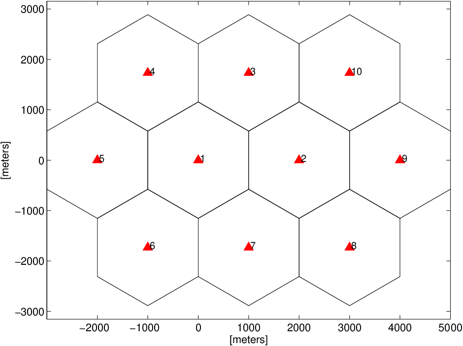
Refer to caption — Fig. 1: Network configuration

In the following numerical experiments, we consider HetNets with at most $10$ cells. The distance between centers of adjacent cells is set as $2000$ meters; see Fig. 1 for an illustration of the network configuration. In each cell, we place one BS at the center of the cell (representing the macro BS), and randomly and uniformly place $I$ users and $Q-1$ remaining BSs. The channel model we use is Rayleigh channel with zero mean and variance $(200/d_{i_{k}}^{q_{l}})^{3}L_{i_{k}}^{q_{l}},$ where $d_{i_{k}}^{q_{l}}$ is the distance between BS $q_{l}$ and user $i_{k}$ , and $10\log 10(L_{i_{k}}^{q_{l}})\sim N(0,64)$ . We also assume that $\sigma_{i_{k}}^{2}=\sigma^{2},~~\forall i_{k}\in\mathcal{I}$ . All the simulation results are averaged over $100$ channel realizations. The results shown for problem (8), (34) and (47) are those obtained after performing the de-biasing step. The proposed algorithm is compared to the following two scenarios: 1) all the BSs are turned on; 2) in each cell, the central BS and a randomly selected fixed number of the remaining BSs are turned on. Note that for both of these cases, full JP is used within each cell. Clearly, the first scenario can serve as the performance upper bound, and the latter can serve as a reasonable heuristic algorithm to select active BSs since BSs and users are uniformly distributed in each cell.

In the first set of simulations, the total power minimization design criterion is considered. We set $I=10$ , $Q=20$ , $M=5$ , and $\tau_{i_{k}}=15$ dB, $~\forall i_{k}\in\mathcal{I}$ . Furthermore, we assume that the power budget for BSs in the center of each cell is $10$ dB while the budget for the rest of the BSs is set to be $5$ dB. We apply the ADMM approach to solve the proposed formulation (8) with reweighting procedure. Since the objective QoS $\tau_{i_{k}},~~\forall i_{k}\in\mathcal{I}$ may not always be feasible, we declare that this realization is infeasible if a particular problem realization cannot converge within $2000$ ADMM iterations. We select the stepsize as $\rho=5$ , and use the following stopping criterion

\displaystyle\max\left(\left\|\frac{\|vec({\bf K})\|_{\infty}}{\max(1,\|{\bf K}\|_{F})}\right\|,\left\|\frac{{\bf v}-{\bm{w}}}{\max(1,\|{\bf v}\|,\|{\bm{w}}\|)}\right\|_{\infty},\max_{i_{k}\in\mathcal{I}}(|\kappa_{i_{k}}^{2}-\sigma^{2}|),\frac{f^{\min}({\bm{w}}^{(t)})-f^{\min}({\bm{w}}^{(t-1)})}{f^{\min}({\bm{w}}^{(t-1)})}\right)<10^{-4}.

In Fig. 2, we plot the number of active BSs after each reweighting procedure on $\beta_{q_{k}},~~\forall q_{k}\in\mathcal{Q}$ for $1/\sigma^{n}=5$ dB and $10$ dB, respectively. From this figure, it can be observed that the number of active BSs decreases fast for the first $2$ reweighting iterations, and converges within $6$ reweighting iterations. In Fig. 3, the obtained minimum total power is plotted against the number of cells. We can observe that the minimum required power for BSs selected by the proposed formulation (8) is more than that achieved by activating all the BSs in each cell. This is reasonable since the latter serves as a lower bound of achievable power consumption. On the other hand, when $1/\sigma^{2}=10$ dB, we compare the minimum power consumption achieved by the following two networks: i) a network with $70\%$ of randomly activated BSs (the center BSs in each cell are always active) and ii) the network optimized by the proposed algorithm ( $35.8\%\sim 43.45\%$ of BSs are activated for each number of cells). It can be observed that the proposed formulation is able to use much smaller number of BSs with similar total transmit power to support the same set of QoS constraints. This demonstrates the efficacy of the proposed method. Additionally, Fig. 4 plots the required number of ADMM iterations for the power minimization only design (4) (with all BSs being turned on). We observe that the proposed ADMM approach converges fairly fast. Note that the convergence speed depends on the channel quality, $\sigma^{2}$ : when the channel condition is good enough, i.e., $1/\sigma^{2}=10$ dB, it converges within $250$ ADMM iterations.

Number of Cells	4	6	8	10
WMMSE (all BSs)	40	60	80	100
Random BSs Selection ( $50\%$ BSs)	20	30	40	50
S-WMMSE ( $\mu=1.5$ , $\lambda=0$ ), $P^{tot}=10$ dB	18.27	26.33	35.24	43.53
S-WMMSE ( $\mu=1$ , $\lambda=0.25$ ), $P^{tot}=10$ dB	20.18	28.67	38.51	47.04
S-WMMSE ( $\mu=2.5$ , $\lambda=0$ ), $P^{tot}=30$ dB	21.11	28.38	36.42	45.80
S-WMMSE ( $\mu=2.5$ , $\lambda=0.05$ ), $P^{tot}=30$ dB	20.21	28.73	37.80	46.95

TABLE I: The number of active BSs v.s. different number of cells.

In the second simulation set, the sum rate maximization design criterion is investigated. Let $I=10$ , $Q=10$ , $M=4$ , $N=2$ and $P^{tot}$ denote the total power budget in each cell. The power budget for BSs located in the center of the cells is $P^{tot}/2$ , and the rest of the BSs have equal power budgets. For simplicity, we set $\mu_{q_{k}}=\mu,~~\forall q_{k}\in\mathcal{Q}$ , $\lambda_{k}=\lambda,~~\forall k\in\mathcal{K}$ , and $\sigma_{i_{k}}^{2}=1,~~\forall i_{k}\in\mathcal{I}$ . The reweighting procedure is performed until no BS reduction is possible or less than $50\%$ of BSs is active. This is for fair comparison with random selection scheme turning on $50\%$ of BSs. In Fig. 5, the system sum rate performance for the proposed S-WMMSE algorithm is compared with $P^{tot}=10$ dB and $30$ dB. We can observe that S-WMMSE can achieve about 80% of the sum rate compared to the upper bound while activating around 50% BSs (see Tab. I for details about the number of active BSs). Furthermore, while the number of active BSs for S-WMMSE is about the same as the random selection scheme, the S-WMMSE can still achieve more than 34% and 23% improvement in sum rate performance for $P^{tot}=10$ dB and $30$ dB, respectively. It is worth noting that when BS clustering is considered, there is no sizable decrease in the sum rate performances. However, the total power consumption is significantly reduced; see Fig. 6. This is because when optimizing the BS clustering, the coverage of each BS is reduced, so does the interference level. As a result, less total transmit power is able to support similar sum rate performance.

In summary, our simulation results suggest that for the power minimization design criterion, the proposed ADMM approach can effectively reduce the BS usage while minimizing the required minimum power consumption. On the other hand, when considering the sum rate maximization design criterion, the proposed S-WMMSE algorithm can effectively reduce the BS usage and the size of BS cluster simultaneously.

VI Concluding Remarks

In this paper, we have considered the downlink beamforming problems that jointly select the active BSs while C1) minimizing the total power consumption; or C2) maximizing the sum rate performance. Since the considered problems are shown to be strongly NP-hard in general, we have utilized the sparse-promoting techniques and proposed formulations that effectively select the active BSs. Moreover, for these two design criteria, we have developed efficient distributed algorithms that are based on respectively the ADMM algorithm and WMMSE algorithm. Interestingly, when specialized to the standard problem of minimum power MISO downlink beamforming without BS selection(see [16, 17]), our proposed ADMM approach is more efficient than the conventional approach that exploits the uplink-downlink duality [20, 16, 17] with computation complexity analysis. For future work, it would be interesting to apply the ADMM approach to efficiently solve general large-scale SOCPs, and to consider downlink beamforming problems and algorithms for situations where only long-term channel statistics are available.

-A Proof of Theorem 1

To prove Theorem 1, it is sufficient to show that problem (6) is strongly NP-hard. Consider a simple single-cell network with $Q$ single antenna BSs serving $Q$ users. That is, $K=1$ , $M=1$ , $|\mathcal{Q}_{k}|=|\mathcal{I}_{k}|=Q$ . Then problem (6) can be simplified to

$\displaystyle\min_{\{p_{i}^{q}\}}~$	$\displaystyle\sum_{i=1}^{Q}\left\\|\sum_{q=1}^{Q}p_{i}^{q}\right\\|_{0}$
$\displaystyle\rm{s.t.}~$	$\displaystyle\frac{\sum_{q=1}^{Q}p_{i}^{q}g_{i}^{q}}{\sigma_{i}^{2}+\sum_{j\neq i}\sum_{q=1}^{Q}p_{j}^{q}g_{i}^{q}}\geq\tau_{i},$	(48)
	$\displaystyle\sum_{i=1}^{Q}p_{i}^{q}\leq P_{q},~p_{i}^{q}\geq 0,~~\forall~i,q=1,\ldots,Q,$

where we have omitted the cell index $k$ , and have defined $p_{i}^{q}\triangleq\|{\bf v}_{i}^{q}\|_{2}^{2}\mbox{~and~}g_{i}^{q}\triangleq\|{\bf h}_{i}^{q}\|_{2}^{2},~~\forall i,q=1,\ldots,Q$ . We prove that problem (48) is strongly NP-hard by establishing a polynomial time transformation from the so-called vertex cover problem. The vertex cover problem can be described as follows: given a graph $\mathcal{G}=(\mathcal{V},\mathcal{E})$ and a positive integer $N\leq|\mathcal{V}|$ , we are asked whether there exists a vertex cover of size $N$ or less, i.e., a subset $\mathcal{V}^{\prime}\subset\mathcal{V}$ such that $|\mathcal{V}^{\prime}|\leq N$ , and for each edge $\{u,v\}\in\mathcal{E}$ at least one of $u$ and $v$ belongs to $\mathcal{V}$ .

Given a graph $\mathcal{G}=(\mathcal{V},\mathcal{E})$ with $|\mathcal{V}|=Q$ , we let

		$\displaystyle g_{i}^{q}=g_{q}^{i}=\left\{\begin{array}[]{ll}1,&\mbox{if}~i=q~\mbox{or}~(i,q)\in\mathcal{E}\\ 0,&\mbox{if}~(i,q)\not\in\mathcal{E}\end{array}\right.$
		$\displaystyle\tau_{i}=\frac{1}{Q^{2}},~\sigma_{i}^{2}=Q,~P_{q}=Q,~~\forall q=1,\ldots,Q.$

We claim that the optimal value of problem (48) is less than or equal to $N$ if and only if there exists a vertex cover set $\mathcal{V}^{\prime}$ for the graph satisfying $|\mathcal{V}^{\prime}|\leq N$ .

“If” direction: Let $\mathcal{V}^{\prime}$ with $|\mathcal{V}^{\prime}|\leq N$ be the vertex cover set for the graph $\mathcal{G}$ . Without loss of generality, suppose $\mathcal{V}^{\prime}=\{1,2,\ldots,N\}$ . Then we can construct a feasible solution for problem (48) based on the cover set $\mathcal{V}^{\prime}$ such that the optimal value of problem (48) at this point is equal to $N$ . In particular, we have

		$\displaystyle p_{i}^{q}=1,~i=1,\ldots,Q,~q=1,2,\ldots,N$
		$\displaystyle p_{i}^{q}=0,~i=1,\ldots,Q,~q=N+1,N+2,\ldots,Q$

Next, we check the feasibility of the above constructed solution.

•

For user $i=1,2,\ldots,N$ , the SINR constraint in (48) is satisfied, since $p_{q}^{q}=g_{q}^{q}=1$ for all $q=1,\ldots,N$ .
•

For user $i=N+1,N+2,\ldots,Q$ , according to the definition of the cover set, there must exist $q\in\mathcal{V}^{\prime}$ such that $(i,q)\in\mathcal{E}$ and thus $p_{i}^{q}=g_{i}^{q}=1$ . Hence, the SINR constraint of user $i=N+1,N+2,\ldots,Q$ are also satisfied.

“Only if” direction: Suppose that the optimal value of problem (48) is less than or equal to $N$ and its optimal solution is $p_{i}^{q\star},~~\forall i,q=1,\ldots,Q$ . We construct the following sets

\displaystyle S_{q}\triangleq\{i\mid p_{i}^{q\star}g_{i}^{q}>0\}=\{i\mid p_{i}^{q\star}>0\},~q=1,\ldots,Q.

By the fact that the optimal value of problem (48) is less than or equal to $N$ , we know that at most $N$ of the defined sets $S_{q}$ are nonempty sets. Without loss of generality, suppose these $N$ nonempty sets are $S_{1},\ldots,S_{N}$ . Furthermore, the fact that all SINR constraints are satisfied implies

\displaystyle\mathcal{V}=\bigcup_{q=1}^{Q}S_{q}=\bigcup_{q=1}^{N}S_{q}.

The above shows that $\{1,2,\ldots,N\}$ constitutes a cover set of $\mathcal{V}$ , which completes the proof. $\Box$

References

[1] W.-C. Liao, M. Hong, and Z.-Q. Luo, “Base station activation and linear transceiver design for utility maximization in heterogeneous networks,” in Proc. of IEEE International Conference on Acoustics, Speech and Signal Processing (ICASSP), Vancouver, May 26-31 2013, pp. 4419–4423.
[2] A. Damnjanovic, J. Montojo, Y. Wei, T. Ji, T. Luo, M. Vajapeyam, T. Yoo, O. Song, and D. Malladi, “A survey on 3GPP heterogeneous networks,” IEEE Trans. Wireless Communications, vol. 18, no. 3, pp. 10–21, Jun. 2011.
[3] M. Hong and Z.-Q. Luo, “Signal processing and optimal resource allocation for the interference channel,” EURASIP E-Reference Signal Processing, 2012, accepted, available at http://arxiv.org.
[4] B. Clerckx, A. Lozano, S. Sesia, C. van Rensburg, and C. B. Papadias, “3GPP LTE and LTE Advanced,” EURASIP Journal on Wireless Communications and Networking, 2009.
[5] D. Gesbert, S. Hanly, H. Huang, S. Shamai, O. Simeone, and W. Yu, “Multi-cell MIMO cooperative networks: A new look at interference,” IEEE J. Sel. Areas in Communications, vol. 28, no. 9, pp. 1380–1408, Dec. 2010.
[6] J. Zhang, R. Chen, J. Andrews, A. Ghosh, and R. Heath, “Networked mimo with clustered linear precoding,” IEEE Trans. Wireless Communications, vol. 4, no. 8, pp. 1910–921, Jun. 2009.
[7] A. Papadogiannis, D. Gesbert, and E. Hardouin, “A dynamic clustering approach in wireless networks with multi-cell cooperative processing,” in Proc. of IEEE International Conference on Communications, May 2008, pp. 4033–4037.
[8] A. Papadogiannis and G. Alexandropoulos, “The value of dynamic clustering of base stations for future wireless networks,” in IEEE International Conference on Fuzzy Systems (FUZZ), Jul. 2010, pp. 1–6.
[9] Y. Zeng, E. Gunawan, Y.-L. Guan, and J. Liu, “Joint base station selection and linear precoding for cellular networks with multi-cell processing,” in TENCON, Nov. 2010, pp. 1976–1981.
[10] S.-J. Kim, S. Jain, and G. B. Giannakis, “Backhaul-constrained multi-cell cooperation using compressive sensing and spectral clustering,” in Proc. of IEEE 13th International Workshop on Signal Processing Advances for Wireless Communications, Cesme, Jun. 17-20 2012, pp. 65–69.
[11] M. Hong, R. Sun, and Z.-Q. Luo, “Joint base station clustering and beamformer design for partial coordinated transmission in heterogenous networks,” IEEE Journal on Selected Areas in Communications, vol. 31, no. 2, pp. 226–240, Feb. 2013.
[12] Y. Cheng, M. Pesavento, and A. Philipp, “Joint network optimization and downlink beamforming for comp transmissions using mixed integer conic programming,” IEEE Trans. Signal Process., vol. 61, no. 16, pp. 3972–3987, Aug. 2013.
[13] O. Arnold, F. Richter, G. Fettweis, and O. Blume, “Power consumption modeling of different base station types in heterogeneous cellular networks,” in Proc. of Future Network and Mobile Summit, Jun. 2010, pp. 1–8.
[14] O. Mehanna, N. D. Sidiropoulos, and G. B. Giannakis, “Multicast beamforming with antenna selection,” in Proc. of IEEE 13th International Workshop on Signal Processing Advances for Wireless Communications, Cesme, Jun. 17-20 2012, pp. 70–74.
[15] Y.-F. Liu, Y.-H. Dai, and Z.-Q. Luo, “Joint power and admission control via linear programming deflation,” IEEE Trans. Signal Process., vol. 61, no. 6, pp. 1327–1338, Mar. 2013.
[16] A. Wiesel, Y. C. Eldar, and S. Shamai, “Linear precoding vis conic optimization for fixed MIMO receivers,” IEEE Trans. Signal Process., vol. 54, no. 1, pp. 161–176, Jan. 2006.
[17] H. Dahrouj and W. Yu, “Coordinated beamforming for the multicell multi-antenna wireless system,” IEEE Trans. Wireless Communications, vol. 9, no. 5, pp. 1748–1759, May 2010.
[18] D. P. Bertsekas and J. N. Tsitsiklis, Parallel and Distributed Computation: Numerical Methods. Athena Scientific, 1997.
[19] S. Boyd, N. Parikh, E. Chu, B. Peleato, and J. Eckstein, “Distributed optimization and statistical learning via the alternating direction method of multipliers,” Foundations and Trends in Machine Learning, vol. 3, no. 1, pp. 1–122, 2011.
[20] F. Rashid-Farrokhi, K. J. R. Liu, and L. Tassiulas, “Transmit beamforming and power control for cellular wireless systems,” IEEE J. Sel. Areas in Communications, vol. 16, no. 8, pp. 1437–1450, Oct. 1998.
[21] S. Joshi, M. Codreanu, and M. Latva-aho, “Distributed resource allocation for MISO downlink systems via the alternating direction method of multipliers,” in Proc. IEEE Asilomar Conf. on Signals, Systems, and Computers, 2012, pp. 488–493.
[22] C. Shen, T.-H. Chang, K.-Y. Wang, Z. Qiu, and C.-Y. Chi, “Distributed robust multicell coordinated beamforming with imperfect csi: An admm approach,” IEEE Trans. Signal Process., vol. 60, no. 6, pp. 2988–3003, Jun. 2012.
[23] Q. Shi, M. Razaviyayn, Z.-Q. Luo, and C. He, “An iteratively weighted mmse approach to distributed sum-utility maximization for a MIMO interfering broadcast channel,” IEEE Trans. Signal Process., vol. 59, no. 9, pp. 4331–4340, Sep. 2011.
[24] Z.-Q. Luo and S. Zhang, “Dynamic spectrum management: Complexity and duality,” IEEE J. Sel. Topics Signal Process., vol. 2, no. 1, pp. 57–73, Feb. 2008.
[25] M. Yuan and Y. Lin, “Model selection and estimation in regression with grouped variables,” Journal of the Royal Statistical Society: Series B, vol. 68, no. 1, pp. 49–67, Feb. 2006.
[26] M. Grant and S. Boyd, “CVX: Matlab software for disciplined convex programming,” http://stanford.edu/ $\sim$ boyd/cvx, June 2009.
[27] S. J. Wright, R. D. Nowak, and M. A. T. Figueiredo, “Sparse reconstruction by separable approximation,” IEEE Trans. Signal Process., vol. 57, no. 7, pp. 2479–2493, Jul. 2009.
[28] E. Candes, M.Wakin, and S. Boyd, “Enhancing sparsity by reweighted $l_{1}$ minimization,” J. Fourier Analysis and Applications, vol. 14, no. 5, pp. 877–905, Dec. 2008.
[29] P. Tseng, “Convergence of a block coordinate descent method for nondifferentiable minimization,” Journal of Optimization Theory and Applications, vol. 109, no. 3, pp. 475–494, Jun. 2001.