(Failure of the) Wisdom of the crowds in an endogenous opinion dynamics model with multiply biased agents
Abstract
We study an endogenous opinion (or, belief) dynamics model where we endogenize the social network that models the link (‘trust’) weights between agents. Our network adjustment mechanism is simple: an agent increases her weight for another agent if that agent has been close to truth (whence, our adjustment criterion is ‘past performance’). Moreover, we consider multiply biased agents that do not learn in a fully rational manner but are subject to persuasion bias — they learn in a DeGroot manner, via a simple ‘rule of thumb’ — and that have biased initial beliefs. In addition, we also study this setup under conformity, opposition, and homophily — which are recently suggested variants of DeGroot learning in social networks — thereby taking into account further biases agents are susceptible to. Our main focus is on crowd wisdom, that is, on the question whether the so biased agents can adequately aggregate dispersed information and, consequently, learn the true states of the topics they communicate about. In particular, we present several conditions under which wisdom fails.
1 Introduction
Crowds can be amazingly wise, even wiser than the most accurate individuals among them. An early formalization of this insight has been Concordet’s Jury theorem from 1785 [22], which states that a simple majority vote of the opinions of independent and fallible lay-people may provide near-perfect accuracy if the number of voters is sufficiently large.11 1 Which also requires that each individual in the group of voters is more likely correct than not. Over a hundred years later, in 1906, Francis Galton [38] found strong empirical support of Concordet’s theoretical finding at an agricultural fair in Plymouth. At a weight-judging contest, participants were asked to privately estimate the weight of a chosen live ox after it had been slaughtered and dressed (meaning that the head and other parts were removed). The winner was the one whose estimate was closest to the true weight of the ox. When analyzing the results in a Nature article the following year, Galton found that the simple average of the entire crowd was even more accurate than the winner and that the median of the valid guesses, pounds, was extremely close to the true weight, pounds (cf. Bahrami, Olsen, Bang, Roepstorff, Rees, and Frith (2012) [7], Acemoglu and Ozdaglar (2011) [3]). This finding was obtained even though most participants were no ‘experts’ in this contest, with little specialized knowledge in butchery; yet, their estimates could obviously contribute to the crowds’ overall success. Galton took this result as evidence that democratic political systems may work.
Yet, contradicting this optimistic viewpoint concerning the wisdom of crowds, it has also been observed that groups of individuals may be quite fallible, and possibly even more fallible than most or all of their members. One result of this kind is already hidden in Concordet’s Jury theorem: namely, if each lay-person is just slightly ‘too uniformed’ (or slightly ‘too much mistaken’), then the majority vote may be much less accurate than each individual’s estimate. Drawing upon empirical observations, a comprehensive illustration of ‘crowd madness’ has been brought forward in Scottish journalist Charles Mackay’s (1841) [63] work The extraordinary and popular delusions and the madness of crowds, where the author chronicles ‘humankind’s collective follies’, including financial bubbles, in the economics context, and other popular ‘delusions’ such as witch-hunts and fortune-telling (cf. Bahrami, Olsen, Bang, Roepstorff, Rees, and Frith (2012) [7]), thus challenging the claim that “two heads are better than one”.
Today --- while, according to scholars’ opinions, the question of wisdom of crowds continues to be one of the most important issues facing social sciences in the twenty-first century ---22 2 See the recent survey at http://bit.ly/hR3hcS. more is known on group wisdom and collective failure. On the one hand, the mean of the opinions of several individuals may become increasingly accurate, for large groups, merely as a consequence of the law of large numbers. This holds under restrictive assumptions — in particular, that the beliefs of individuals are independent and probabilistically centered around truth such that, on an aggregate level, individual errors cancel out. On the other hand, much empirical literature, foremostly in psychology, has documented that, frequently, “groups outperform individuals […], although groups typically fall short of the performance of their highest-ability members” (Kerr, MacCoun, and Kramer (1996) [51], p.691).33 3 Groups can also blatantly fail, as, e.g., in groupthink (Janis (1972) [48]), hidden profiles (Wittenbaum and Stasser (1996) [72]), etc. See the overview in Kerr and Tindale (2004) [52]. In fact, a very recent experiment by Lorenz, Rauhut, Schweitzer, and Helbig (2011) [62] finds that ‘social influence’, in a broad meaning, in a group causes individuals’ beliefs to become more similar over time, without improvements in accuracy, however. Hence, much depends on how groups aggregate or process individual opinions and also on these initial predispositions of agents. Kerr, MacCoun, and Kramer’s (1996) [51] insight is that whether groups perform better than individuals may depend, among other things, on the following aspects: (1) the way that groups aggregate the opinions of individuals (that is, the group decision, or belief integrating, process), (2) the bias of individuals, and (3) the type of bias. Concerning issue (1), the way agents in groups process their peers’ beliefs, we assume a specific structural form below, which has empirically proved plausible for learning in the domain we consider (social networks).
Issue (2), individuals’ bias, will be another central notion in our work. The classical work of Tversky and Kahnemann (1974) [70] documents several biases human judgment is susceptible to. In particular, anchoring biases describe the psychological condition of humans to pay undue attention to initial values — e.g., typically, individuals estimate the product to be higher than the product of factors in reverse order, which is attributed to subjects’ performing an initial approximate computation based on the first few terms, which entails a biasing anchor (the same effects may happen if the anchor is exogenously specified, e.g., by providing the subjects with random numbers as anchors and then querying them for their own judgement). Biases of availabilty refer to the phenomenon of assessing (and, consequently, possibly, misjudging) the probability of an event by the ‘ease with which instances or occurrences can be brought to mind’, and, finally, biases of representativeness lead subjects to assess the probability that an object is of a particular class (e.g., that a person has a certain profession) by the degree to which the object is representative of the class, which may lead to judgement errors because such reasoning ignores, e.g., base-rate frequencies. In another typological classification of bias, Kerr, MacCoun and Kramer (1996) [51] distinguish between judgmental sins of imprecision (systematically deviating from prescribed and precise use of information, such as ignoring Bayes’ theorem when forming beliefs or being affected by framing; see Kahnemann and Tversky, 1984 [50]), judgmental sins of commission (using irrelevant information to arrive at a decision, such as the attractiveness of an accused) and judgmental sins of omission (ignoring relevant information, such as base-rate information).
We now describe the setup investigated in the current work, relating to the issues discussed above subsequently. We consider a (social) network of individuals, or agents, that form opinions, or beliefs, about an underlying state or a discussion topic.44 4 Opinions or beliefs are important, from an economics perspective, because they crucially shape economic behavior: consumers’ opinions about a product determine the demand for that product and majority opinions set the political course, etc. See Buechel, Hellmann, and Klößner (2013) [15]. We assume that agents start with some initial beliefs, at time zero, and then, as time progresses, learn from each other through communication. Communication between any two individuals takes place if there is a link between them in the network. In the current work, we assume a specific form of learning paradigm, DeGroot learning, that posits that agents update their beliefs by taking weighted arithmetic averages of their peers’ past beliefs, whereby the weights are given by the (social) ties between the agents in the network. Much has been said on the adequacy (or inadequacy) of DeGroot learning — a ‘boundedly rational’ learning paradigm that posits that agents are susceptible to persuasion bias, not properly adjusting for the repetition of information they hear — which, as experiments claim (e.g., [19, 21]), appears as a more plausible standard of human social learning than, e.g., fully rational Bayesian learning and we refer the reader to, e.g., DeMarzo, Vayanos, and Zwiebel (2003) [25], Golub and Jackson (2010) [39] or Acemoglu and Ozdaglar (2011) [3] for extensive discussions. While the DeGroot model of opinion formation is quite old, dating back to Morris H. DeGroot (1974)’s [24] seminal work, the framework has only more recently received increasing attention from the economics community.
In this context, one matter that has been put forth as a central guiding question in DeGroot learning models, and which connects to our initial discussion, is whether the ‘naïve’ DeGroot learners, who commit the ‘sin of imprecision’ of not (properly) applying Bayes’ theorem, can, in fact, become ‘wise’ [39]. Here, a society (set of agents) is called wise, roughly, if it reaches a consensus — in the limit, as time (discussion periods) goes to infinity — that corresponds to truth. In Golub and Jackson (2010) [39], the question relating to wisdom has been answered in the affirmative — (even) naïve (DeGroot) learners do become wise under rather mild conditions; namely, all that is required is that no naïve learner is excessively influential, whereby an agent is excessively influential if his social influence (how limiting beliefs depend on this agent’s initial beliefs) does not converge to zero as society grows. In undirected networks (social ties are mutual) with uniform weights, an obstacle to wisdom would then, e.g., be that each agent newly entering society assigns, e.g., a constant fraction of his links to a particular agent, who would then be excessively influential. Hence, as long as links are somewhat ‘democratically’ balanced, naïve DeGroot learners would apparently become wise. While we hold the analysis of Golub and Jackson (2010) [39] to be an important ‘benchmark’ for DeGroot learning, we think that it is overly optimistic in at least one of its critical two assumptions, namely, the (1) unbiasedness of agents’ initial beliefs.55 5 The other critical assumption is biasedness of the belief formation process (DeGroot learning — agents are prone to persuasion bias). Finally, of crucial relevance is also independence of agents’ initial beliefs, which we do not challenge here, however.
In the current work, we drop, in particular, the largely implausible, as we find, assumption (1). Our central notion will be as illustrated in Figure 1, which we adapt from Einhorn, Hogarth, and Klempner (1977) [31].
In words, we assume that some agents’ initial beliefs are biased, with an expected value that is different from truth , and that other agents’ initial beliefs are unbiased, with an expected value that equals truth — we remark here that we abstract away from the precise type of bias some agents’ initial beliefs are subject to, that is, we are agnostic about whether, e.g., agents commit sins of imprecision, commission, or omission in forming their initial beliefs, simply assuming that at least some agents’ initial beliefs are biased. We might, if we wish, label the first kind of agents ‘non-experts’ and the second ‘experts’, although this might be slightly misleading, as even experts can be biased, of course; nonetheless, for convenience, we keep this terminology in the following. A situation as sketched may be quite challenging to assess, for individuals. Ignoring non-experts may be suboptimal, in some circumstances, because their verdicts may still not be totally irrelevant in that their opinions may have (relatively) large probability of being close to truth. Consider, in particular, the bottom part of Figure 1 where the ‘expert’ is unbiased but has high variance. In this case, for each ‘closeness interval’ around truth, the non-expert’s initial belief has higher probability of falling within this interval than the expert’s beliefs. Thus, if there is exactly one expert and one non-expert, it would be optimal, for an outside observer, to disregard the expert’s opinion and, in the absence of further information, adopt the non-expert’s opinion. However, if there are many experts with identical and independent distributions and also many non-experts with identical and independent distributions, then an optimal aggregation of information would ignore the non-experts’ and average the experts’ opinions.
We study this setup in an endogenous DeGroot learning model, where we endogenize the (social) network. In particular, we assume that the ‘trust’ links between agents in the network are based on ‘past performance’, which has been outlined as a relevant reputation building criterion in the psychology literature (cf. Yaniv and Kleinberger (2000) [74], Yaniv (2004) [73]). We think that the endogenous model is the ‘right’ setup for our investigation of wisdom in DeGroot learning under biased initial beliefs because if the network structure is assumed exogenous, then one relatively uninteresting solution to the wisdom problem would, e.g., be to ignore the biased agents — in contrast, in the endogenous model, the question arises what weighting scheme individuals actually learn for the biased (and unbiased) agents, under given assumptions concerning the agents’ behavior. Since we learn the network structure endogenously, by looking at agents’ past performance (how often have they been close to truth previously?), we necessarily study learning in a repeated setting, where agents are involved in repeated communications over multitudes of topics, whereby past beliefs and their external validation may inform today’s beliefs and the network structure. Our network learning rule is quite simple: we increment the weight that one agent places upon another by some if the latter agent has been in a predefined ‘-radius’ around truth for the current topic. We show that this is a ‘utility maximizing’ rule66 6 Or at least a good approximation to a solution of a maximization problem. provided that agents expect, subjectively, that all other agents’ beliefs are unbiased, which we call the bona fides (or, ‘good faith’) assumption. Intruigingly, the bona fides assumption concerning the unbiasedness of other agents’ initial beliefs may be consistent with the ‘egocentric bias’ hypothesis which suggests that “interacting human agents operate under the assumption that their collaborators’ decisions and opinions share the same level of reliability” as their own; the upholding of this bias, even despite potential collective failure, might then be due to the social obligation to treat others as equal to oneself, despite their conspicuous inadequacy, or due to the urge to contribute to the group (Bahrami, Olsen, Bang, Roepstorff, Rees, and Frith (2012) [7]).
To summarize our model, in our setup, agents hold beliefs and learn, via communication, about a multitude of topics , each with an associated ‘truth’ . Within each topic , ‘discussion rounds’ are indexed by discrete time steps and in each time step , agents update their beliefs on by integrating their peers’ beliefs, starting with some exogenously specified initial beliefs on . After a topic has been communicated about (for an infinite amount of time), truth is revealed, whereupon agents adjust the ‘trust’ weights they assign to other agents (they ‘learn’, or ‘grow’, the network topology) based on agents’ past performance: if an agent has been close to truth for topic , agents increase their trust for this agent by increasing the respective weight by . Our agents are multiply biased (or ‘naïve’):
- (i)
At least some agents’ initial beliefs are systematically biased in that the expected values of their initial beliefs are different from truth , for all . For initial beliefs, we abstract away from the particular kind of bias agents are subject to, simply assuming that some kind of bias plays a role.
- (ii)
Agents are subject to persuasion bias in updating their beliefs on in that they apply the DeGroot learning paradigm rather than a fully rational Bayesian belief updating framework.
- (iii)
In adjusting weights for other agents, agents are egocentrically biased: they assume that their own judgments are relevant (more precisely, their initial beliefs are unbiased) and they assume that their peers’ beliefs share the same level of reliability as their own (more precisely, that their peers’ initial beliefs are also unbiased). This bias justifies the weight adjustment rule — adding — that we have sketched (see Section 3).
Besides this basic setup, we consider refinements of standard DeGroot learning recently suggested — DeGroot learning under opposition, conformity, and homophily — in each case incorporating our endogenized network structure and, in addition, the three kinds of biases discussed above. We show that, in these more refined versions of DeGroot learning, which are supposed to endow the DeGroot learning paradigm with a more ‘realistic’ structure, wisdom is even more difficult to arrive at, as we discuss below.
Our main contributions over existing work are as follows.
- •
We more thoroughly investigate the concept of bias in social (network) learning — or more specificially, DeGroot learning — than previous literature. In particular, as mentioned, we allow agents’ initial beliefs to be biased and consider further biases, as discussed.
- •
We endogenize the network structure in DeGroot learning and we do so by referring to the notion of ‘past performance’. Of course, in the vast literature on networks, (‘endogenous’) network formation processes are not novel; often, however, the network is adapted, in the literature more or less relevant to our setup, by adding or deleting (costly) links as in Jackson and Watts (2002) [47], Goyal (2004) [41], etc., rather than by increasing link weight based on agents’ past performance. In DeGroot learning, self-evolving networks are discussed, e.g., in the work on DeGroot learning and homophily (e.g., Pan (2010) [67] and the Hegselmann and Krause models), but weight adjustments based on truth, as we model, must be considered distinct from these mechanisms.
- •
As mentioned, we consider multitudes of topics, rather than a single topic, in DeGroot learning, and we crucially allow truth to be revealed at some stage. This differs from all the previous work, where agents have been in the unfortunate situation of eternally communicating about a given topic, without ever knowing its true state.
- •
- •
We derive a microeconomic foundation for weight adjustments as we implement by defining an individual agent’s optimization problem --- in particular, we assume that agents have negative utility from not knowing truth --- and by computing a closed-form solution to this problem.77 7 In spirit, our approach is similar to that of DeMarzo, Vayanos, and Zwiebel (2003) [25]. We then show how our heuristic weight adjustment rule — adding — corresponds to the solution of the optimization problem.
Our main findings are as follows.
- •
For the standard model, we first show that agents reach a consensus for almost all topics , under weak conditions, in our endogenized DeGroot learning paradigm (Proposition 6.1 and Remark 6.2). This confirms the commonly held belief (cf. Acemoglu and Ozdaglar (2011) [3]) that the standard DeGroot model leads agents to consensus (so easily) but also shows that, in our endogenized model, conditons that prevent consensus are, in fact, not satisfied.
- •
Next, we illustrate that if all agents’ initial beliefs are unbiased, then agents in fact reach a consensus that is even correct, for ‘large’ topics and as agent group size becomes large. This holds both when agents adjust weights based on limiting beliefs and on initial beliefs (Propositions 6.3 and 6.4, respectively); we define the notions of relevant weight adjustment time points below. When there are biased agents, then agents’ limiting beliefs are generally a convex combination of the unbiased agents’ initial beliefs and the biased agents’ initial beliefs. We demonstrate the truthfulness of this claim under various parametrizations (Propositions 6.5, 6.7, 6.8). We also give sufficient conditions on when agents may converge to truth, for large topics, even under the presence of biased agents (Propositions 6.5 and 6.6), but these conditions are ‘low probability events’ (or require a sufficiently high valuation of truth) and they hold only under the particular parametrization that agents stop learning the network topology in case ‘everything is fine’, as we define below.
That limiting consensus beliefs are convex combinations of biased and unbiased beliefs may imply that limiting beliefs are ‘arbitrarily’ far off from truth, provided that the number of biased agents is sufficiently large (Corollary 6.3), thus demonstrating that agents do not optimally aggregate information in our endogenized DeGroot learning model, at least under certain conditions.
- •
Next, for opinion dynamics ‘under opposition’, a recently suggested DeGroot learning variant where agents are motivated by ‘ingroup’/‘outgroup’ relationships [30], we show that even if all agents’ initial beliefs are unbiased and, more particularly, agents receive arbitrarily accurate initial signals about topics, some agents may be arbitarily far off from truth. In other words, we show that if agents have additional incentives besides truth, namely, to disassociate from unliked others --- such agents must be thought of as additionally biased; namely, they must be thought of as, e.g., committing the sin of omission to ignore the unliked others’ relevant information and the sin of commission to incorporate irrelevant information, namely, the ‘opposite’ of unliked others’ beliefs ---88 8 They may generally be thought of as biased toward ingroup members, cf. Brewer (1979) [12]. then wisdom is even more difficult to attain. This, in particular, concerns several important fields of everyday life, such as the political arena.
- •
Then, for DeGroot learning ‘under conformity’ — that is, when agents want to conform to a reference opinion (again, which may be thought of as a sin of commission) — another recent variant of DeGroot learning [14], we show that even if the unbiased agents have never been truthful in the past, they may become arbitrarily influential, something that is not possible in the standard model, and which, again, shows that additional biases may worsen the case for wisdom.
- •
Finally, in case homophily also plays a role — that is, when agents have the tendency to adjust the social network topology based on agents with similar beliefs — then, again, wisdom is more difficult to arrive at. We show this (only) by simulation since this process is (much) more difficult to analyze analytically as it deals with learning matrices that are changing over time (and not only across topics). In our context, homophily can also be seen as a search bias in which subjects overrate beliefs that are close to their own (cf. Kunda (1990) [55]).
The structure of this work is as follows. In Section 2, we present related work, beyond what we have already referred to. In Section 3, we give a formal outline of our model, and, in Section 4, a ‘justification’ of our network learning rule. In Section 5, we introduce relevant notation. Then, in Sections 6, 7, 8, and 9, we derive our results, as outlined above, on the standard model, and the DeGroot variants under opposition, conformity, and homophily, respectively. In Section 10, we conclude. We list several proofs in the appendices; there, we also report on a ‘small-scale’ experiment on the (un)biasedness (and the distribution) of individuals’ (initial) beliefs concerning several ‘common knowledge questions’.
Before actually listing related work in Section 2, we now briefly discuss this experiment and the lessons that we learn from it.
A small-scale experiment concerning the (un)biasedness of individuals’ beliefs. As we have mentioned, some research papers have assumed that individuals’ initial beliefs on topics are unbiased, that is, centered around truth. Certainly, this assumption may sometimes be plausible, e.g., depending on the topic, but, as we have indicated, we do not think that the condition holds across a large spectrum of circumstances. We conducted an experiment where we asked individuals on Amazon Mechanical Turk99 9 Available at https://www.mturk.com/mturk/. ‘common knowledge questions’. The questions ranged from, to our opinion, rather easy problems such as ‘What do you think is the year the first world war started?’ or ‘What do you think is ?’ to rather difficult problems, such as ‘What do you think is the number of people per square mile in China’s capital Beijing?’ or ‘What do you think is the diameter of the sun in miles?’. We list all questions in Appendix B.
On all questions, more than subjects answered (between to ). Analyzing the answers (see Figures 16 and 17), we find that, typically, neither the mean of the answers nor the median are very close to the true value. In fact, on only out of questions is the median (which tends to be more reliable since it is not so much affected by outliers) within a interval around truth, and on only out of questions does this hold for the mean. Looking at intervals, these numbers drop to and , respectively (for the mean, these questions are about the start of the first world war and the average height of an adult male US American). Such low numbers were truly surprising if in fact the assumptions of unbiasedness and independence of (initial) beliefs were true, given the validity of the law of large numbers. A slightly more detailed analysis is given in Appendix B.
2 Related Work
Early and frequently cited predecessors of DeGrootian opinion dynamics are French (1956) [34] and Harary (1959) [43], although the now famous ‘averaging’ model of opinion and consensus formation has only been popularized through the seminal work of DeGroot (1974) [24]. At about the same time, Lehrer and Wagner [71, 57, 56] have developed a model of rational consensus formation in society that, in both its implications and its mathematical structure, is very similar to the DeGroot model. In the sociology literature, Friedkin and Johnson (1990) [35] and Friedkin and Johnson (1999) [36] develop models of social influence that generalize the DeGroot model. In more recent years, a renewed economic interest in the DeGroot model of opinion dynamics has emerged, leading to a number of further extensions proposed. For example, DeMarzo, Vayanos, and Zwiebel (2002) [25], besides sketching psychological justifications for DeGroot learning relating to persuasion bias as discussed above, discuss time-varying weights on own beliefs that capture, e.g., the idea of a ‘hardening of positions’: over time, individuals may be more inclined to rely on their own beliefs rather than on those of their peers. Further extensions of the classical DeGroot model include Golub and Jackson (2010) [39], whose contribution is to analyze weight structures such that DeGroot learners whose initial beliefs are stochastically centered around truth converge to a consensus that is correct, and the works of Daron Acemoglu and colleagues. For example, Acemoglu, Ozdaglar and ParandehGheibi (2010) [4] distinguish between regular and forceful agents, such as, in an economic interpretation, monopolistic media (forceful agents influence others disproportionately), and Acemoglu, Como, Fagnani, and Ozdaglar [1] distinguish between regular and stubborn agents (the latter never update), to account for the phenomenon of disagreement in societies; in Yildiz, Acemoglu, Ozdaglar, Saberi, and Scaglione [75], a discrete version of the DeGroot model with stubborn agents is analyzed in which regular agents randomly adopt one of their neighbors’ binary opinions. Another interesting DeGroot variant is discussed in Buechel, Hellmann and Klößner (2012) [14] where agents’ stated opinions may differ from their true (or private) opinions and where it is assumed that agents generally wish to state an opinion that is close to that of their peer group even if their true opinions may be very different (which is the ‘conformity’ aspect of their model); we review this work in more depth in Section 8. A similar approach is given in Buechel, Hellmann and Pichler (2012) [16], where DeGroot learning is applied to an overlapping generations model in which parents transmit traits to their children. Receivers who deviate from the opinion signals sent by senders — rebels — are discussed in Cao, Yang, Qu, and Yang (2011) [17]; see also the modeling in Zhang, Cao, Qin, and Yang (2013) [77] where such behavior is interpreted in a ‘fashion’ context. A model with more general ‘ingroup/outgroup’ relationships and opposition toward outgroup members is described in Eger (2013) [30], which we discuss in more detail in Section 7. Multi-dimensional real opinion spaces have been considered in Lorenz (2006) [60] and a survey of generalizations of DeGroot models developed within physicist communities (e.g., density-based approaches in place of agent-based systems) is provided by Lorenz (2007) [61]. Groeber, Lorenz, and Schweitzer (2013) [42] provide ‘dissonance minimization’ as a general microfoundation of a variety of heterogenous DeGroot-like opinion dynamics models.
Concerning DeGroot models with endogenous weight formation, one pattern of endogenous weight formation that has been studied in the literature is weight formation based on a homophily principle, in which agents assign positive weights to those individuals whose current opinions are ‘similar’ with their own. In Hegselmann and Krause (2002) [44] — an approach with many extensions such as [45, 46, 27, 28, 29] — this leads to very interesting patterns of opinion formation in which, most prominently, the paradigms of plurality, polarization and consensus are observed, depending on specific parametrizations — most importantly, the definition of similarity, i.e., whether individuals are tolerant or not toward other opinions, affects which opinion pattern emerges. The model of Deffuant, Neau, Amblard, and Weisbuch (2000) [23] is identical in setup to the Hegselmann and Krause model, except that two randomly determined agents, rather than all agents, update beliefs in each time step. Pan (2010) [67] discusses a homophily variant in which agents assign trust weights to other agents in proportion to agents’ current opinion distance — rather than by thresholding, as done in the Hegselmann and Krause models and in Deffuant, Neau, Amblard, and Weisbuch (2000) [23] — which typically entails a consensus, in the limit. Homophily and DeGroot learning is also investigated in Golub and Jackson (2012) [40], where the relationship between the speed of DeGrootian learning and homophily is discussed; in this model, homophily is — exogenously, however — modeled by random networks where the link probability between different groups is non-uniform, and is, in fact, higher between individuals of the same group. Endogenous weight formation typically implies time-varying weight matrices as belief updating operators and mathematical results on corresponding processes are, for instance, given in Lorenz (2005) [59].
Recent empirical and experimental evidence on the validity of the DeGroot heuristic for learning in social networks has been provided in, e.g., Chandrasekhar, Larreguy, and Xandri (2012) [19] and Corazzini, Pavesi, Petrovich, and Stanca (2012) [21]. Interesting in our context is also the experiment by Lorenz, Rauhut, Schweitzer and Helbing (2011) [62], where individuals are placed in a situation consistent with our setup: individuals observe their peers’ past beliefs (on social/geopolitical issues) and may update their current opinions accordingly. In addition, truth on each of the discussed topics becomes revealed, by the experimenter, after a certain fixed amount of time.
Social learning is also discussed in various other strands of literature besides those discussed, such as in herding models (cf. Banerjee (1992) [8], Gale and Kaiv (2003) [37], Banerjee and Fudenberg (2004) [9]), where agents usually converge to holding the same belief as to an optimal action. This conclusion generally applies to the observational learning setting (cf. Rosenberg, Solan and Vieille (2006) [68], Acemoglu, Dahleh, Lobel, and Ozdaglar (2008) [2]), where agents are observing choices and/or payoffs of other agents over time and are updating accordingly. See also the references and the discussion in Golub and Jackson (2010) [39]. General overviews over social learning, whether Bayesian or non-Bayesian, whether based on communication or observation, are, in the economics context, for example given in Lobel (2000) [58] and Acemoglu and Ozdaglar (2011) [3]. In Acemoglu and Ozdaglar (2011) [3], an extensive discussion of the ‘pros and cons’ of fully rational learning models versus boundedly rational (most importantly, DeGroot-like) heuristics is provided.
As discussed in the introduction, group opinion and belief formation and decision making also has a long history in psychology. A crucial difference between such models and models of social learning is that, in the psychology studies and models, it is usually assumed, and even explicity demanded, for the group of individuals to reach a consensus in the course of the discussion process. A general overview over group decision making is given in Kerr and Tindale (2004) [52] and other relevant literature, besides that sketched in the introduction, is, for example, Mannes (2009) [64] and Budescu, Rantilla, Yu, and Karelitz (2003) [13].
3 Model
A finite set of agents discusses a sequence of topics. Each agent holds initial beliefs on issue , where and where is a convex set that we may innocuously assume to be the whole of . Moreover, each topic has a corresponding truth which denotes the ‘true evaluation’ of topic . Agents update their beliefs on by taking a weighted average of all other agents’ beliefs, starting from initial beliefs:
| (3.1) |
where and where denotes the weight (‘trust’) that agent assigns agent for topic ; in Section 9, we let also depend on time , i.e., . We let the limiting beliefs of agent for issue be denoted by . Moreover, we assume that weight matrix — which we also interpret as a ‘learning matrix’, or, as a (social) network — is row-stochastic for every topic , that is,
which means that the weights that agents assign each other are normalized to unity; we furthermore assume that weights carry over from one topic to another, as we explicate below. Crucially, we consider an endogenous weight formation process where agents adjust the weights they attribute to other agents based on the foundational principle of truth.
- •
If agent has known truth for issue (or, was ‘close enough’), then it seems natural for agent to increase his trust in . Formally, we let
(3.2) for all ; by , we denote the absolute distance and by the cardinality of set . Here, is the set of all agents whose belief for at time is within an -radius of and is a function for which we specify the following: ( is non-increasing in its argument; ‘knowing truth pays a weakly larger trust increment the less people know it’; see our discussion below). The variable models the relevant adjustment time point; we consider (‘adjusting based on initial beliefs’) and (‘adjusting based on limiting beliefs’). We take the variables , with , and , with , as exogenous variables. We also refer to the variable as the agents’ tolerance since it describes the interval within which agents are tolerant against deviations from truth.
Updating in case is close to truth rather than exactly truth may be interpreted as a boundedly rational heuristic for agents who cannot assess truth with infinite precision. Note that after adjusting weights, we renormalize weight matrices in order for them to satisfy the row-stochasticity condition.
Discussion
Our endogenous DeGroot model appears quite simple and natural — we let agents adjust the network in a way that incorporates ‘past performance’: whenever an agent has been close enough to truth, agents increase their trust for this agent by — except, possibly, for the weight adjustment time points and the factor . Concerning weight adjustment time points, the question is what is the relevant time point that an agent’s belief should be (or is) compared to truth for some issue . Note that, for any issue , there are infinitely many possible such time points — — so this question admits no straightforward answer. We consider two relevant time points, namely, the beliefs that agents hold initially, at the beginning of communication, and the beliefs that agents hold in the limit, as time goes to infinity; these beliefs are agents’ limiting beliefs, after communication on topic has terminated. Both time points have some intuitive appeal, as we think. Initial beliefs say something on an agent’s ‘innate ability’, before learning from others, and limiting beliefs may possibly be a more realistic reference point for weight adjustments if agents are perceived of as having ‘limited memory’ (limiting beliefs are the ‘most recent’ observations).1010 10 Of course, it could be argued that an agent’s ‘average belief’, somehow weighted over time, might also be a quantity that could be compared with truth . Concerning the function , our intuition is as follows. The larger the group of agents who know the correct answer (or, as we consider as equivalent throughout, are ‘close enough’ to truth) for a given topic --- that is, the larger is the set of agents whose limiting beliefs are correct --- the smaller should be the trust weight increment that agents assign each other. Intuitively, the number of agents who are correct for a topic may be indicative of the topic’s ‘difficulty’ or ‘hardness’.1111 11 To make a crude example, ‘everyone’ may know what is — so that correct knowledge of this answer may not justify increased trust — but it took an Euclid to first discover the infinitude of the set of prime numbers. If , for some , then this means that the network is not adjusted if at least agents know the truth on any one topic.1212 12 The condition may also be paraphrased as meaning that ‘if at least agents know truth on any one topic, then the network need not be changed’ — that is, ‘everything is fine’ if at least (e.g., ) agents know truth. Consider Figure 2 for three typical exemplars of , as we have in mind.
We also point out that, in our model, we logically differentiate between what is ‘innate knowledge’ (or, simply, ‘ability’) and what is socially learned from others in that we think of initial beliefs as capturing ability and updating beliefs based on others’ beliefs as the social learning process. Finally, we remark that we generally think of topics as ‘of the same kind’ — that is, all of them are on sports or mathematics or natural science or politics or the stock market, etc. — in order to justify why network weights should carry over from one topic to another; see also our dicussion below.
Almost all throughout the work, we assume that agents are homogenous with respect to the tolerances , the weight increments , and adjustment time points .
4 A justification of our weight adjustment procedure
The choice of a rational agent
We now derive a (micro-founded) justification of our weight adjustment rule (3.2). We first assume that agents have disutilities from not knowing truth for topic , for . More precisely, we assume that agent has utility function from weight structure for issue as
| (4.1) |
where is monotonically increasing and is a metric — that is, in particular, if and only if — and where we assume that and initial beliefs are exogenous; also note how depends on (and ) via process (3.1). In other words, according to utility function (4.1), a larger distance between ’s limiting belief and truth does not lead to larger utility of agent and when , then agent attains maximum possible utility. For technical ease, we assume that is the Euclidean distance and has the simple quadratic form such that
Now, we assume that , by which we denote the -th row of , are the endogenous variables of agent she wants to set in such a way as to maximize her utility . Since agent cannot affect the weight structure choices of agents , with , we write as a function of , rather than . Hence, we write
Assume next that agents have ‘limited foresight’ or ‘finite horizon’ in that they cannot foresee the dynamics of belief updating process (3.1) (which would also require knowledge of the other agents’ weight choices) but that they take as a reference variable, rather than .
Assumption 4.1.
Agents have limited foresight or finite horizon. They choose weights to maximize
Our next assumption is that initial beliefs are random variables.
Assumption 4.2.
Initial beliefs are random variables.
From Assumption 4.2, it follows that agents become expected utility maximizers: they choose weights to maximize
Our final assumption says that agents expect their own and other agents’ initial beliefs to be correct, which we call the bona fides (“good faith”) assumption.
Assumption 4.3.
Agents are bona fide, that is,
Now, we derive agents’ maximization problem under Assumptions 4.1 to 4.3. To this end, let denote the random variable
| (4.2) |
With this notation, agents’ utility maximization problems become, under our named assumptions, for each agent :
| (4.3) |
since and where we assume row-stochasticity of . Now, and hence, agents’ utility maximization problems may be rewritten as
| (4.4) |
that is, agents strive to set weights such that is minimized subject to the row-stochasticity condition on . To simplify the solution to problem (4.4), we additionally assume independence of .
Assumption 4.4.
The variables are independent random variables.
Finally, we assume that agents expect the variables to be independent with identical variances. If this were not the case, agents’ reliability across topics would vary so that statistical regularities — inference from past performance to current performance — could not be exploited.
Assumption 4.5.
Each agent expects the random variables to be independent random variables with identical variances, that is,
for all .
Under Assumptions 4.4 and 4.5, may be written as
where we let, for short, (here, we may omit the dependence on since are optimization variables that do not, intrinsically, depend on topic ) and (here, we may omit the dependence on due to Assumption 4.5). Thus, to solve problem (4.4) under Assumptions 4.4 and 4.5, each agent minimizes the ‘Lagrange’ function
| (4.5) |
for some ‘Lagrange multiplier’ . Via the first-order conditions, this leads to
and from , we find that
Thus, under Assumptions 4.1 to 4.5, a rational agent chooses weights that satisfy
| (4.6) |
which is quite an intuitive result: the larger the variance of agent ’s estimate — or, more precisely, what agent thinks of this variance to be — the lower should the weight be that agent assigns , since ’s initial belief tends to be ‘away from truth’ more frequently — or, more precisely, expects ’s initial belief to be so.
A comparison with the heuristic weight adjustment rule (3.2)
To compare the ‘optimal’ weight adjustment rule under Assumptions 4.1 to 4.5 with the heuristic rule (3.2), note first that weight adjustment rule (3.2) amounts to (weighted) ‘counting’ of how often a particular agent has been in an interval around truth , since, each time has been within this interval, the weight of for is increased by the term . Hence, denoting the weights defined via rule (3.2) by for the moment and the remainder of this section, we have
where is the number of times agent has been in an -interval around truth within the first discussion topics,
Now, if Assumptions 4.2, 4.3, 4.4, and 4.5 hold and if , then clearly, is inversely related to , for all , since if is low, then thinks that has high variance (around ’s presumed expected value of ) and analogously if is high. Hence, under these assumptions, weight adjustment rule (3.2) entails weights which satisfy
Thus, to summarize, if
- •
- •
(adjusting based on initial beliefs),
then, heuristic weight adjustment rule (3.2) corresponds, by analogy, to an adjustment rule that a rational agent would implement, under the named assumptions.
Discussion
Some of the assumptions we have made require further discussion. Assumption 4.1, which says that agents have limited foresight and want to minimize the distance between and , rather than between and , may not only be perceived as the choice of a boundedly rational agent. In contrast, if agent knows, or at least assumes, that all agents are similarly rational as her (and share the same information structure, etc., that is, are perfectly homogeneous) — whence all agents are faced with the same optimization problems to which they derive identical solutions — then, in fact, since , for each , is identical in each row and is row-stochastic (see Lemma A.1 in Appendix A). So, under this prerequisite, agents could also be thought of as having ‘perfect foresight’, knowing that will equal anyways. Assumption 4.2 is innocuous, while Assumption 4.3 is the bona fides assumption discussed in the introduction, which we thought of as being based on egocentric biases. Next, Assumption 4.4, that agents’ initial beliefs are independent, is highly implausible, of course: individuals go to the same or similar schools, are influenced by the same or similar media, etc., all of which may induce correlation in individuals beliefs (possibly even if we think of these beliefs as prior to social communication); we make this assumption for technical ease, as otherwise deriving closed-form solutions to the optimization problems in question may be quite challenging. Finally, Assumption 4.5 demands that topics are of the same general ‘area’, as we have indicated in Section 3, whence one may expect individuals’ reliability (for this field of human expertise) to be predictable across a multitude of topics. Forfeiting the assumption would mean to present agents with a problem where nothing can be learned, in terms of adjusting the network structure , across various topics.
We also mention that our above analysis has assumed that is strictly positive (for all or at least infinitely many topics ), for, e.g., otherwise would not be proportional to . In Section 6, we also consider the case when is zero for all but finitely many topics. We treat this case, which allows us to derive wisdom results in certain circumstances even under the presence of biased agents, as a special (or, ‘extreme’) case of our model that differs, however, from the choice a rational agent would pursue, as we have sketched.
Illustration
To illustrate the relationship between as set by a (boundedly) rational agent and as set via (heuristic) weight adjustment rule (3.2), consider the following exemplary situation. Let there be agents, all of whose initial beliefs are normally distributed around , for all topics . Assume that there are two types of agents, and , with variances and , respectively, such that . Let there be agents of type and agents of type such that . In other words, for each -type agent , we have, for all ,
and, accordingly, for each -type agent , we have
Thus, under Assumptions 4.1 to 4.5, a rational agent would assign weights,
| (4.7) |
where , depending on whether is of type or , and where is the constant . In contrast, an agent who sets weights according to the rule (3.2), would set
| (4.8) |
depending on whether is of type or . In Figure 3, we plot the behavior of (4.7) vs. (4.8) for specific values of and , namely and . For the values of and discussed, the optimal rule under Assumptions 4.1 to 4.5 would accord total weight mass for -types of (for of type ), and total weight mass for -types of (for of type ).


In contrast, as the graphs show, if weights are set according to (4.8), then, is, for the types, always lower than , as the optimal rule would prescribe. Depending on , ranges from , if is large, to about , for small . The value for large is obvious since if is sufficiently large in size, then each agent will receive identical weight , , and, hence, total weight mass for -types is , for . The figure also shows the inverse relationship between and (for , in this case; Figure 3 (b)), the closeness of to ‘optimality’ (Figure 3 (c)), and a comparison between the theoretic value is proportional to, , and actual realizations of as a function of and (Figure 3 (d); cf. Equation (3.2)).
5 Notation and definitions
We introduce the following helpful notation and definitions.
Definition 5.1.
Let any be fixed. We call an agent -intelligent for (topic) if ’s initial belief on is () ‘close to truth’, i.e., . We call -intelligent, if is intelligent for all topics .
This definition captures the idea that an agent’s initial beliefs, which we think of as not influenced by peers (or their beliefs), express something innate to agent , his hidden ability or, simply, intelligence. However, we say nothing here on how has arrived at his initial beliefs, e.g., whether it was through hidden ability in a proper sense or, for instance, ‘merely’ through guessing. We also remark that the concept of -intelligence (or -wisdom, as we define below) is clearly related to our weight adjustment rule; in particular, for given tolerance , agents increase their weight for an agent if this agent is -intelligent (or -wise) for a topic and for all .
When is ‘close to truth’ in the limit of the DeGroot learning process, we call wise.
Definition 5.2.
We call an agent -wise for (topic) if ’s limit belief on is ‘close to truth’, i.e., . We call -wise, if is wise for all topics .
We also introduce stochastic analogues of the above definitions. If an agent has initial beliefs stochastically centered around truth for a topic, we call the agent stochastically intelligent for this topic.
Definition 5.3.
We call an agent stochastically intelligent for (topic) if ’s initial belief on is ‘stochastically centered around truth’, i.e., , where is some individual and topic-specific white-noise variable. We call stochastically intelligent, if is stochastically intelligent for all topics .
We omit the corresponding definition for wisdom since we rarely make use of a concept of ‘stochastic wisdom’ in the remainder of this work.
Next, fix a level of intelligence or wisdom . For convenience, let us denote the open -interval around truth, within with agents are considered -intelligent (or -wise), by and its complement by . Formally, we have:
Definition 5.4.
Below, in the main sections of our work, our principal modeling perspective — although we may occasionally deviate from or slightly generalize this perspective — is the notion of two groups of agents, and with and , one of whose initial beliefs are unbiased — group ’s — and the other’s initial beliefs are biased, whereby we define bias as
Hence, for members of , we assume that and for members of , we assume that for all topics . In addition, we think of the two groups of agents as having independent and identical distributions of initial beliefs, with distribution functions , for and , where, of course, identical distribution refers to within group and independence refers to both within and across group relations. Finally, for fixed level of tolerance , we assume that does not depend upon , that is, , for all . This means that agents’ probability of being within an -interval around truth — for initial beliefs — is the same across topics. This assumption is very similar, in spirit, to Assumption 4.5 and captures predictability of agents. We also think of this invariant probability as denoting an agent’s ability or reliability.
To conclude this section, we introduce notation regarding convergence (and consensus) of our endogenous opinion dynamics paradigm.
Definition 5.5.
Let be arbitrary. We say that is convergent for opinion vector if exists. Moreover, we say that induces a consensus for opinion vector if is convergent for and is a consensus, that is, a vector with all entries identical.
Rather than saying that converges, we may occasionally also say that beliefs converge (under ) or that our DeGroot learning / opinion dynamics paradigm converges. We also mention that we typically assume matrix to be the identity matrix (in the absence of further information, agents follow their own signals), which sometimes facilitates analytical derivations, but we also consider more general forms of the matrix , where we find that such a generalization is worthwhile mentioning.
Throughout our work, we assume that weight matrices are row-stochastic, that is,
for all . We denote the entries of an arbitrary matrix by or . We denote by the identity matrix and by the vector of ’s, i.e., . We may omit the dimensionality if it is clear from the context.
6 The standard DeGroot model
In the subsequent sections, we derive a few results regarding the standard DeGroot learning model under our endogenous weight formation paradigm. First, we show that, in our setup, agents almost always reach a consensus (Proposition 6.1 and the subsequent remark), that is, for almost all topics , under very mild conditions. Then, in Section 6.1, we show that if agents are unbiased and receive initial belief signals that are centered around truth, then agents’ beliefs converge to truth for topics , as , irrespective of whether agents adjust weights based on limiting or on initial beliefs. Next, in Section 6.2, we illustrate that agents may be arbitrarily far off from truth as the number of biased agents involved in the opinion dynamics process becomes large, thus demonstrating that crowd wisdom may fail under these circumstances. For the situation when , we also give sufficient conditions on when crowd wisdom does not fail, even under the presence of biased agents. In Section 6.3, we discuss weights on own beliefs as a (simple) extension of the classical DeGroot learning paradigm and as discussed by DeMarzo, Vayanos, and Zwiebel (2003) [25].
We start our discussion with a theorem given in the original DeGroot paper [24], which helps us determining when our endogenous opinion dynamics process leads agents to a consensus.
Theorem 6.1.
If there exists a positive integer such that every element in at least one column of the matrix is positive, then induces a consensus for any vector .
Theorem 6.1 can be used in a straightforward manner to derive conditions, in our setup, under which agents reach a consensus. Namely, during the course of dicussing issues , as long as no agent has been -intelligent (resp. -wise), agents do not adjust their weights to other agents, and, consequently, agents reach a consensus if and only if induces a consensus. At the first time point that some agent has been -intelligent (resp. -wise), all agents subsequently adjust weights for this agent, and, hence, (at least) one column of the respective weight matrix is strictly positive for the subsequent topic. Hence, for this topic, all agents reach a consensus. But note that this column remains positive for all weight matrices corresponding to discussion topics discussed thereafter (as can easily be shown inductively) because even redistribution of weight mass to other agents, via weight normalization, cannot make a matrix entry zero once it has been positive. Now, we formalize these simple ideas. Then, we generalize to the setting when agents have individualized tolerances .
Let be the set of time points agent is -intelligent (resp. -wise) for some topic ,
where (resp. ) and let be the first time that is -intelligent for some topic ,
Then, we have the following proposition, for which we assume that on its whole domain. This assumption is innocuous here; if it does not hold, the proposition may easily be adjusted to account for the different setup.
Proposition 6.1.
Let be fixed. Let (resp. ). Let be the earliest time point that some agent is -intelligent (resp. -wise) for topic . (a) Then agents reach a consensus for all topics with , independent of their initial beliefs. (b) For topics , agents reach a consensus if and only if induces a consensus.
Proof.
(a) By the proposition, we know that some agent is -intelligent (resp. -wise) for topic . Accordingly, agents increase their weight to by at time . Hence, weight matrix has a strictly positive column and so do, in general, have all matrices , for . By Theorem 6.1, agents thus reach a consensus for all issues , with .
(b) For issues , no weight adjustments are made, whence and a consensus is reached if and only if induces a consensus. ∎
Remark 6.1.
Assume, for the moment, that agents have individualized tolerances . Then part (a) of Proposition 6.1 is true if we replace as above by
and we define as above as .
Remark 6.2.
Consider for this remark. If initial beliefs are random variables, then , as specified in Proposition 6.1, is a random variable (which we could consider a ‘stopping time’). Accordingly, its distribution might be of interest. Assuming agent ’s initial opinions for each topic to be distributed with distribution function , that is, , for , we have that the probability that at least one agent is -intelligent for topic is given by , due to independence of agents’ initial beliefs. Then, if does not depend on but only on , we have that has a geometric distribution with probability (where we omit, in the notation, the dependence on due to our assumption), that is,
From the specification of , we thus see that if for all , then as . Accordingly, the distribution of converges to the degenerate distribution with and . Thus, in this situation, agents ‘almost always’ — that is, with possibly only finitely many, namely, one, exceptions, topic — reach a consensus for topics , for .
We also find the next simple result which states that if all agents start with initial beliefs within a precision of around truth, then agents will also end up with limiting beliefs with level of wisdom of , provided that agents’ beliefs convergence at all, as time goes to infinity.
Proposition 6.2.
Let level of intelligence be fixed. If all agents are -intelligent for and the DeGroot learning process (3.1) converges, then all are -wise for topic .
Proof.
This simply follows from the fact that the interval is a convex set and weights are always row-stochastic in our model setup. Thus, if all agents start their beliefs in , limit beliefs will also be in , provided that they converge. ∎
As we have seen in Proposition 6.1, whether or not the DeGroot learning process (3.1) converges on the first topics depends on the initial weight matrix . Thereafter, convergence (even to consensus) is guaranteed. Hence, using Proposition 6.2, we obtain:
Corollary 6.1.
Let level of intelligence be fixed. If all agents are -intelligent (i.e., for all topics ), then all agents are -wise for all topics , with , where is defined as in Proposition 6.1.
6.1 Unbiased agents
In this setup, we assume that all agents receive initial signals
| (6.1) |
where is truth for issue and is white noise (i.e., with mean zero and independent of other variables) with variance (note that we assume the variance to be independent of the issue ). As throughout, we assume agents’ initial signals to be independent.
We consider first the situation when agents adjust weights based on limiting beliefs, i.e., . In the next proposition, we show that agents become -wise in this situation (for any ), in the limit as both , population size, and , which indexes topics, go to infinity. The intuition behind this result is simple: since, in our setup, agents tend toward a consensus (see Proposition 6.1), agents will generally all be jointly -wise (where is agents’ tolerance) or not. Then, since agents adjust based on limiting beliefs, agents receive the same increments (or not) to their weight structure, so that, as becomes large, is the matrix with entries , approximately. Then, the law of large number implies convergence to truth, as becomes large, since initial beliefs are stochastically centered around truth by (6.1).
Proposition 6.3.
Let be fixed. Assume that agents’ initial beliefs are centered around truth in the form (6.1). Moreover, assume that agents initially follow their own beliefs, that is, is the identity matrix . Finally, assume that agents adjust weights based on limiting beliefs, i.e., . Let . Then, as , all agents become -wise for topics , for all , almost surely.
Proof.
As before, let be the first time point that one agent is -intelligent for topic (which is the same as -wise for topic , as is the identity matrix, by assumption). For simplicity, assume first that, for topic , all agents are -intelligent (and hence, -wise); we then treat the more general case where only some agents are -intelligent for as an analogous situation. In this case, looks as follows, after weight adjustments,
where we let . Consider any matrix of the form
| (6.2) |
such that (that is, is row-stochastic), with . In Appendix A, we show that matrix has one eigenvalue , to which corresponds an eigenvector , and identical eigenvalues of absolute size smaller than . Moreover, since is symmetric, it is diagonalizable of the form , where is a diagonal matrix that contains the eigenvalues of on the diagonal and is orthonormal, that is, ; without loss of generality, assume that the eigenvalues in are arranged by size, i.e., and the corresponding eigenvectors are located in the respective columns of , i.e., the first column of is the vector . We have
As , converges to the matrix with one entry equal to and all other entries equal to zero (due to the eigenvalue structure of ). Thus, we then have
where are the eigenvectors corresponding to eigenvalues to . Moreover, since is row-stochastic, is row-stochastic for every , and, accordingly, is row-stochastic. Therefore . In other words, if each agent is -wise for topic , then for topic , we have
| (6.3) |
Now, for all topics , with , agents reach a consensus by Proposition 6.1. Hence, agents are either all jointly -wise or none of them is, for all . Therefore, all weight matrices , for , have the form (6.2) (either all entries receive an increment of and are then renormalized, or none receives an increment). Hence, agents’ limiting beliefs are always weighted averages of their initial beliefs, where the weights are . Applying the law of large numbers then implies that agents become -wise as for any almost surely, for all .
For the more general case when not all agents are -wise for topic , one can show that agents’ limiting beliefs for topic are (uniform) averages of the initial beliefs of the agents who were -wise for , rather than averages of all agents’ initial beliefs. As topics progress, either all agents are jointly -wise or they are not (since agents always reach a consensus for topics , with ). Hence, since agents adjust weights based on limiting beliefs, the entries in the weight matrices all either receive jointly an increment of or not (in fact, increments of are added infinitely often, almost surely, as since initial beliefs are centered around truth). Hence, tends toward a matrix with all entries as and the law of large numbers takes care for almost sure convergence. ∎
Next, we state that Proposition (6.3) holds true also if agents adjust weights based on initial beliefs. This is understandable: if agents adjust weights based on limiting beliefs, weights converge to as increases. However, this weighting structure is not optimal, as it ignores the different variances of agents’ initial beliefs, but agents’ final beliefs still converge to truth in the limit. Hence, if agents set weights ‘closer to optimality’ as they do when they adjust based on initial beliefs (cf. Section 4), they should certainly also converge to truth. We prove the proposition more formally by referring, in Appendix A, to results developed in Golub and Jackson (2010) [39], which generalize the ‘ordinary’ law of large numbers.
Proposition 6.4.
Let be fixed. Assume that agents’ initial beliefs are centered around truth in the form (6.1). Moreover, assume that agents initially follow their own beliefs, that is, is the identity matrix . Finally, assume that agents adjust weights based on initial beliefs, i.e., . Let . Then, as , all agents become -wise for topics , for all , almost surely.
6.2 Biased agents
The case
In the biased agent setup, we start with the following conditions. Fix a level of wisdom , with , agents’ tolerance. Let there be agents, and denote by and the respective agent sets such that . The agents in are -intelligent and we think of them as having unbiased initial beliefs about any topic ; in particular, we think of their initial beliefs as distributed according to , where is white noise, appropriately restricted such that . Conversely, let the agents in have initial beliefs distributed according to a random variable (that depends on topic ) with distribution function , for (in particular, agents in all have the same distribution of initial beliefs). Assume that for all non-empty intervals . We think of the agents in as biased in that it holds that for all topics . Finally, assume that for all and and let be the identity matrix. For short, we will also refer to the agents in as ‘biased’ agents.
Our first result, concerning weight adjustment at , states that agents’ limiting beliefs, in expectation, in this context will be a mixture of truth and unless no biased agent ‘guesses’ truth for topic , the first topic to be discussed, in which case all agents reach level of wisdom for all topics . In other words, if a biased agent is true for the initial topic , then agents will always mix truth with a biased variable. That agents do not mix when no biased agent is true for crucially depends on the condition . Namely, if no biased agent is close enough to truth for topic , only the -intelligent agents will be, such that, for topic , agents only increment weights to agents in ; consequently, as we show, for topic , limiting consensus beliefs will be uniform means of these agents’ beliefs so that all agents are -wise for ; but, since , no more weight adjustments occur whatsoever, so that all agents are -wise for all topics to come. We also remark that if agents’ limiting beliefs are mixtures of truth and a biased variable, this does not mean that agents would not be -wise for a certain topic (which depends both on the biased agents’ bias and on ); it solely means that agents mix truth with something that distracts them away from truth.
For the proof of the result, we make use of the insight that if someone is wise (or intelligent) at a more refined level, he is also wise (or intelligent) at a coarser level; the following lemma, which restates this, is self-explanatory and needs no proof.
Lemma 6.1.
Let . If an agent is -wise (-intelligent) for some topic , then she is also -wise (-intelligent) for .
In the following proposition, will be , the level of wisdom to be obtained, and will be , agents’ tolerance.
Proposition 6.5.
Let the weight adjustment time point be . Let tolerance be fixed and fix a level of wisdom, with .
Under the outlined conditions, if contains only unbiased -intelligent agents — that is, — then all agents become -wise for all topics , with . If contains also agents from the set ,1313 13 But not all of them. If , then the set should be replaced by , etc. then agents’ limiting beliefs, in expectation, are given by , for all topics , where and are coefficients such that and so that .
Proof.
For convenience, we consider the situation when only one agent, , is -intelligent. The more general case is a straightforward extension of our arguments. We also assume that agent holds beliefs , for all .
Let contain only -intelligent agents. Since is the identity matrix, the limiting beliefs of agents on topic are as follows:
Moreover, since initial beliefs of the agents in are in , the agents in are, consequently, also not -wise for topic , in contrast to the -intelligent agent, who is -wise for topic . Thus, the weight structure at the beginnning of discussion of topic looks as follows, after weight adjustment and renormalization
recall our convention that . Limiting beliefs for topic are thus given by
where the initial belief vector is . It is not difficult to see that powers of any matrix with structure have the form
For , the right-hand side of the last equation obviously converges to the matrix with all entries identical to zero, except for the first column, which consists of entries . Hence, by this fact, is the vector with all entries and all agents are, consequently, -wise for topic , and, thus, also -wise (by Lemma 6.1). Since in this case, it holds that , we have by assumption, so that agents do not adjust weights for topic (more precisely, the adjustment increment is zero). Hence, , and agents will also be -wise for topic since agent is -intelligent for . Inductively, this holds for all , with .
Now, assume that at least one agent in happens to know truth for topic (that is, his initial belief is within an radius of truth), which may always occur since for all intervals by assumption. For convenience, we assume that exactly one agent in , say, agent , happens to know truth for topic . Then, at the beginning of the discussion of topic , agents increase their weights for agents and , resulting in the following structure:
Again, limiting beliefs for topic are then given by
It is not difficult to see that powers of matrices with structures as in the given converge to the matrix with the first two columns being and the remaining columns are zero vectors. Thus, limiting beliefs of all agents are just the average of the first two agents’ initial beliefs. This implies a limiting consensus such that all agents are either jointly -wise or not -wise for topic . If all are -wise, no weight adjustments occur for topic (since ), but if they are not -wise, no weight adjustments occur as well (no one was right). Thus, as before, , such that for all topics to come, limiting beliefs of all agents will always be averages of the first agent’s (who is -intelligent) and the second agent’s (who was just lucky for topic ) initial beliefs. Hence, in expectation, agents’ limiting (consensus) beliefs will be
The more general forms of and can be straightforwardly derived in an analogous manner in the more general setting. ∎
Example 6.1.
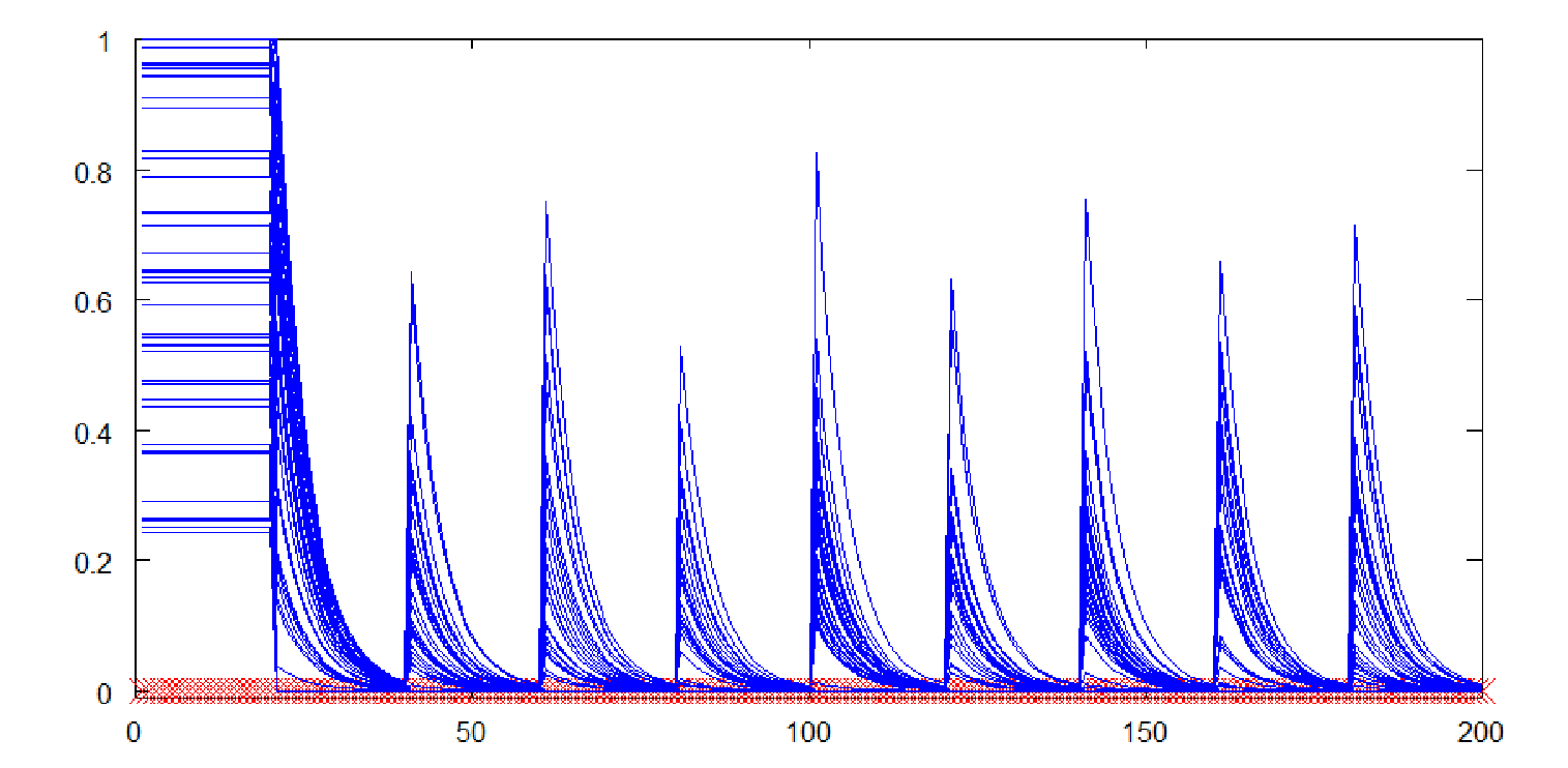
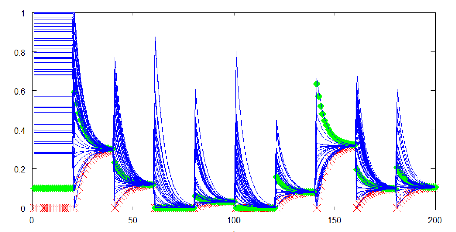
We illustrate Proposition 6.5 in Figure 4, where we let , for all , , and is the random uniform distribution on , and .
Remark 6.3.
As an application of Proposition 6.5, consider the situation when the number of agents goes to infinity. Then, if the fraction of agents in converges to zero, agents become -wise, in the limit, as . Namely, first, the coefficient converges to zero in this case since , so that agents’ expected consensus is indeed as . Moreover, not only do agents’ limiting beliefs converge to in expectation, but agents become indeed -wise in the limit, as the support of the distribution of the -intelligent agents’ initial beliefs is .
As examples of converging to zero, of course, if the number remains constant as , then goes to zero. But even if, for example, grows as in , all agents finally become -wise.
Proposition 6.5 may be restated in the following way; agents’ limiting beliefs, in expectation, are given by , where if . We can then determine the probability that .
Corollary 6.2.
Under the conditions of Proposition 6.5, with probability exactly , we have .
Proof.
The event that the biased agents’ initial beliefs are in is, by the iid property, . ∎
Remark 6.4.
According to the corollary, the probability that is strictly positive but decreasing as the number of biased agents increases. Hence, as becomes large, agents’ limiting beliefs are very likely mixtures of truth and , a value that is different from truth.
Remark 6.5.
We may consider the setup of Proposition 6.5 as a ‘type inference’ problem. What the proposition says and shows is that, since agents adjust their weights based on limiting beliefs, they cannot infer the intelligent agents once a biased non-intelligent agent has guessed truth because agents always reach a consensus in our situation (cf. also Proposition 6.1). Thus, the intelligent agents cannot properly signal their type in this case because all agents’ limiting beliefs are indistinguishable.
Now, consider the exact same situation as in Proposition 6.5, except that agents adjust weights based on initial beliefs, i.e., . In this situation, a sufficient condition for wisdom is that agents find truth sufficiently valuable, i.e., is sufficiently large. In this case, wisdom, in the limit as , obtains almost surely, namely, all that is required is that only the -intelligent agents in are initially true for some topic .
Proposition 6.6.
Let the weight adjustment time point be .
Under the conditions as in Proposition 6.5, if is sufficiently large, then, almost surely, there exists a (time point) such that all agents are -wise for all topics , with .
Proof.
Let be the first time point that (1) only -intelligent agents in happen to know truth, initially, for topic , that is, for all and no ; and, (2) not all agents are -wise for (such that ). Then, weight adjustment at will add to the weights of the -intelligent agents in . If is sufficiently large, after normalization, weights for the non-intelligent agents become arbitrarily small and (arbitrarily close to) uniform for the -intelligent agents. In particular, may be so large that all agents’ beliefs lie in . Since this is a convex set and weight matrices are row-stochastic, beliefs will remain in for all time periods ; hence, agents will be -wise in the limit for topic , and, consequently, also -wise. Since , no more adjustments will occur after time point and all agents become -wise for all topics , with , since their weights are now (sufficiently close to) uniform for the -intelligent agents in . ∎
Example 6.2.
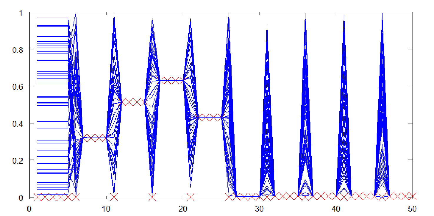
We illustrate Proposition 6.6 in Figure 5, where we let , for all , , and is the random uniform distribution on , and .
Remark 6.6.
To summarize, the intelligent agents in can now correctly signal their type. All that is required is that only -intelligent agents in happen to know truth for some topic, in which case they will receive such a large weight increment that they lead society to -wisdom; then, no more weight adjustments occur because the ‘right guys’ have been identified.
Remark 6.7.
In our current setup, the difference between weight adjustment at vs. at is as follows. While adjusting at leads agents to -wisdom almost surely provided that they find truth sufficiently valuable, that is, is large enough; updating at leads agents to -wisdom provided that biased agents do not know (or, perhaps, ‘guess’) truth for topic . The latter condition is difficult to satisfy if we assume that the number of biased agents becomes large, while the condition of sufficiently large also depends on population size and, in particular, on , the population size of the biased agents. In other words, if , we can specify sufficient conditions for wisdom even under the presence of biased agents, but these are rather challenging.
The case
Now, we consider the same setup as in the last subsection, except that we assume that on its whole domain. In this case, agents continuously adjust their weights to other agents, which is also the rational behavior of an agent who assumes the conditions outlined in Section 4; recall our previous discussion.
We consider a slightly more general situation here than in the last subsection in that we allow each agent to have initial beliefs distributed according to individualized distribution functions, rather than to assume groups with identical distribution functions; the more restrictive setting is then a special case of our generalization. Accordingly, assume that agent ’s initial belief for topic is distributed according to random variable with distribution function for all and all topics , for . We assume that , which gives the probability that agent is within an -radius around truth , does not depend on topic , that is, for all , which means that the probability that agent is truthful is the same across topics. We then have the following proposition.
Proposition 6.7.
Let tolerance be fixed. Assume that agents adjust weights based on initial beliefs, i.e., , and assume that . Then, as , agents’ limiting consensus beliefs on issue are distributed according to
where
with (note that does not depend upon by assumption). In particular, we have
Proof.
Our proof is not rigorous.
Since agents are homogenous with respect to tolerance , they will all jointly increase their weight to a particular agent (or they will jointly not do so). Therefore, as increases, rows of become more and more similar, independent of the initial conditions (if weight matrix is identical in each row, this will propagate to any with , but even if not, rows will become more and more similar by the homogeneity of agents). The weight mass that any particular agent assigns to any particular agent is clearly proportional to (cf. Figure 1) since this value indicates how frequently agent is truthful. Hence, since rows of are (approximately) identical, as becomes large, with each entry being proportional to , limiting beliefs of agents are given by,
where . This completes the proof. ∎
Remark 6.8.
The coefficients have a very intuitive interpretation. Since they indicate how limiting consensus beliefs are formed in terms of initial beliefs, their standard interpretation is that of social influence weights (cf., e.g., Golub and Jackson (2010) [39]). Clearly, in our endogenous weight formation model, with weight sizes dependent upon ‘past performance’, an agent’s social influence is intuitively given by his likelihood of correctly predicting truth.
Example 6.3.
Considering the distribution of limiting consensus beliefs, we note that if two , for , are normally distributed with parameters and , then both as well as are normally distributed; the latter sum has normal distribution with parameters . Hence, if all agents’ initial beliefs are normally distributed, their limiting beliefs are also normally distributed.
Moreover, if there are several ‘types’ or ‘groups’ of agents, , of sizes , where each group has identical and independent initial distribution (within groups), then agents in each group receive about the same weight mass, which is proportional to (see example below) , for , so that if sizes of groups become large, then, by the central limit theorem, is approximately normally distributed. Thus, by our above remark, is also approximately normally distributed. In other words, we would generally expect agents’ limiting beliefs to be normally distributed, in this setup.
Example 6.4.
Consider three groups of agents, with and where the ’s are pairwise mutually disjoint. The first group, which we call experts, has initial beliefs distributed according to , where is fixed (that is, each member in has the given distribution function, and we assume members’ initial beliefs to be independent). The second and third groups are biased. Assume, for illustration, that group two has distribution and group three has . Assume the groups have sizes , and , that is, the group of experts is smallest in size (but still growing in ). Moreover, let, for instance, , and , and let . Then, each expert has of about , members of group two have and members of group three have . Since the ’s must sum to one, we have about for experts, and and for groups two and three, respectively, and where and for . For , this is about , , and , which is also, approximately, the limiting structure of the distribution of as . Hence, in the limit, as , these agents beliefs’ would converge to a consensus that is off by about from truths . More precisely, the agents’ limiting consensus values are distributed according to a normal distribution with mean and variance that converges to zero in ; in particular, variance of limiting consensus values is given by , which is for our example. We plot the (predicted and theoretical) limiting distribution of and a sample histogram from an actual simulation in Figure 6.

In the next proposition, we discuss weight adjustment based on limiting beliefs. We assume that for all non-empty intervals .
Proposition 6.8.
Let tolerance be fixed. Assume that agents adjust weights based on limiting beliefs, i.e., , and assume that . Then, as , agents’ limiting consensus beliefs on issue are distributed according to
In particular, we have
Proof.
Since agents reach a consensus for topics , with , and agents adjust weights based on limiting beliefs, weight matrix entries for all agents converge to . Convergence to is assured since all agents have by assumption such that the probability that agents’ limiting consensus is within an -interval around truth is at least , from which it follows that agents adjust weights infinitely often (which each time entails an increment of and, thus, implies convergence of weight matrix entries to ) with probability . ∎
Remark 6.9.
We see here, again, that adjusting based on limiting beliefs is ‘worse’ than adjusting based on initial beliefs, since limiting beliefs are formed through social interaction and may thus not indicate the inherent ‘intelligence’ of an agent.
To quantify the difference by way of illustration, in Example 6.4, agents’ beliefs would now converge to a consensus, as , that is off from truths by about , which is further away than the value of about given in the situation when agents adjust weights based on initial beliefs. In particular, agents in group , who are very poor at estimating truth, now receive much larger social influence than in the situation where agents adjust based on initial beliefs.
However, qualitatively, the results do not change (by much): in both circumstances, and , agents’ limiting beliefs, under our endogenous weight adjustment process, are given by convex combinations of all agents’ initial beliefs, whereby adjusting based on initial beliefs captures, in the social influence weights , the intelligence of agents while adjusting based on limiting beliefs leads agents to uniform social influence weights .
Now, consider, again, the setup where there are two groups of agents, which we denote by and , respectively; the first groups’ initial beliefs are unbiased while the second groups’ initial beliefs are biased, where we assume that agents within each group have independently and identically distributed initial beliefs. Assume, furthermore, that for all agents .
Corollary 6.3.
Let or and let , the radius within which agents are considered to be truthful, be fixed. Then, if the group of biased agents is ‘large enough’ (e.g., relative to ), agents will not become -wise almost surely as , for any , whereby denotes a random variable that represents the distribution of initial beliefs of any agent from group .
Proof.
By Proposition 6.7 and its proof, if , as (by , we denote the distribution function of an agent from group ; also note that does not depend on by assumption), where and . Thus, if is large enough (relative to ), be may arbitrarily close to such that, in expectation, agents’ limiting consensus belief will be arbitrarily close to , whereby, by assumption, is a biased variable. As , limiting beliefs will converge to almost surely, in this case, by the law of large numbers.
If , Proposition 6.8 leads to the same conclusion. ∎
Remark 6.10.
What Corollary 6.3 shows is that agents may not become infinitely wise under our endogenous weight adjustment process if the group of agents with biased initial beliefs becomes large, as, in this case, this group’s social influence will become arbitrarily large. But the corollary shows more: agents may not become -wise for any , which may be an arbitrarily large interval, depending on the bias of the agents in . In other words, if the number of biased agents is large (relative to the number of intelligent agents), the wisdom that society as a whole can attain is limited by the latter agents’ bias.
6.3 Varying weights on own beliefs
DeMarzo, Vayanos, and Zwiebel (2003) [25] consider a slight generalization of belief updating process (3.1) where agents may place varying weights on their own beliefs such that (3.1) reads as
| (6.4) |
whereby (note that we treat as an exogenous variable). Such a weighting scheme may be empirically plausible, as it has been found (cf., e.g., Mannes (2009) [64]) that people often tend to overweight their own beliefs relative to that of outsiders, probably because individuals have access to their own motivations for beliefs while they do not have such justification for others’ beliefs. This reasoning would imply that is ‘relatively small’. However, as long as weights on others’ beliefs do not drop to zero too quickly, belief updating rule (6.4) leads to the same limiting beliefs as the original DeGroot updating rule (3.1) where , for all , provided that the latter converges; convergence may take sufficiently longer, however. Hence, under these circumstances, all our previous results remain valid. The following proposition is a straightforward generalization of the corresponding theorem, Theorem 1, in DeMarzo, Vayanos, and Zwiebel (2003) [25], which restates the lessons we have just mentioned.
Proposition 6.9.
We list the proof in the appendix.
In all subsequent sections, we only discuss the situations when and , as the other cases may be derived in a manner similar to what we have sketched in this section.
7 Opposition
In this section, we consider the situation when two subsets of agents ‘oppose’ each other. Such opposition may derive, for example, from in-group vs. out-group antagonisms, as is an important concept in psychology and sociology (cf. Brewer (1979) [12], Castano, Yzerbyt, Bourguignon, and Seron (2002) [18], Kitts (2006) [53]) and as has also more recently been taken into account in economics models (cf., in an experimental context, e.g., Charness, Rigotti, and Rustichini (2007) [20], Fehrler and Kosfeld (2013) [32]) and in social network theory (cf. Beasley and Kleinberg (2010) [10]). Prime exemplars of opposition forces can be found in politics (e.g., democrats vs. republicans; opposition parties vs. governing party in charge), for example, or also on a more global societal level (e.g., punks or hippies/counterculture vs. mainstream culture). In the context of (DeGroot-like) opinion dynamics models, opposition has, prominently, been discussed in Eger (2013) [30] (but see also our discussion in Section 2), whose modeling we relate to.
In the model of Eger (2013) [30], there are two types of links between agents. One link type refers to whether agents follow or oppose each other and the other link type denotes the intensity of relationship and is given by a non-negative real number . Belief updating is then performed via the operation
| (7.1) |
whereby the operator is defined via
whereby , where is the identity function (‘agent follows agent ’) and is an opposition function (‘agent opposes/deviates from agent ’). In other words, in this model, agents form their current beliefs by inverting (via ) or not (‘via ’) the past belief signals of others and then taking a weighted arithmetic average, as in standard DeGroot learning, of the so modified (or not) belief signals of their neighbors. As becomes evident, endogenizing this model would require endogenizing two variables, namely, and , a task that is beyond the scope of this section. Therefore, we take as exogenous and keep, as before, as an endogenous variable, formed, in the case that , by reference to an agent’s past performance.1414 14 If , it would make no sense, or be at least problematic, to posit that an agent would increase his intensity of relationship, relating to opposition behavior, in proportion to another agent’s accuracy of predicting truth.
Hence, we consider the following situation. Denote by and the two groups of agents that oppose each other. We posit that is opposition bipartite (cf. Figure 7): for all agents it holds that (analogously for ) and for all agents and it holds that , which simply means that agents within the two groups follow each other whereas agents across the two groups oppose each other.1515 15 This specificiation is not self-evident; intra-group antagonisms, based, e.g., on personalized differences between members of the same group, might plausibly be allowable. Next, we assume that, regarding weight adjustments, members of both groups ignore members of the other group (a sin or bias of omission), taking into account only members of their own group, that is,
| (7.2) |
where denotes the group of agent , which is either or ; for simplicity, assume , here and in the remainder of this section. Finally, we assume that agents of group initially assign uniform intensity of relationship to each member of group and members of group do analogously, assigning , where and are positive constants. We also assume that these levels stay fixed over topics, that is, whenever . When , as said, we let weights be formed according to (7.2). Finally, we always assume that weight matrices are row-stochastic. We now discuss the so specified model, with endogenous weight (or intensity) formation for at least a subset of agents, in the following example. For opposition function , we let be soft opposition on (see Eger (2013) [30] for details) with the functional form . We first outline the following proposition from Eger (2013) [30], which gives conditions for convergence of , where we omit, here and in the following, reference to topics for notational convenience.
Proposition 7.1.
Let be soft opposition on . Then, is affine-linear with representation . Then, if is opposition bipartite, is an eigenvalue of . If is the only eigenvalue of on the unit circle and if has algebraic multiplicity of , then for some polarization opinion vector (that depends on ) and all initial opinion vectors .
In the proposition, a polarization opinion (or belief) vector is any vector consisting of two beliefs such that and . For our specification of , this would mean that . Hence, the proposition says that if is soft opposition, then is representable by a matrix , and if in addition is opposition bipartite (as we assume), then convergence of depends on the eigenvalues of . In the following example, we will make reference to the proposition.
Example 7.1.
Let and with . Before (partly) endogenizing , assume first that and have the following form,
| (7.3) |
where , , , , and , ; matrices and are of size , and of size , etc. Hence, agents in follow each other, assigning weight to each other, and agents in assign weight to each other; across the two sets, agents oppose each other, with weights and , respectively, as already indicated above. Moreover, for simplicity, as the given specification posits, we assume that weights are uniform within groups and opposition weights are also uniformly distributed. Since, as Proposition 7.1 tells, the so defined allows an (affine-)linear representation, this is given by, in this setup,
| (7.4) |
as one can verify (cf. Eger (2013) [30]). Furthermore, if converges to a polarization vector (e.g., under the conditions of Proposition 7.1), then the one limiting belief is given by and the other is given by , where is the unique eigenvector of satisfying and corresponding to eigenvalue of (cf. Eger (2013) [30], Remark 6.4). The vector is then a (generalized) social influence vector (cf. the concept of eigenvector centrality, e.g., Bonacich (1972) [11]), with denoting the social influence (proper) of agent and his group membership. Since, by our specification of , agents in group must have the same social influence (by homogeneity of these agents due to the uniform weight structure) as well as agents in group , we must accordingly have that for some . Then, (or ) measures social influence of members of group and accordingly for . Hence, from , we find (1) , (2) , and (3) (from the unit condition on ). From this, it follows that
| (7.5) |
The case of may serve as an illustration. Computing the comparative statics of with respect to and , we first find that since , it holds that . Hence, and then,
such that an increase in leads to an increase in the absolute value of , as we would expect — if the weight that members of group place upon each other increases, their social influence, measured in absolute value, increases. Moreover, also increases in — the more members of group want to disassociate from members of group , the more does group ’s social influence increase, in absolute value. We exemplify in Figure 8 (left).
Hence, under our current assumptions, limiting polarization beliefs of agents are given by and , respectively. Let us, for the moment, assume that all agents are -intelligent with , that is, all agents precisely receive truths for topics, as initial beliefs. Then, limiting beliefs are, thus,
respectively, where closed-form solutions of and are given in Equation (7.5). In Figure 8 (right), we plot, for and fixed, the coefficient of limiting beliefs (and its negative, as coefficient of the other limiting belief), as a function of (and, hence, also of since ); note that this coefficient denotes the ‘scaling’ of truth in the limiting beliefs, whence, if it is equal to , (some) agents exactly reach truth. We observe the following: if is very low (compared with ), i.e., agents in group care little about agents in group (at least relatively) — that is, opposition from to is (relatively) low — then is very close to , which means that agents in group have limiting beliefs very close to truth, while agents in group hold limiting beliefs that are very close to , the ‘opposite’ of truth. As increases, becomes smaller, approaching zero as . In other words, if opposition ‘force’ is equal between groups and — in the sense that — then both groups reach limiting beliefs of zero, no matter what truth is. As group begins to oppose group more heavily than opposes , that is, , group goes further away from truth, toward opposite levels of truth in that becomes negative, while group begins to approach truth.
Now, concerning the question whether the conditions on the eigenvalues of matrix , stated in Proposition 7.1, are satisfied — that is, do agents in fact converge to a polarization? — we mention that exactly determining the spectrum of is difficult in the current situation, for general and , and . For and arbitrary (and, by symmetry hence also for and arbitrary), we find, in the appendix, that has exactly one eigenvalue, namely , on the unit circle and whose algebraic multiplicity is . Thus, in this case, by Proposition 7.1, beliefs under indeed converge to a polarization, as we have sketched it, and limiting beliefs have the indicated form. We strongly suspect that this is true for arbitrary and , but leave the derivation open.
Finally, when would we expect to have the form (7.3), taking the form of as exogenous? The structure of holds, for instance, when has the form indicated in (7.3), agents adjust weights (to members of their own group) based on initial beliefs, , and, e.g., (agents’ initial beliefs are exactly ); then all have the form as given in (7.3). Form (7.3) also arises, in the limit, as becomes large, when and initial beliefs are stochastically centered around truth and each agent has the same variance (namely, agents then tend to assign uniform weights to those they take into consideration in adjusting weights; uniform weights for outgroup members have been assumed exogenous by us, anyways). In fact, the simulations shown in Figure 9, for the latter case, show good agreement with the analytical predictions for the situation when all agents are -intelligent, for , even for small , indicating that has a form close to (7.3) quickly, when agents are stochastically intelligent with identical variances.
Remark 7.1.
In Example 7.1, we have outlined conditions under which we expect, due to polarization, at most one group of agents to become wise for topics. The conditions that we have highlighted — e.g., -intelligence, for , or initial beliefs stochastically centered around truth whereby all agents have identical variances — might appear quite special. We believe that similar polarization results hold for much more general conditions, but those outlined have the benefit of being analytically tractable more easily while still indicating results, as we think, of a general nature.
Remark 7.2.
To summarize the importance of results indicated in Example 7.1, note that in this section, agents have been influenced by two ‘polar’ forces. On the one hand, they were attracted by truth by their adherence to principles that potentially lead them closer to truth — e.g., weight adjustment to those agents in their in-group that have been truthful in the past. On the other hand, agents had — exogenously — specified antagonisms to members of another group (a sin or bias of commission), their outgroup, which drew them toward beliefs that are different from those held by their adversaries. The message from Example 7.1 is clear in this context: the group that has (relatively) stronger incentives to disassociate from negative referents tendentially will drift away from truth considerably, while the group with (relatively) weaker such incentives may still become wise (under appropriate initial conditions on beliefs), which is an intuitive result since, for the former group, disassociation seems to be (relatively) more critical than truth.
8 Conformity
Buechel, Hellmann, and Klößner (2013) [15] and Buechel, Hellmann, and Klößner (2012) [14]1616 16 Henceforth, we only relate to the more recent version of their paper, unless the difference becomes important. study a DeGroot-like opinion dynamics model under conformity, that is, where individuals are not only informationally socially influenced by others but also normatively in that they are motivated to state opinions that tend to fit the group norm, possibly, in order to get “utility gain[s] by simply making the same choice as one’s reference group” (cf. Zafar 2011 [76], p. 774). A classical example of such conforming behavior is documented in the famous study of Asch (1955) [6] where subjects wrongly judged the length of a stick after some other, supposedly neutral, participants had given the same wrong judgment. More examples and relevant theoretical and empirical literature, e.g., Deutsch and Gerard (1955) [26], Jones (1984) [49], etc., on conforming behavior among human subjects are directly provided in Buechel, Hellmann, and Klößner (2013) [15]. As we have indicated in the introduction, we may perceive of conformity to a reference opinion, in our context, as a bias toward the beliefs of one’s reference group.
Mathematically, agents in the named model update their beliefs informationally according to the following rule,
| (8.1) |
where denotes the vector of stated opinions or beliefs (whose formation, as assumed, underlies normative social pressure, as we indicate below), denotes the vector of true beliefs, is the social network (or, ‘learning matrix’) as in the standard DeGroot model, and denotes its diagonal. Updating rule (8.1) says that agents form their current beliefs by taking a weighted arithmetic average of their past true beliefs and others’ stated beliefs. Then, as concerns normative social influence, agents are assumed to choose stated beliefs by reference to the utility maximization problem
| (8.2) |
whereby the term represents an agent’s preference for honesty (misrepresenting true opinions may cause cognitive discomfort, cf. Festinger (1957) [33]) and the term represents preference for conforming to a reference opinion . The parameter displays the relative importance of the preference for conformity in relation to the preference for honesty. If , then agents have preference for counter-conformity in that their reference group serves as a negative referent. Now, consider that at the end of each (opinion updating) round , agents play a normal form game . Let and let where is an matrix that indicates how reference opinions are formed from stated opinions; we assume that for all such that agents do not take into account their own stated opinion in reference opinion formation1717 17 They know better anyway, by knowledge of their true opinions. and we also assume that is row-stochastic. The next proposition says that the normal form game has a unique Nash equilibrium.
Proposition 8.1.
Denote by the diagonal matrix with . Then the normal form game , for , has a unique Nash equilibrium, which is given by
We prove Proposition 8.1 in the appendix. The proposition is a (straightforward) extension of the corresponding proposition, Proposition 1, in Buechel, Hellmann, and Klößner (2012) [14] in that they choose the particular with (). In the revised version of their paper, the named authors also specify an iterative process that explains how agents reach the Nash equilibrium but we omit the recapitulation of this idea, because it is rather technical and does not provide further insight at this point.
Hence, simply assuming that agents play the Nash equilibrium at the end of each period (such that, for , and are available), beliefs evolve according to, combining (8.1) with ,
where
| (8.3) |
and where we also index matrices by topic indices. As becomes obvious, this model has now many variables that can potentially be endogenized, namely, , , which summarizes the conformity parameters, and , which summarizes how agents form reference opinions. In the following, we take as exogenously given and constant across topics; the elements may then be perceived as ‘personality traits’ of individuals. For , we assume the same endogenous weight formation as before, where weight increments depend upon past performance. The matrix , we take as arbitrary exogenous variable first, satisfying row-stochasticity and as above, and specialize then in the examples.
Our first proposition paths the way for a convergence result in our situation. It says that the property of having a positive column propagates from to if no agent is counter-conforming.
Proposition 8.2.
Let be arbitrary. Let for all such that agents never counter-conform. Then, if has a positive column, then so does .
Proof.
By the proof of Proposition 8.1, given in the appendix, the inverse of always exists (as long as , which we assume throughout) and is given by . Since and since is assumed to be row-stochastic, the latter sum is a sum of non-negative matrices and therefore, the infinite sum yields a matrix with non-negative entries. Moreover, since for any arbitrary matrix , all diagonals of are hence strictly positive ( has strictly positive diagonals and the remaining summands are all non-negative). Moreover, since is a diagonal matrix with each entry ,
accordingly also has diagonal entries that are all strictly positive. Next, since has a strictly positive column by assumption, has a strictly positive column , except for element of that column, which is zero. Hence, multiplying, , a non-negative matrix by assumption, with results in a matrix that also has a strictly positive column , except possibly for its diagonal. But since has a positive entry (since column of is positive by assumption),
has a positive column . The latter matrix is, by definition (Eq. 8.3), precisely the matrix . ∎
As a corollary, we have our first convergence (to consensus) result, which provides both an alternative to the convergence result provided in Buechel, Hellmann, and Klößner (2013) [15], and a generalization as well as a strengthening. It is more general since it considers arbitrary rather than the peculiar choice that the named authors consider. It provides an alternative since it says that conformity and a positive column of are sufficient conditions for convergence, while the proposition in Buechel, Hellmann, and Klößner (2013) [15] states that conformity and a positive diagonal of are sufficient conditions for convergence. Finally, it is a strengthening because it states convergence to consensus rather than merely convergence. Before proving the theorem, we need the following lemma which says that the rows of sum to and which we prove in the appendix.
Lemma 8.1.
Corollary 8.1.
Let be arbitrary. Assume that for all . Then, if has a positive column, then induces a consensus.
Proof.
It might be worthwhile, in future considerations, to study in more depth which properties inherits from , and under which conditions. As mentioned, Buechel, Hellmann, and Klößner (2013) [15] demonstrate that inherits a positive diagonal from (under their particular choice of and under conformity) as well as the general social network structure (see their discussion in their Section 4), while we show that the property of positive columns also propagates, for arbitrary .
For now, we contend ourselves with the fact that Corollary 8.1 implies that, as in the standard DeGroot model, agents almost always reach a consensus — that is, for almost all topics — even under conformity (), under very mild conditions.
Proposition 8.3.
Let , agents’ tolerance, be fixed. Let (resp. ). Let . As in Proposition 6.1, let be the earliest time point that some agent is -intelligent (resp. -wise) for topic . Then, under the conformity model presented above, with for all , (a) agents reach a consensus for all topics with , independent of their initial beliefs. (b) For topics , agents’ reaching a consensus depends on and on to as well as on to .
Proof.
(a) As in the corresponding proof of Proposition 6.1, has a positive column and so do, in general, have all matrices , for . Hence, by Corollary 8.1, agents reach a consensus for topics , for , under the conformity model, as long as for all . (b) Of course, whether or not agents reach a consensus for to depends on the parameters of the model. ∎
As mentioned before, if there exist agents whose initial beliefs have positive probability of lying within an -interval around truths, then , as defined in Proposition 8.3, is a finite number almost surely. For standard parametrizations (e.g., all agents have positive probability of being truthful, for all topics), is very low — typically — with probability that goes to in , population size (cf. Remark 6.2).
Example 8.1.
If agents are counter-conforming, Proposition 8.3 may be false in that beliefs may even diverge, rather than lead to a consensus. Consider, for instance,
which would be the resulting weight matrix if and agent ’s and ’s initial beliefs were in an -radius around truth, for the first time, for topic . For convenience, assume that
where . Then, sample belief dynamics for this setting are sketched in Figure 10. As the graphs illustrate, under counter-conformity, agents may want to diassociate from others in a manner strong enough to induce divergence.


Next, we discuss social influence of agents as a function of conformity parameters and the structure of . In particular, we show that even agents with an ‘empty record of past successes’ can be influential in the endogenous conformity model if conformity parameters and matrix are appropriately specified.
Proposition 8.4.
Let for all . Assume that is strictly positive on all off-diagonal entries. Then, if has at least two positive columns, is strictly positive everywhere.
Proof.
Again, is
We have is strictly positive in each entry since is positive on all off-diagonals and since , whence is positive on all off-diagonals and note that has positive diagonals; the remaining terms , for , are non-negative. Hence, also entrywise, since the diagonals of are positive. Hence, since has at least two positive columns, is also positive and then also . ∎
Remark 8.1.
Thus, if is strictly positive in each entry (other than the diagonals) and all agents are (strictly) conforming and has at least two positive columns, then is strictly positive in each entry. This means that is strictly positive in each entry, for all powers . This also means that , which exists for a row-stochastic that is strongly connected and aperiodic (as an with strictly positive entries is), is positive in each entry. But this means that, under conformity, if agents form their reference opinions , to which they strive to conform, with respect to all other agents (that is, is strictly positive, except for the diagonals), then each agent has strictly positive social influence on the limiting beliefs, even if has never been truthful in the past. The amount of influence (even non-truthful) agents have on limiting beliefs depends then both on past performance and on the conformity parameters . We illustrate in the next example.
Example 8.2.
Assume the following situation. There are agents and has the form
Such a may arise, for instance, for large , when and when agents and have initial beliefs centered around truth, with identical variances, and agent has never been truthful, for instance, because , for all . Assume that
which means that everyone weighs everyone else uniformly in forming reference opinions, and assume that is constant across topics. Finally, let and , where . Consider the social influence of agents — that is, their influence on limiting beliefs as a function of initial beliefs. Since agents and are identical, they must have the same social influence, which we denote by , and let agent have influence , such that . In the appendix, we show that has the form
Computing the comparative statics with respect to and , we find
Thus, influence of agent decreases in own conformity, , and increases in conformity of the stochastically intelligent agents, . Moreover, we find
such that agent , who has zero probability of knowing truth, may have arbitrarily large social influence on limiting beliefs, as long as agents and exhibit arbitrarily large conformity, and agent ’s social influence may also vanish, as his own conformity becomes arbitrarily large. In Figure 11, we plot as a function of (for fixed levels of ) and (for fixed levels of ).
Note that this result, namely, that an agent with zero probability of being truthful may become arbitrarily influential, could not have been possible in the standard model with endogenous weight formation as we have sketched, since such an agent’s social influence would always be zero (or converge to zero) by the results developed in Section 6, as becomes large. This result would also not have been possible had there been only one positive column of matrix (and the others all zero) since in this case the corresponding agent, even if he were excessively conforming and would thus state an opinion arbitrarily close to that of his reference group, would both ignore his own stated opinion (because he knows his true opinion) and that of others (because all other columns are zero, by assumption) such that the agent corresponding to the positive column would always have social influence of . In other words, we require at least two conforming intelligent agents in order for a non-intelligent to be able to become influential, under our current model specification.
To summarize, our current example shows that if conformity parameters are ‘adequately’ specified, an agent with zero probability of being close to truth may become arbitrarily influential, which, again, means that society may be arbitrarily far off from truth in our setup. In particular, under conformity, society may be drawn away from truth by agents without any past successes.1818 18 Which might be an explanation of why even ‘blatantly’ and repetitively false propaganda may work.
But, of course, a crucial aspect in the current example has also been matrix , which determines how agents form reference opinions, and which agents a particular agent strives to conform to, and which we have assumed strictly positive. Of course, it might not be implausible to assume that depends, in particular, on past performance. This is our final example.
Example 8.3.
Let for and let such that is formed in an analogous way as .1919 19 As mentioned, this is the specification discussed in Buechel, Hellmann, and Klößner (2013) [15]. In particular, in this setup, agents want to conform to those who have performed well in the past. Assume that there are two types of agents, whereby one type has initial beliefs centered around truth as in (6.1) and the other type has zero probability of ever being truthful, for all and all where is the set of agents of type two, and by we denote the set of agents of type one. Then, if and as becomes large, has the structure where in each row , for ( is a normalization constant) and for , by the results developed in Section 6, and where is the variance of agent ’s initial belief. The informational social influence of agent is then also given by, roughly, , for , and , for , respectively. Moreover, the combined informational as well as normative social influence of agents is given by
for agents and for agents . These results follow directly from Theorem 1 and Corollary 1 given in Buechel, Hellmann, and Klößner (2013) [15], which precisely state that closed and strongly connected groups (which is, at least for large ) have social influence as given and the ‘rest of the world’, which group forms, has .
This example shows that if follows the structure of , then, unlike in the previous example where was uniform (or at least strictly positive on the off-diagonals), agents that never know truth cannot be influential. It moreover shows that social influence decreases in conformity (for the agents in ), as we have already observed in the previous example.
Investigating social influence in the general case, for arbitrary , and , would be highly interesting, as it indicates to which degree agents who are never truthful can still be influential, and scope for future work.2020 20 Proposition 8.4 is an important step in this direction already, since it says that if is strictly positive on all off-diagonals, is strictly positive in all diagonals, and has two positive columns, then all agents are influential.
9 Homophily
In this section, we extend the standard endogenous weight adjustment opinion dynamics model discussed in Section 6 by introduction of the concept of homophily, according to which, as McPherson, Smith-Lovin, and Cook (2001) [65] phrase it, ‘similarity breeds connection’, and which is a majorly accepted standard concept in modern socio-economic research. In the opinion dynamics literature, homophily has been modeled by positing that weights (social ties) between any two agents are functionally dependent on the agents’ current belief distance (cf. the Hegselmann and Krause models, Deffuant, Neau, Amblard, and Weisbuch (2000) [23], Pan (2010) [67], etc.), that is, agents with more similar current beliefs place greater (current) weight upon each other. Opinion updating is then performed as in standard DeGroot learning, via weighted averages of peers’ past beliefs, where the weights are now endogenously formed by the homophily principle. As indicated in the introduction, we think of homophily, in our context, as arising from biased reasoning, where individuals overrate beliefs that are similar to their own (cf. Kunda (1990) [55]).
In the Hegselmann and Krause models, to which we relate, agents set time-varying weights according to the following rule,2121 21 Note that, thus far, we have assumed weights to be only varying across topics and not in addition across discussion rounds (time) within a given topic.
where denotes the set of agents within an -radius, for , around agent ’s belief at time , that is, , and where is an external parameter. One plausible integration of this setup in our framework is to let agents increment weights to other agents whenever distance between their current beliefs is sufficiently small, that is,2222 22 Otherwise, if weights were not incremented but rather set in an ‘absolute manner’, the continuity of weight relationships across topics could not be maintained.,2323 23 After each round , we renormalize weights in order for them to satisfy the row-stochasticity condition.
| (9.1) |
Then, after truth is revealed, agents again adjust weights according to the ‘truth related’ principles outlined in Section 3. In particular, we would now have,
| (9.2) |
for all , where we need to consider, for next topic’s initial weights, the limit, as time goes to infinity, of the time-varying weights for the previous topic, since weights are now also adjusted within topic periods. Note that, here, we also subscript — the radius within which weights are adjusted — and — the weight increment — by and , respectively, depending on whether we relate to adjusting/incrementing based on truth or based on homophily.
Also observe that (9.2) is well-defined only if exists, which we naïvely assume in the following but the formal proof of which we leave open. It is worthwhile mentioning that adjusting weights based on truth may microeconomically be justified precisely as we did in Section 4 — namely, it may follow from the tenet that agents have disutility from not knowing truth, whence, by incrementing weights to agents who have been truthful in the past, they increase their likelihood of eventually becoming close to truth, provided that the assumptions they make (bona fides, etc.) are satisfied. In contrast, we offer no explicit microeconomic foundation --- that is, based on utility functions and their explicit maximization --- here of why agents would increment weights to other agents based on the homophily relation, taking this behavior simply as a form of (exogenous) bias. Moreover, similar as in the opposition model, it is appropriate, in the current setting, to think of agents as motivated by two contrarian forces --- truth and homophily ---2424 24 Note that in the opposition model, the two forces were an agent’s ingroup and his outgroup. which may possibly act to the ‘same ends’, but which we generally think of as of antipodal origin and direction.
Concerning updating of beliefs, beliefs evolve according to
| (9.3) |
as outlined in Section 3, with the addition that we now let weights vary within discussion periods. Due to the slightly greater complexity involved in belief dynamics, we summarize the belief evolution process in the below schematic form.
Providing general results for the belief dynamics process currently under consideration is not so easy since weights do not only vary by time now, but, in particular, by the current belief state vector . Lorenz (2005) [59] gives convergence results for this general setup, which we list in Appendix A, whose assumptions, however, do not apply to our situation. As a first illustration, still, we show that, unlike in the standard model and under conformity, even after some agent has been truthful for a topic , agents need not converge to a consensus, but may hold distinct limiting beliefs about ; whether consensus obtains or not may depend on the relative sizes of , which we may think of as ‘importance of truth’, versus , which we may think of as ‘importance of homophily’.
Example 9.1.
Let there be agents. Assume that is the identity matrix. Moreover, let and assume that agent receives initial signal and that agents , and are not within an -radius around truth, for topic . Finally, assume that any two agents’ initial beliefs and are at least a distance of away from each other for topic so that homophily plays no role for topic . Then, at the beginning of topic , agents adjust weights based on truth such that looks as follows
Assume that initial beliefs of agents for topic are and , whereby initial beliefs of agents and , on the one hand, and and , on the other hand, are at a distance of at least . This specification means that agents and , on the one hand, and and , on the other, form distinct ‘homophily clusters’, at least at time , for topic . In Figure 12, we sketch belief dynamics for topic for different values of , with and fixed. We see that, unlike in the standard DeGroot learning case in this setup (and also in the conformity model) and as already indicated, agents do not necessarily reach a consensus. If homophily is ‘too strong’, that is, is ‘too large’, agents polarize in this setting. As homophily becomes weaker, that is, becomes smaller, the beliefs of agents and move closer to the beliefs of agents and , the former of which has been truthful for topic . As falls below a certain threshold, the agents reach a consensus.

To sketch one (simple) result of a general nature, here, however, consider, similarly as before, the situation when there are two groups and of agents, whereby agents in are -intelligent, for a fixed , and agents in have initial beliefs with , that is, agents in have initial beliefs such that the probability that they ‘correspond to’ truth is zero. In the next proposition, we show that all agents may become -wise, even if , in this situation provided that agents value truth ‘sufficiently much’ and value relations based on homophily sufficiently little. This result is not entirely trivial because, for instance, for our opposition model, arbitrarily small ‘opposition force’ could induce (at least some) agents to not converge to truth. The result says that homophily does not always need to interfere with wisdom.
Proposition 9.1.
Let , , and topic be fixed, for .2525 25 For topic , there are no weight adjustments based on truth, so we exclude this situation. Then there exist large enough and small enough such that all agents become -wise for .2626 26 Of course, if were zero, any positive would satisfy the conditions of the proposition. In our setup, we assume, however, that homophily always plays a role, that is, for all ‘homophily increments’ .
Proof.
Since the agents in are -intelligent, with , all agents adjust weights for these agents based on truth. By choosing large enough and small enough (but positive), it can be ensured that beliefs , for all , are in the (open) -interval around truth (the weights for the -intelligent agents may become arbitrarily close to uniform provided is large enough and is small enough and the weights for the agents in may become arbitrarily close to zero). Since is row-stochastic, for every , and since the (open) interval of radius around truth is a convex set, all belief vectors , for , lie, component-wise, in . ∎
Remark 9.1.
In the last proposition, and may depend upon the topic (e.g., in particular on the distribution of initial beliefs for this topic). If we let, and ,2727 27 This would require to ensure that the so defined is strictly positive (rather than zero) and that . then for this choice of and , all agents will be -wise for all topics , for .
Example 9.2.
We illustrate Proposition 9.1 in Figure 13, where we sketch belief dynamics for a sequence of topics for fixed parametrizations and various choices of and . In the figure, we simulate belief dynamics across topics for agents, where agents are -intelligent and agents have initial distribution of beliefs such that their initial beliefs are never in an interval around truth; for the sake of concreteness, we let , for all , , , and for the agents in , we let their initial beliefs be distributed according to the random uniform distribution on the interval .
The graphs illustrate, first, that truth attracts all agents since even the beliefs of the agents in move in the direction of truth, as time progresses. However, as long as preference for homophily is not small enough and preference for truth is not large enough, the agents in do not become -wise for topics. The graphs also illustrate the clustering of beliefs due to the homophily relationship, a circumstance well-known from the classical Hegselmann-Krause models.


Remark 9.2.
The graphs in Figure 13 show much analogy with results of the original opinion dynamics model ‘under homophily’ as developed in the work of Hegselmann and Krause, on which our current modeling is based (recall that the difference is that we increment weights in case two agents’ beliefs are similar, while they set weights uniformly in this case, and that we in addition introduce truth as an influential factor). In particular, in the graphs, we find that
- •
the opinion dynamics process always converges, and that
- •
agents (or, rather, their beliefs) cluster into subgroups in which agents reach a consensus.
Proving these apparently generally true observations is beyond the scope of our investigation here, and we leave it for future consideration.2828 28 See Krause (2000) [54] for a starting point on how to prove the results in question.
We close this section by presenting simulations on the role of the truth related radius and the homophily related radius , respectively. Concerning , we find in Figure 14 that a smaller (that is, based on homophily, agents trust/listen to only those with very similar beliefs) tends to produce a larger degree of fragmentation of limiting belief spectra while larger (that is, based on homophily, agents even trust/listen to agents with rather distinct beliefs) tends to promote global agreement among agents. Interestingly, smaller also leads agents closer to truth (since the homophily relation applies to fewer agents). Concerning , in Figure 15, we find that, overall, an increase in increases the average distance of limiting beliefs to truth since also beliefs that are remote from truth are taken into consideration in link weight adjustment.


In sum, in this section, we have shown that, under the ‘homophily bias’ and under the presence of agents with biased initial beliefs, agents need neither become wise nor reach a consensus. If the homophily relation is sufficiently ‘weak’, wisdom may obtain (Proposition 9.1), but if it sufficiently ‘strong’, agents’ beliefs will generally cluster into distinct regions of the belief spectrum. As in the conformity model (and also as under opposition), even agents with zero probability of being close to truth may influence others.
10 Conclusion
As Acemoglu and Ozdaglar (2011) [3], and many others, point out, the importance of the beliefs we hold cannot be overstated. For example, the demand for a product depends on consumers’ opinions and beliefs about the quality of that product and majority opinions determine the political agenda. Thus, beliefs also shape (our) behavior in that they lead us to buy certain products and reject others or in that they are causal factors for the implementation of laws and policies. On a more abstract level, the set of norms and beliefs we hold determine, in the end, who we are and substantiate our cultural foundations. In modern microeconomic research, beliefs and opinions are thought to originate from social learning processes whereby individuals are situated in a network of peers and update their opinions, e.g., via communication with others. Rejecting the hypothesis that individuals are fully rational, much recent research has assumed that people learn from others via simple ‘rules of thumb’, simply averaging peers’ past beliefs to arrive at new beliefs. Then, given that there exist ‘true states’ for the issues that individuals hold beliefs about, a natural question to ask is whether such agents, who commit the bias of not properly accounting for the repetition of information they hear, can, in fact, still learn these true states and, thus, become collectively ‘wise’ (cf. Surowiecki (2004) [69]), successfully aggregating dispersed information.
In the current work, we have studied belief dynamics under an endogenous network formation process. In particular, we have assumed that agents strengthen their ties to other agents based on the criterion of ‘past performance’ such that agents increment their trust weights to whoever has been ‘close enough’ to truth for a current topic. We have, moreover, assumed that agents are multiply biased in that they are not only susceptible to persuasion bias — the simplifying DeGroot learning rule — but also have biased initial beliefs (the possibly non-social, ‘intelligence-based’ substrate of beliefs), and commit several other sins of reasoning, such as being biased toward members of their in-group and motivated to disassociate from members of their out-group, being motivated to conform with the beliefs of their reference group, or overrating beliefs that are close to their own. Our goal has been to outline situations under which collective failure (or at least, ‘failure of wisdom’) can obtain, even though the potential for wisdom — dispersed correct information — is assured. Thus, our work was also in part targeted at the recent ‘optimism’ concerning biased (‘naïve’) learning in social networks and crowd wisdom (e.g., Golub and Jackson (2010) [39]), which has also been challenged by experimental research (cf., e.g., Lorenz, Rauhut, Schweitzer, and Helbing (2011) [62]).
As to our results, under the standard DeGroot learning model, we have seen that wisdom can fail if there are sufficiently many agents with biased initial beliefs such that they, still, have positive probability of being close to truth. The intuition behind this result is that even if the biased agents have small, but positive, probability of ‘guessing’ truth, then, if they are sufficiently many — such that many of them will still be close to truth — the biased agents can, in total, receive large enough weight mass from all agents, whence they may become arbitrarily socially influential, leading all of society to the expected value of a biased variable, away from truth. This result may be thought of as based on the bona fides bias, which says that agents do not give up the assumption that their own (initial) beliefs are unbiased and that others’ beliefs share this property with their own, even despite potential collective failure, from which it may be motivated that agents continuously apply their trust weight incrementing rule (to all agents). In the conformity model, wisdom may fail even when the biased agents have zero probability of being close to truth and when their number is small, provided that the unbiased agents are sufficiently conforming. We might take this as an argument for why even ‘blatantly’ and repetitively false propaganda could work. A necessary condition for this result is that agents want to conform to reference groups including even biased and completely unknowing agents (which might be justified on grounds/biases such as truth-unrelated prominence, e.g., due to political power or popularity). In the opposition model, wisdom can fail even if all agents’ initial beliefs are unbiased and, in addition, arbitrarily close to truth, merely as a consequence of agents being attracted by contrarian forces — their in-groups, on the one hand, which attract them toward truth, and their out-groups, on the other, from which they want to disassociate. In the homophily model, wisdom can fail because agents are, again, influenced by antagonistic forces — truth, on the one hand, and agents with similar beliefs, on the other. Hence, biased agents’ beliefs may cluster, if they form a homogenous group, and unbiased agents’ beliefs may also cluster, so that some agents would become wise and others not.
Concerning future research directions within our context, of course, endogenizing several (more) of the parameters of the DeGroot learning models that we have discussed might be of interest. In the current work, we have solely endogenized the social network, without explaining, for example, where in-group/out-group antagonisms actually come from or how conformity may develop and how reference groups evolve. The endogenizing of such parameters would plausibly require psychological and socio-economic motivations that are independent of the criterion of ‘past performance’. Moreover, in our model, we have generally assumed that agents are homogenous with respect to many dimensions of attributes such as their truth tolerances , trust weight increments , etc., and a heterogenous setup may provide further insight. Finally, introducing strategic agents (cf., e.g., Anderlini, Gerardi and Lagunoff (2012) [5]), that potentially have incentives to deliberatively mislead others, might be a promising research direction to incorporate in our general setup of social learning and collective wisdom/failure.
Appendix A Proofs
Standard model
Lemma A.1.
If matrix has identical rows with row sum , then for any .
Proof.
Follows by induction. ∎
Wisdom of crowds under initial beliefs centered around truth
The following are results from Golub and Jackson (2010) [39]. They state conditions under which a growing population, parametrized by its size , converges to truth under the assumption that agents receive initial belief signals that are centered around (as in (6.1)). The statement of the below results is that agents become (-)wise (for any ) if and only if the influence of the most influential agent converges to zero as increases, whereby an agent’s influence is given by his social influence, as we have discussed above and as we define below. In undirected networks ( for all ) with uniform weights, this condition is tantamount to all agents’ relative degrees (the number of links they have to other agents divided by the total number of links in the network) converging to zero as becomes large. Hence, in this setup, an obstacle to wisdom would be the circumstance when each agent who newly enters society assigns, e.g., a constant fraction of his links to a particular agent, who would then become excessively influential.
Remark A.1.
If a social network induces a consensus, then limiting beliefs can be represented as , for a non-negative vector with which we call the social influence vector and agent ’s influence. The influence vector is given as the unique normalized unit-vector which satisfies (i.e., is the normalized unit-eigenvector of corresponding to the eigenvalue ).
Now, as in Golub and Jackson (2010) [39], we parametrize social networks by their population size , which we denote by ; we also parametrize other quantities such as limiting beliefs of a set of agents by population size (here and in the following, we omit reference to topics for notational convenience). Moreover, we denote a society by the sequence . We restate the following lemma and the proposition from Golub and Jackson (2010) [39], which they list as Lemma 1 and Proposition 2.
Lemma A.2 (A law of large numbers).
If is any sequence of influence vectors, then
(where convergence is in probability or almost surely) if and only if , where we assume, without loss of generality, that .
Proposition A.1.
If is a sequence of networks, each inducing a consensus, then the underlying agents become (-)wise (for any ) as if and only if the associated influence vectors are such that as .
We now argue informally that the proposition entails convergence to truth in the situation where agents’ initial beliefs are centered around truth as in (6.1) and in our setup of endogenous weight formation.2929 29 We assume that is so large that each network always induces a consensus. Note that, if agents are stochastically intelligent, a consensus is reached quickly (and increasingly fast in the number of agents ), by the results developed in Section 6. Namely, we first argue that an agent’s influence is directly inversely proportional to his variance . Although a proof thereof would require technical sophistication, the claim appears very intuitive since influence captures weight mass assigned to an agent by other agents (in addition to these agents’ influence; cf. DeMarzo, Vayanos and Zwiebel (2003) [25]) and, in our setup, the weight mass that an agent receives is directly inversely proportional to his variance (more intelligent agents receive weight increases more often). Next, consider networks where, for all , agents’ variances satisfy for some lower bound .3030 30 Should there be no lower bound on the most intelligent agent’s variance, then this agent may become excessively influential but his initial beliefs also become arbitrarily accurate, so that society becomes (-)wise simply because one agent is arbitrarily well-informed. Then, as , the influence of the most influential agent certainly goes to zero since the number of agents increases (all of which are influential in the sense that they receive weight mass from others) while the expected weight mass that the most influential agent receives is bounded.
Varying weights on own beliefs
Proof of Proposition 6.9.
Since converges for all initial belief vectors , there exists a matrix such that . To prove the proposition, show that converges to as , whereby and where according to (6.4). Proceed exactly as in DeMarzo, Vayanos, and Zwiebel (2003) [25].
Define the random variable to be equal to with probability and zero otherwise. Assume also that are independent over time. Define the random matrix by . Then . By the Borel-Cantelli lemma, if , then
Since the matrix is bounded uniformly in , the dominated convergence theorem implies that
∎
Opposition
Lemma A.3.
Consider any matrix of the form
| (A.1) |
with . The eigenvalues of matrix are given by and .
Proof.
We first consider the determinant of . Subtracting the second row from the first, we find , where is the matrix with for all with ; for , we have . Proceeding analogously as for , we find . Therefore,
Now, consider the characteristic polynomial of ; it is . Note that is a matrix of the form (A.1). Hence, its determinant is given by
This concludes the proof. ∎
Lemma A.4.
Consider any matrix of the form (7.4) with and such that for all . Let . Then, the characteristic polynomial of is given by
where .
Proof.
Expanding the determinant along the last row (and subtracting the second-to-last row from the last), we find that the determinant of , with , is given by
whereby , except for the entry in row and column , which is . The determinant of can easily be found to be . Then solving inductively leads to the required solution. Finally, the factorization of the quadratic polynomial results from the fact that has one eigenvalue of , as can readily be checked. ∎
From Lemma A.4, we can infer that matrix from (7.4) has eigenvalues , one eigenvalue of , and one eigenvalue , which is a real eigenvalue. Moreover, all eigenvalues of are bounded from above by (cf. Eger (2013) [30], Proposition 6.3). Assume that were . Then
whence is negative, which contradicts . Thus, assume were . Then
which contradicts (since both and are positive and recall the row sum restrictions , etc.). Therefore, is the only eigenvalue of on the unit circle and it has algebraic multiplicity of .
Conformity
Lemma A.5.
Consider for an matrix . If , then is invertible and its inverse is given by the Neumann series
Proof.
See Meyer (2000) [66], p.618. ∎
Proof of Proposition 8.1.
Our proof follows along the lines of the proof of the corresponding proposition of Buechel, Hellmann, and Klößner (2012) [14].
The best response of player to the strategies of the other players is given by the first order conditions,
for all . Note that the best response is unique. A strategy profile is a Nash equilibrium if and only if is a best response to . Thus, Nash equilibria satisfy:
Rewriting leads to
which is well-defined since is invertible by Lemma A.5. Namely, we have
for any matrix norm . Hence,
since by assumption, for all , and is bounded since is row-stochastic. Therefore, . ∎
Proof of Lemma 8.1.
Consider (which is ), which is
It suffices to show that
because of row-stochasticity of , which entails that .
Now, we have by row-stochasticity of and since . Hence
∎
Proposition A.2.
In the situation of Example 8.2, the social influence weights and of agents and are given by
Proof.
The social influence weights can be found by computing and then solving where . The computation, though cumbersome, is straightforward. ∎
Homophily
The following theorem is the ‘stabilization theorem’ of Lorenz (2005) [59]. It discusses convergence of the opinion dynamics process , where weight matrix may depend on time and the current vector of beliefs , as in the homophily model we have sketched. We abbreviate the theorem to fit our needs.
Theorem A.1 (Lorenz (2005) [59]).
Let be a sequence of row-stochastic matrices. If each matrix satisfies
- (1)
for all (‘each agent has a little bit of self-confidence’),
- (2)
(‘confidence is mutual’),
- (3)
there exists (that is independent of ) such that the smallest positive entry of is greater than (‘positive weights do not converge to zero’),
then exists, that is, the belief dynamics process converges.
While Theorem A.1 applies, in particular, to the Hegselmann and Krause models, on which our homophily model rests, it does not apply to the latter. This is easy to see: while condition (1) in the theorem on is satisfied in our case (due to and for any positive ), both conditions (2) and (3) may be violated in our modeling. Condition (2) may be violated because of truth related weight adjustment, which is generally asymmetric (agent may have been true for a topic , while may not have been true so that increases his weight for while does not increase his weight for ); and condition (3) may be violated because a positive link weight between two agents may converge to zero in our model, e.g., when an agent has known truth for a topic, so that another agent increases his link weight for (based on truth), but and ’s beliefs are sufficiently distinct such that homophily, toward other agents, causes the link weight to drop to zero, as .
Appendix B Experiment
Below, we list details on the experiment indicated in the introduction. In total, subjects, all from Amazon Mechanical Turk, participated in the experiment; not all subjects answered all questions.3131 31 The data set is available upon request. We set a time limit for answering the ‘common knowledge’ questions of minutes and reimbursed subjects with US cents if they completed and submitted the questions (this required them to press the ‘submit’ button rather than to indeed answer all questions), which corresponds to an hourly wage of USD. Obviously, this was an attractive wage, since all requested slots () were filled within approximately one hour. On average, individuals took minutes and seconds to answer all questions, including reading the instructions and optionally providing feedback, although some subjects complained that time limits were too narrow. Below, we summarize the instructions, the questions, and give histograms of the distributions of answers (Figure 16) as well as of the ‘logarithmically scaled’ data — for some questions, individuals beliefs’ seemed to be lognormally distributed, so we provide these histograms in Figure 17. We note that we — very slightly — adjusted the data when it very obviously seemed to be corrupted. For example, one person gave as average daily temperature in Miami in July the number , which cannot plausibly be correct; similarly, two people answered the question concerning the age of homo sapiens sapiens as years, which constitutes most probably a misunderstanding of the question.
From the histograms in Figures 16 and 17, we observe that people’s beliefs appear to be centered around truth only occasionally. In particular, for example, the histogram for the question concerning the average height of an adult male US American appears to be consistent with independent normal distributions, centered around truth, as underlying subjects’ beliefs. For the question regarding the number of official languages of the European union, the population density of Beijing, and the distance from earth to moon, independent lognormal distributions appear as plausible. As we have already discussed in the introduction, neither the mean nor the median are very reliable quantities for the true values of questions, as Table 2 illustrates.
Instructions
Give truthful estimates on 16 questions such as “When did the first settlers arrive in America?”. Don’t look them up, don’t google them. We’re interested in your honest estimate/guess, not in your ability to use search engines. If you don’t know the correct answer, please try to provide your best guess. Please answer all 16 questions.
A valid answer to the above question might be “in 1620” (if this is what you think the correct answer is). Certainly don’t take longer than 20 seconds to answer any one question.
If your answer requires a unit such as “pounds”, “miles”, or
“kilometers”, please indicate it, for the sake of clarity.
| (1) | the average daily temperature in Miami in July (in Fahrenheit or Celsius)? | F |
| (2) | the population size of New York city, as of 2012? | |
| (3) | the current level of the Dow Jones stock market index? | |
| (4) | the number of official languages in the European Union? | |
| (5) | the age of modern humans (homo sapiens sapiens) on earth? | |
| In other words, since how long do (modern) humans exist on earth? | ||
| (6) | the year the first world war started? | |
| (7) | the number of McDonald’s restaurants in the US? | |
| (8) | the number of people per square mile (or square kilometer) in China’s capital Beijing? | sqm |
| (9) | the how many-th US president was Bill Clinton? | nd |
| (10) | the average height of an adult male in the US as of 2012? (in feet and inches or centimeters) | cm |
| (11) | the distance from earth to the moon (in miles or kilometres)? | m |
| (12) | the number of states the United States consists of? | |
| (13) | the fraction of population in the US that is left-handed in percent? | |
| (14) | the average life-span of an African elephant (in years) in the wild? | |
| (15) | ? | |
| (16) | the diameter of the sun in miles or kilometers? | m |


| Median | Mean | |||||||
|---|---|---|---|---|---|---|---|---|
| (1) | x | x | x | |||||
| (2) | ||||||||
| (3) | ||||||||
| (4) | ||||||||
| (5) | ||||||||
| (6) | x | x | x | x | x | x | x | x |
| (7) | x | |||||||
| (8) | ||||||||
| (9) | x | x | x | x | x | |||
| (10) | x | x | x | x | x | x | x | x |
| (11) | x | x | x | x | ||||
| (12) | x | x | x | x | x | x | ||
| (13) | ||||||||
| (14) | x | x | x | |||||
| (15) | x | x | x | x | ||||
| (16) | ||||||||
References
- [1] Daron Acemoglu, Giacomo Como, Fabio Fagnani, and Asuman Ozdaglar. Opinion fluctuations and disagreement in social networks. Mathematics of Operations Research, forthcoming.
- [2] Daron Acemoglu, Munzer A. Dahleh, Ilan Lobel, and Asuman Ozdaglar. Bayesian learning in social networks. Review of Economic Studies, 78:1201–1236, 2011.
- [3] Daron Acemoglu and Asuman Ozdaglar. Opinion dynamics and learning in social networks. Dynamic Games and Applications, 1:3–49, 2011.
- [4] Daron Acemoglu, Asuman Ozdaglar, and Ali ParandehGheibi. Spread of (mis)information in social networks. Games and Economic Behavior, 70:194–227, 2010.
- [5] Luca Anderlini, Dino Gerardi, and Roger Lagunoff. Communication and learning. Review of Economic Studies, 79:419–450, 2012.
- [6] Solomon Asch. Opinions and social pressure. Scientific American, 27:31–35, 1955.
- [7] Bahador Bahrami, Karsten Olsen, Dan Bang, Andreas Roepstorff, Geraint Rees, and Chris Frith. What failure in collective decision-making tells us about metacognition. Philsophical Transactions of the Royal Society B, 367:1350–1365, 2012.
- [8] Abhijit V. Banerjee. A simple model of herd behavior. Quarterly Journal of Economics, 107:797–817, 1992.
- [9] Abhijit V. Banerjee and Drew Fudenberg. Word-of-mouth learning. Games and Economic Behavior, 46:1–22, 2004.
- [10] David Beasley and Dan Kleinberg. Networks, Crowds, and Markets: Reasoning about a Highly Connected World. Cambridge University Press, Cambridge, UK, 2010.
- [11] Philip Bonacich. Factoring and weighting approaches to status scores and clique identification. The Journal of Mathematical Sociology, 2:113–120, 1972.
- [12] Marylinn B. Brewer. In-group bias in the minimal intergroup situation: A cognitive-motivational analysis. Psychological Bulletin, 86:307–324, 1979.
- [13] David V. Budescu, Adrian K. Rantilla, Hsiu-Ting Yu, and Tzur M. Karelitz. The effects of asymmetry among advisors on the aggregation of their opinions. Organizational Behavior and Human Decision Processes, 90:178–194, 2003.
- [14] Berno Buechel, Tim Hellmann, and Stefan Klößner. Opinion dynamics under conformity. Working Paper, 2012.
- [15] Berno Buechel, Tim Hellmann, and Stefan Klößner. Opinion dynamics and wisdom under conformity. Working Paper, 2013.
- [16] Berno Buechel, Tim Hellmann, and Michael Pichler. The dynamics of continuous cultural traits in social networks. Working Paper, 2012.
- [17] Zhigang Cao, Mingmin Yang, Xinglong Qu, and Xiaoguang Yang. Rebels lead to the doctrine of the mean: Opinion dynamic in a heterogeneous degroot model. In The 6th International Conference on Knowledge, Information and Creativity Support Systems, pages 29–35, Beijing, China, 2011.
- [18] Emanuele Castano, Vincent Yzerbyt, David Bourguignon, and Eléonore Seron. Who may enter? The impact of in-group identification on in-group/out-group categorization. Journal of Experimental Social Psychology, 38:315–322, 2002.
- [19] Arun G. Chandrasekhar, Horacio Larreguy, and Juan P. Xandri. Testing models of social learning on networks: Evidence from a lab experiment in the field. Working Paper, 2012.
- [20] Gary Charness, Luca Rigotti, and Aldo Rustichini. Individual behavior and group membership. American Economic Review, 97:1340–1352, 2007.
- [21] Luca Corazzini, Filippo Pavesi, Beatrice Petrovich, and Luca Stanca. Influential listeners: An experiment on persuasion bias in social networks. European Economic Review, 56:1276–1288, 2012.
- [22] Marquis de Concordet. Essai sur l’application de l’analyse à la probabilité des décisions rendues à la pluralité des voix. de l’Impr. Royale, Paris, France, 1785.
- [23] Guillaume Deffuant, David Neau, Frederic Amblard, and Gerard Weisbuch. Mixing beliefs among interacting agents. Advances in Complex Systems, 3:87–98, 2000.
- [24] Morris H. DeGroot. Reaching a consensus. Journal of the American Statistical Association, 69(345):118–121, 1974.
- [25] Peter M. DeMarzo, Dimitri Vayanos, and Jeffrey Zwiebel. Persuasion bias, social influence, and unidimensional opinions. The Quarterly Journal of Economics, 118(3):909–968, August 2003.
- [26] Morton Deutsch and Harold B. Gerard. A study of normative and informational social influences upon individual judgement. Journal of Abnormal Psychology, 51:629–636, 1955.
- [27] Igor Douven and Alexander Riegler. Extending the Hegselmann-Krause model ii. Proceedings of ECAP 2009, 2009.
- [28] Igor Douven and Alexander Riegler. Extending the Hegselmann-Krause model iii: From single beliefs to complex belief states. Episteme, 6:145–163, 2009.
- [29] Igor Douven and Alexander Riegler. Extending the Hegselmann-Krause model i. The Logic Journal of the IGPL, 18:323–335, 2010.
- [30] Steffen Eger. Opinion dynamics under opposition. http://arxiv.org/pdf/1306.3134v2.pdf, 2013.
- [31] Hillel J. Einhorn, Robin M. Hogarth, and Eric Klempner. Quality of group judgment. Psychological Bulletin, 84:158–172, 1977.
- [32] Sebastian Fehrler and Michael Kosfeld. Can you trust the good guys? Trust within and between groups with different missions. Working Paper, 2013.
- [33] Leon Festinger. A theory of cognitive dissonance. Row, Peterson, Evanston, IL, 1957.
- [34] John R.P. French. A formal theory of social power. Psychological Review, 63:181–194, 1956.
- [35] Noah E. Friedkin and Eugene C. Johnsen. Social influence and opinions. Journal of Mathematical Sociology, 15:193–205, 1990.
- [36] Noah E. Friedkin and Eugene C. Johnsen. Social influence networks and opinion change. Advances in group processes, 16:1–29, 1999.
- [37] Douglas Gale and Shachar Kariv. Bayesian learning in social networks. Games and Economic Behavior, 45:329–346, 2003.
- [38] Francis Galton. Vox populi. Nature, 75:450–451, 1907.
- [39] Benjamin Golub and Matthew O. Jackson. Naïve learning in social networks and the wisdom of crowds. American Economic Journal: Microeconomics, 2:112–149, 2010.
- [40] Benjamin Golub and Matthew O. Jackson. How homophily affects the speed of learning and best-response dynamics. The Quarterly Journal of Economics, 127:1287–1338, 2012.
- [41] Sajeev Goyal. Learning in networks: a survey. In G. Demage and M. Wooders, editors, Group formation in economics; Networks, Clubs, and Coalitions, chapter 4. Cambridge University Press, Cambridge U.K., 2004.
- [42] Patrick Groeber, Jan Lorenz, and Frank Schweitzer. Dissonance minimization as a microfoundation of social influence in models of opinion formation. Journal of Mathematical Sociology, 2013.
- [43] Frank Harary. A criterion for unanimity in French’s theory of social power. Studies in social power, 1959.
- [44] Rainer Hegselmann and Ulrich Krause. Opinion dynamics and bounded confidence: models, analysis and simulation. J. Artificial Societies and Social Simulation, 5(3), 2002.
- [45] Rainer Hegselmann and Ulrich Krause. Opinion dynamics driven by various ways of averaging. Computational Economics, 25(4):381–405, 2005.
- [46] Rainer Hegselmann and Ulrich Krause. Truth and cognitive division of labour: First steps towards a computer aided social epistemology. Journal of Artificial Societies and Social Simulation, 9(3):10, 2006.
- [47] Matthew O. Jackson and Alison Watts. On the formation of interaction networks in social coordination games. Games and Economic Behavior, 41:265–291, 2002.
- [48] Irving L. Janis. Victims of Groupthink. Houghton Mifflin, Boston, MA, 1972.
- [49] Stephen R.G. Jones. The economics of conformism. B. Blackwell, Oxford; New York, NY, 1984.
- [50] Daniel Kahnemann and Amos Tversky. Choices, values, and frames. American Psychologist, 39:341–350, 1984.
- [51] Nobert L. Kerr, Robert J. MacCoun, and Geoffrey P. Kramer. Bias in judgment: Comparing individuals and crowds. Psychological Review, 103:687–719, 1996.
- [52] Norbert L. Kerr and R. Scott Tindale. Group performance and decision making. Annual Review of Psychology, 55:623–655, 2004.
- [53] James A. Kitts. Social influence and the emergence of norms amid ties of amity and enmity. Simulation Modelling Practice and Theory, 14:407–422, 2006.
- [54] Ulrich Krause. A discrete nonlinear and non-autonomous model of consensus formation. In S. Elaydi, G. Ladas, J. Popenda, and R. Rakowski, editors, Communications in Difference Equations, pages 227–236. Gordon and Breach Publ., Amsterdam, 2000.
- [55] Ziva Kunda. The case for motivated reasoning. Psychological Bulletin, 108:480–498, 1990.
- [56] Keith Lehrer. Rationality as weighted averaging. Synthese, 57:283–295, 1983.
- [57] Keith Lehrer and Carl Wagner. Rational consensus in science and society. Reidel, Dordrecht, 1981.
- [58] Joel Lobel. Economists’ models of learning. Journal of Economic Theory, 94:241–261, 2000.
- [59] Jan Lorenz. A stabilization theorem for dynamics of continuous opinions. Physica A: Statistical Mechanics and its Applications, 355(1):217–223, 2005.
- [60] Jan Lorenz. Continuous opinion dynamics of multidimensional allocation problems under bounded confidence. More dimensions lead to better chances for consensus. European Journal of Economic and Social Systems, 19:213–227, 2006.
- [61] Jan Lorenz. Continuous opinion dynamics under bounded confidence: A survey. International Journal of Modern Physics C, 2007.
- [62] Jan Lorenz, Heiko Rauhut, Frank Schweitzer, and Dirk Helbing. How social influence can undermine the wisdom of crowd effect. Proceedings of the National Academy of Sciences, 108(22):9020–9025, 2011.
- [63] Charles Mackay. The extraordinary and popular delusions and the madness of crowds. Wordsworth Editions Limited, Ware, UK, 4th edition, 1841.
- [64] Albert E. Mannes. Are we wise about the wisdom of crowds? The use of group judgments in belief revision. Management Science, 55:1267–1279, 2009.
- [65] Miller McPherson, Lynn Smith-Lovin, and James M. Cook. Birds of a feather: Homophily in social networks. Annual Review of Sociology, 27:415–444, 2001.
- [66] Carl D. Meyer. Matrix Analysis and Applied Linear Algebra. SIAM, Philadelphia, 2000.
- [67] Zhengzheng Pan. Trust, influence, and convergence of behavior in social networks. Mathematical Social Sciences, 60:69–78, 2010.
- [68] D. Rosenberg, E. Solan, and N. Vieille. Informational externalities and convergence of behavior. Preprint, 2006.
- [69] James Surowiecki. The wisdom of crowds. Why the many are smarter than the few and how collective wisdom shapes business, economies, societies and nations. Little, Brown, London, 2004.
- [70] Amos Tversky and Daniel Kahnemann. Judgment under uncertainty: Heuristics and biases. Science, 185:1124–1131, 1974.
- [71] Carl Wagner. Consensus through respect: A model of rational group decision-making. Philosophical studies: An international Journal for Philosophy in the Analytic Tradition, 34:335–349, 1978.
- [72] Gwen M. Wittenbaum and Garold Stasser. Management of information in small groups. In J.L. Nye and A.M. Brower, editors, What’s Social about Social Cognition, pages 967–978. Sage, Thousand Oaks, CA, 1996.
- [73] Ilan Yaniv. The benefit of additional opinions. American Psychological Society, 13:75–78, 2004.
- [74] Ilan Yaniv and Eli Kleinberger. Advice taking in decision making: Egocentric discounting and reputation formation. Organizational Behavior and Human Decsion Processes, 83:260–281, 2000.
- [75] Ercan Yildiz, Daron Acemoglu, Asuman Ozdaglar, Amin Saberi, and Anna Scaglione. Opinion dynamics with stubborn agents. Operations Research, submitted.
- [76] Basit Zafar. An experimental investigation of why individuals conform. European Economic Review, 55:774–798, 2011.
- [77] Bo-Yu Zhang, Zhi-Gang Cao, Cheng-Zhong Qin, and Xiao-Guang Yang. Fashion and homophily, 2013. Available at SSRN: http://ssrn.com/abstract=2250898 or http://dx.doi.org/10.2139/ssrn.2250898.