Theoretical thermodynamic analysis of a closed-cycle process for the conversion of heat into electrical energy by means of a distiller and an electrochemical cell.
Abstract
We analyse a device aimed at the conversion of heat into electrical energy, based on a closed cycle in which a distiller generates two solutions at different concentrations, and an electrochemical cell consumes the concentration difference, converting it into electrical current. We first study an ideal model of such a process. We show that, if the device works at a single fixed pressure (i.e. with a “single effect”), then the efficiency of the conversion of heat into electrical power can approach the efficiency of a reversible Carnot engine operating between the boiling temperature of the concentrated solution and that of the pure solvent. When two heat reservoirs with a higher temperature difference are available, the overall efficiency can be incremented by employing an arrangement of multiple cells working at different pressures (“multiple effects”). We find that a given efficiency can be achieved with a reduced number of effects by using solutions with a high boiling point elevation.
I Introduction
The free energy contained in solutions with different concentrations can be tapped and converted into electrical energy, e.g. by means of a concentration difference electrochemical cell [1]. The use of naturally occurring solutions with different concentrations has been proposed for the production of completely clean and renewable energy [2, 3, 4]. Such solutions include river and sea waters, and brines from salt lakes (e.g. Dead Sea) [5], from coal-mines (produced by dissolving geological deposits) [6], and from salterns [7].
Various techniques have been proposed for the conversion of the concentration differences into current. In the so-called pressure-retarded osmosis [8, 9, 10] technique, a semi-permeable membrane is interposed between the solutions with different concentrations, generating an osmotic water flow, which is sent to a turbine. In reverse electrodialysis (RED) [11, 12, 13] the two feed solutions are sent to a stack of ion-exchange membranes; the ion diffusion across the membranes constitutes a current that can be extracted from the cell. Other techniques are based on electrochemical concentration cells [1, 14] or on the concept of the accumulator-mediated mixing, i.e. capacitive mixing (CAPMIX) [15, 16, 17, 18, 19, 20, 21] and “mixing entropy battery” [22, 23]. In this paper, we will call “salinity gradient power” (SGP) cell any of the cells working with one of the above-mentioned techniques.

The idea that is investigated in the present paper is to apply these techniques to solutions with different concentrations that are produced by means of distillation, as shown in Fig. 1. The solutions with different concentrations enter into the SGP cell, and exit with a reduced concentration difference. The solutions are then sent to the distiller, where their concentration difference is restored, and are sent again to the cell. The process is a closed cycle, in which the solutions are regenerated, and the whole device can be considered as a heat-to-current converter (HTCC), suited for exploiting low-temperature heat sources. This idea has been already suggested in [22] and a similar HTCC, involving distillation of a ammonia/ solution and a pressure-retarded osmosis device feeding a turbine, has been already proposed[24].
Such a conversion is traditionally obtained by means of heat engines (see for example [25]), e.g. Stirling motors or organic Rankine cycle devices. However, the quest for alternative methods, less relying on moving parts requiring maintenance, is an important research field. Alternative solutions for the heat-to-current conversion include the thermoelectric elements based on the Seebeck effect [26, 27, 28]: although very compact, they have a lower efficiency than the heat engines, and are quite expensive. The HTCC we propose has advantages over the known solutions: thanks to the limited presence of moving parts, it is suited for domestic and small-scale applications.
The required heat can be obtained by a renewable source, e.g. by means of a solar concentrator. Low levels of solar concentration can be achieved [29] by means of the concentrators working with the so-called non-imaging optics [30, 31]. Such solar concentrators, not requiring tracking, are suited for domestic applications. By using selective absorbers, the heat collectors can work with good efficiency at moderately high temperature, for example 50% at 180∘C. The HTCC we propose will allow the collected to be converted heat into electrical current. Other applications include co-generation [32, 33, 34] and recovery of waste heat from industrial processes. Our technique thus contributes to the renewable and clean energy production.
The choice of the solution to be used in the closed-cycle HTCC that we propose depends on the technology of both the SGP cell and the distiller. The solvent is not limited to water, and can be an organic liquid. Particular solutes have been proposed, e.g. lithium salts [22].
The present work aims at finding a fundamental thermodynamic limitation for the operation of our HTCC, that allows one to select suitable solutions. We do not study a particular scheme for the SGP cell, nor for the distiller. We assume that the SGP cell will be developed by using one of the above-described known technologies. All the described SGP technologies allow one to reach, at least in principle, a good efficiency in the conversion of the free energy of the feed solutions into electrical energy. The goal of the present paper is to show that a single property, namely the boiling point, represents a clue for selecting a solution, without having to carry out the design of the distiller and of the SGP cell. This allows one to decouple the design of the distiller from that of the SGP cell, so that the two stages of the HTCC can be studied independently of one another.
We first focus on a HTCC containing a single effect, i.e. working at a single pressure. As an example, we present a practical scheme of a single-effect device, working in a continuous regime. In order to give a rough evaluation of the efficiency, we study an idealization of such device, constituted by a cyclic process. We find a quite surprising result: the efficiency of the HTCC increases when solutions with a high boiling point elevation are used, contrary to the usual rule that the efficiency of the distillation is reduced by the boiling point elevation. Multiple effects are often used in order to increase the efficiency of distillation: we analyze the application of multiple effects to our case, and we find that, given a temperature difference, the same conversion efficiency can be obtained with less effects when solutions with a higher boiling point elevation are used. Finally, we show that the thermal properties, relevant for the design of the distiller, also allow one to predict the electrical potential of the electrochemical SGP cell.
II Example of realization of the single-effect process

In Fig. 2, we present a practical scheme of the HTCC, with a single evaporator (“single effect”). At the working pressure, that is constant in all the parts of the device, the concentrated solution and the pure solvent have respectively boiling temperatures and , with [35].
The SGP cell is fed with the concentrated solution and the distilled solvent . The SGP cell generates a voltage, that is used for powering a load. The flow of current through the SGP cell induces the migration of the solute from the more concentrated to the less concentrated solution. The SGP cell is designed so that it consumes nearly completely the available concentration difference, while working in a continuous regime (see [36] for an example applied to RED technology), and gives as an output a completely mixed solution .
The SGP cell works at temperature slightly lower than , in order to avoid that the pure solvent boils. The output solution , at temperature , is first sent to the countercurrent heat exchanger, where it receives heat; then it is sent to the evaporator, where additional heat is supplied, until the temperature is reached and part of the solvent evaporates. The concentrated solution , at temperature , is sent back through the countercurrent heat exchanger. If necessary, it is still further cooled, until the temperature is reached, and finally comes back into the SGP cell.
The steam is condensed at temperature , and the obtained distilled solvent is sent to the SGP cell. In principle, it is also possible to send also the steam through the countercurrent heat exchanger.
We assume that the flow of distilled solvent , that is sent to the cell, is much smaller than the flow of the incoming solution , so that the concentration of the outgoing solution is close to the concentration of , and their boiling point is nearly the same.
III Thermodynamical efficiency of a single-effect cycle

In the present section, we evaluate the thermodynamic efficiency of the HTCC, defined as the ratio between the produced electrical energy and the total amount of heat absorbed from the heat source during a cycle.
An upper bound for the efficiency of the above-described device is given by the efficiency of the Carnot cycle [37] between the temperatures and :
| (1) |
We will now show that the actual efficiency of the device can indeed be very close to this upper bound . We consider the cycle sketched in Fig. 3, that represents an idealization of the operation of the HTCC described in the previous section. Although such a cycle appears to be too much idealized and impractical, its efficiency can be seen as a quick and rough estimate of the target we aim at when designing a real HTCC.
The phases of the cycle are the following.
- I.
The cycle starts with an amount of pure solvent in the first compartment of the SGP cell, and an amount of solution at concentration in the second one. We exploit the difference of potential to make an electric current flow through an external load. The flow of current induces a transfer of solute from the more concentrated solution to the less concentrated one. The process continues until at the end the concentrations in the two compartments become equal to a common value .
- II.
The mixed solution is heated from to . We suppose that the mass of the pure solvent is much smaller than that of (this feature is not exhibited in Fig. 3), so that the difference between and is small, and the boiling temperature does not appreciably vary during the evaporation.
- III.
An amount of the vapor of the solvent, having the same mass as that of the pure solvent initially present in the first compartment, is separated from the rest of the solution. This rest, which will be called , has the same mass and concentration as those of the solution initially present in the second compartment.
- IV.
Both the solution and the solvent vapor are cooled down to the temperature , at which the vapor is condensed.
- V.
The vapor is condensed back to liquid solvent, and both the solvent and the solution are ready to be transferred again to the concentration cell, where the cycle restarts.
We assume that the performance of the SGP cell is ideal, i.e. that the total amount of produced electrical energy is equal to the difference in Gibbs free energy between the initial state (with the pure solvent at one side and the solution at the other) and the final one (with the same concentration at the two sides).
The main heat exchanges take place during the state changes, i.e. the in phases II and IV, at temperatures and respectively. If we simply neglect the heat needed for changing the temperature of the solutions and of the vapor (phases II and IV) and during the isothermic operation of the SGP cell (phase I), we conclude that the cycle is reversible, and thus .
A more rigorous evaluation of the heat exchanged in phases II and IV (which is performed in the Supporting Information (SI)[38], Appendix A), shows that, in typical situations, is very close to (%).
In a practical device, for example the one described in the previous section, the irreversibility (i.e. the loss of free energy) mainly comes from the non-ideal heat exchange in the heat exchanger and from the incomplete extraction of free energy in the SGP cell.
However, some of the features of the ideal cycle actually hold also in a practical realization. In particular, we can notice that the efficiency depends on the two boiling temperatures of the solutions, and not on the actual temperatures of the heat reservoirs. In this sense, if we want to increase the efficiency of the HTCC, we must choose a solution with a boiling point elevation as high as possible, compatibly with the temperatures of the available heat sources. This concept is contrary to the widespread idea that the boiling point elevation reduces the efficiency of distillation.
For water at atmospheric pressure one has K. Therefore, using a solution having a boiling point elevation 40 K, we reach an efficiency of about 10%, which is comparable to that of photovoltaic devices. Obviously, the HTCC can operate at a pressure lower than the atmospheric one, thus reducing both and . It is worth noting that, thanks to the Dühring rule [39], the efficiency of the HTCC does not depend on pressure, because both the boiling point temperatures change proportionally.
IV The HTCC with multiple effects
Multiple effects are often used in order to increase the efficiency of distillation. Basically, the idea is to use the heat that exits from one of the stages (called effects) to feed the following one. In this way, the same quantity of heat passes through the effects and is thus used times.
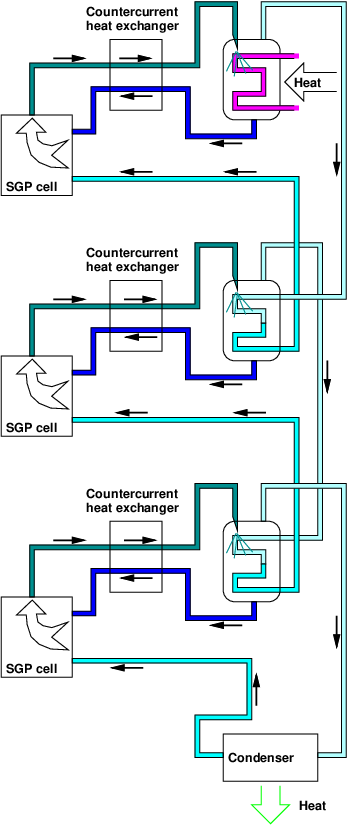
In the present section we describe the application of the concept of the multiple effects to the HTCC. A three-effect version of the HTCC is shown in Fig. 4. Each of the effects is similar to the above-described practical HTCC.
As already stated, that the main part of the heat absorbed by one of the effects is represented by the evaporation heat of the solution at the temperature , whereas the main release of heat at the temperature corresponds to the condensation heat of the solvent vapor. We couple a first stage (effect) to a second one, similar to the first one but working at a lower pressure, such that at this lower pressure the boiling temperature of the solution is equal to . Then the second stage will produce additional electrical energy by using the heat released by the condensation of the solvent vapor that goes out of the first one. Generalizing this idea, we can realize similar devices, all working with solutions of the same concentration , but at pressures such that, denoting by and respectively the boiling temperatures of the solution and of pure solvent at pressure , one has , and so on. The first device absorbs the heat at the temperature , and delivers the heat to the second device at the temperature . Heat exchanges of the same type occur between all of the subsequent devices of the chain, until the last one releases the heat to the external environment at the temperature , which may be equal to room temperature if is sufficiently low.
By using the same approximations used above, one can assume that the total system including all the devices mainly absorbs from the external source only the heat at the temperature , and releases to the environment only the heat at the temperature . We know that each effect can work close to reversibility, and thus the overall efficiency of the whole multiple-effect HTCC is given by
| (2) |
Thus we see that the multiple-effect scheme is useful when we want to exploit two heat reservoirs with a temperature difference that is larger than the boiling point elevation of the used solution.
On the other hand, in each effect the temperature difference mirrors the boiling point elevation at the working pressure . From this point of view, the use of solutions with a high boiling point elevation allows us to reduce the total number of effects needed to fully exploit a given temperature difference .
V The potential of the concentration cell
The result that the efficiency increases with the boiling point elevation comes as a surprise because the presence of a high boiling point elevation is usually connected with a lower production of distilled products. This is due to the peculiarity of the application we consider. Indeed, a higher boiling point elevation results in a higher free energy content per unit mass of produced solution, and thus to an increase of efficiency, associated to a decrease of the total flow of liquids. In the present section we discuss the relation between the thermal properties (i.e. the boiling points and the vapor pressures of the solutions) and the potential of the electrochemical cell, or, better, the chemical potential of the solute.
With reference to the single-effect ideal cycle described above, let us assume that the solution contains moles of solvent and moles of solute, contains moles of solvent, and threfore contains moles of solvent and moles of solute. The Gibbs free energies of the solutions , and at temperature are , and respectively. The electrical work produced by the SGP cell equals the total available Gibbs free energy:
| (3) |
If , the above relation can be expressed in terms of the chemical potential of the solvent as
| (4) |
So, expressing through the definition of efficiency, where is the amount of heat absorbed from an external source, one gets
| (5) |
Since in our case is roughly the heat needed for evaporating moles of the solvent, we can write , where is the latent heat of evaporation of the solvent. Finally, substituting the value of that was previously evaluated, one obtains
| (6) |
Thus we see that the molecules of the solvent feel a stronger chemical potential gradient between the concentrated solution and the pure solvent when the boiling point elevation is higher. It is worth noting that the difference of the chemical potential of the solvent between the solutions is proportional to the osmotic pressure, that is exploited in the SGP devices based on osmosis.
Now, using the formula above, the boiling point elevation can be related to the output voltage of an electrochemical SGP cell. Indeed, we can evaluate the voltage by means of the Nernst equation:
| (7) |
where is the chemical potential of the solute, is the number of electrons exchanged during the redox reaction, and and are the concentrations of the solutions in the SGP cell. In turn, can be evaluated from , by means of the relation
| (8) |
The derivation of this equation can be found in SI[38], Appendix B, together with a more rigorous procedure for the calculation of the chemical potential from the boiling point elevation. The concepts introduced in this section are also developed in SI[38], Appendix C, to obtain an alternative derivation of the efficiency for the ideal cycle.
| a |
 |
| b |
 |
To give examples of application of this procedure, we show in Fig. 5a the curves of the boiling temperatures at atmospheric pressure of aqueous solutions of NaOH and NaCl, and in Fig. 5b the resulting curves of the chemical potential of the solute at the temperature C. Both curves have been arbitrarily set to 0 at the concentration , which corresponds to 5% in weight for NaOH. Note in fact that Eq. 8 allows us to evaluate the chemical potential only up to an additional constant term, which is however irrelevant for the calculation of the potential of the cell. One can notice how the higher boiling point elevation of NaOH entails a steeper increase, with respect to NaCl, of the chemical potential as a function of the concentration. By applying Eq. 7 we obtain that a concentration cell, having in a compartment a solution of NaOH at 5% in weight, and in the other one a solution of NaOH at 50% in weight (which corresponds to a molar fraction of 0.31 and a boiling point elevation at atmospheric pressure of C), provides in the ideal case a potential of 0.31 V at C.
Acknowledgements
We thank Alessandro Atti, Pino Gherardi and Paolo Turroni for the collaboration in the development of the concept of the closed-cycle heat-to-current converter. We thank Luigi Galgani and Maarten Biesheuvel for useful discussions and suggestions on the manuscript. The research leading to these results received funding from the European Union Seventh Framework Programme (FP7/2007-2013) under agreement no. 256868, CAPMIX project.
References
- [1] R. H. Cole and J. S. Coles, Physical principles of chemistry (W. H. Freeman and Company, San Francisco, 1964).
- [2] R. E. Pattle, Nature 174, 660 (1954).
- [3] R. W. Norman, Science 186, 350 (1974).
- [4] B. E. Logan and M. Elimelech, Nature 488, 313 (2012).
- [5] S. Loeb, Desalination 120, 247 (1998).
- [6] M. Turek, B. Bandura, and P. Dydo, Desalination 221, 462 (2008).
- [7] A. Cipollina, A. Misseri, G. D’Alí Staiti, A. Galia, G. Micale, and O. Scialdone, Desalination and Water Treatment 49, 390 (2012).
- [8] O. Levenspiel and N. de Vevers, Science 183, 157 (1974).
- [9] S. Loeb, Science 189, 654 (1975).
- [10] T. S. Chung, X. Li, R. C. Ong, Q. G. H. Wang, and G. Han, Curr. Opin. Chem. Eng. 1, 246 (2012).
- [11] J. N. Weinstein and F. B. Leitz, Science 191, 557 (1976).
- [12] J. W. Post, H. V. M. Hamelers, and C. J. N. Buisman, Env. Sci. Techn. 42, 5785 (2008).
- [13] J. W. Post, J. Veerman, H. V. M. Hamelers, G. J. W. Euverink, S. J. Metz, K. Nymeijer, and C. J. N. Buisman, J. Membrane Sci. 288, 218 (2007).
- [14] B. H. Clampitt and F. E. Kiviat, Science 194, 719 (1976).
- [15] D. Brogioli, Phys. Rev. Lett. 103, 058501 (2009).
- [16] B. B. Sales, M. Saakes, J. W. Post, C. J. Buisman, P. M. Biesheuvel, and H. V. Hamelers, Env. Sci. Techn. 44, 5661 (2010).
- [17] D. Brogioli, R. Zhao, and P. M. Biesheuvel, Energ. Environ. Sci. 4, 772 (2011).
- [18] O. Burheim, B. Sales, O. Schaezle, F. Liu, and H. V. M. Hamelers, “Auto generative capacitive mixing of sea and river water by the use of membranes,” ASME 2011 International Mechanical Engineering Congress and Exposition (IMECE2011) (Denver, Colorado, USA) p. 483–492, paper no. IMECE2011-63459 (2011).
- [19] M. F. M. Bijmans, O. S. Burheim, M. Bryjak, A. Delgado, P. Hack, F. Mantegazza, S. Tennisson, and H. V. M. Hamelers, Energy Procedia 20, 108 (2012).
- [20] R. A. Rica, R. Ziano, D. Salerno, F. Mantegazza, R. van Roij, and D. Brogioli, Entropy 15, 1388 (2013).
- [21] D. Brogioli, R. Ziano, R. A. Rica, D. Salerno, and F. M. azza, J. Coll. Interf. Sci. 407, 457 (2013).
- [22] F. La Mantia, M. Pasta, H. D. Deshazer, B. E. Logan, and Y. Cui, Nano Lett. 11, 1810 (2011).
- [23] Z. Jia, B. Wang, S. Song, and Y. Fan, RSC Adv. 3, 26205 (2013).
- [24] R. L. McGinnis, J. R. McCutcheon, and M. Elimelech, J. Membr. Sci. 305, 13 (2007).
- [25] I. Tlili, Y. Timoumi, and S. Ben Nasrallah, Renew. Energ. 33, 1911 (2008).
- [26] G. J. Snyder and E. S. Toberer, Nat. Mater. 7, 105 (2008).
- [27] A. Weidenkaff, R. Robert, A. M. Aguirre, L. Bocher, T. Lippert, and S. Canulescu, Renew. Energ. 33, 342 (2008).
- [28] G. Fraisse, J. Ramousse, D. Sgorlon, and C. Goupil, Energ. Convers. Manag. 65, 351 (2013).
- [29] N. D. Kaushika and K. S. Reddy, Energ. Convers. Manag. 41, 713 (2000).
- [30] J. Muschaweck, W. Spirkl, A. Timinger, N. Benz, M. Dorfler, M. Gut, and E. Kose, Solar energy 68, 151 (2000).
- [31] W. Spirkl, H. Ries, J. Muschaweck, and R. Winston, Solar energy 62, 113 (1998).
- [32] S. A. Omer and D. G. Infield, Energ. Convers. Manag. 41, 737 (2000).
- [33] A. Rosato and S. Sibilio, Energ. Convers. Manag. 70, 149 (2013).
- [34] T. H. Pan, D. L. Xu, A. M. Li, S. S. Shieh, and S. S. Jang, Energ. Convers. Manag. 68, 169 (2013).
- [35] E. Hala, J. P. V. Fried, and O. Vilim, Vapour–liquid equilibrium (Pergamon Press, 1967).
- [36] K. S. Kim, W. Ryoo, M. S. Chun, and G. Y. Chung, Desalination 318, 79 (2013).
- [37] M. W. Zemansky, Heat and thermodynamics (Mc Graw–Hill, New York, 1957).
- [38] See supplementary material at URL for the rigorous proofs of the propositions in the paper.
- [39] A. Mclaren White, Ind. Eng. Chem. 22, 230 (1930).