FTUV/13-0913 IFIC/13-63 LA-UR-13-27104 Lepton flavor violation in the Higgs sector and the role of hadronic $\tau$-lepton decays

Flavor violating couplings of the Higgs boson to leptons arise in many extensions of the SM. If the new physics originates at a scale $\Lambda$ well above the EW scale, then an effective theory treatment is justifiable. Details of the ultraviolet completion of the SM can then be encoded in effective operators containing only the SM degrees of freedom and which can give rise to LFV effects [24, 25]. It is however possible that the new physics (NP) enters at a scale not much higher than the electroweak scale, so that these new degrees of freedom cannot be integrated out. One possibility is to consider an extended Higgs sector with several scalar fields below the TeV scale and non-diagonal Yukawa couplings in flavor space. Indeed, it is the case that a simple extension of the SM scalar sector by an additional Higgs doublet, a two-Higgs-doublet model (2HDM), gives rise to flavor-changing neutral currents (FCNCs) at tree-level in the quark and lepton sectors. Usually a symmetry principle is assumed that forbids such effects [26, 27] and allows to evade the stringent bounds coming from the Kaon and $B$-meson precision experiments. While such an approach is well justified or needed for the quark sector, one can be less restrictive in the lepton sector, while being consistent with flavor constraints.

The strongest bound on possible LFV Higgs couplings to $\tau-\ell$ ($\ell=e,\mu$) are currently obtained from $\tau\rightarrow\ell\gamma$ decays. It was first noticed in Ref. [7] that present bounds still allow for very large LFV Higgs decay rates $\mathrm{BR}(h\rightarrow\tau\ell)\lesssim 10\%$. It was later shown in Refs. [18, 19] that the LHC prospects in constraining such LFV Higgs couplings are very promising, even with present accumulated data. Constraining LFV couplings of the $125$ GeV Higgs directly at the LHC, or finding additional low-energy handles, becomes even more relevant when one considers the nature of the bound that can be extracted from $\tau\rightarrow\ell\gamma$ decays. The effective dipole operator $(\bar{\ell}\sigma^{\mu\nu}P_{L,R}\tau)F_{\mu\nu}$ giving rise to $\tau\rightarrow\ell\gamma$ decays appears at the loop-level and is very sensitive to details of the high energy dynamics. Due to the strong chirality suppression of the one-loop diagrams, the dominant contribution to the $\tau\rightarrow\ell\gamma$ decay amplitude arises from two-loop diagrams of the Barr-Zee type [28]. Additional scalars or heavy degrees of freedom belonging to the UV completion of the theory can cause sizable interfering contributions, making it impossible to extract a model independent bound on the scalar LFV couplings. This issue is circumvented at the LHC by searching directly for LFV Higgs decays, the Higgs being produced via its coupling to $VV=W^{+}W^{-},ZZ$ in vector-boson fusion and in associated Higgs production with a vector boson [18], or, relying on its loop-induced coupling to gluons in the gluon fusion mode [19].

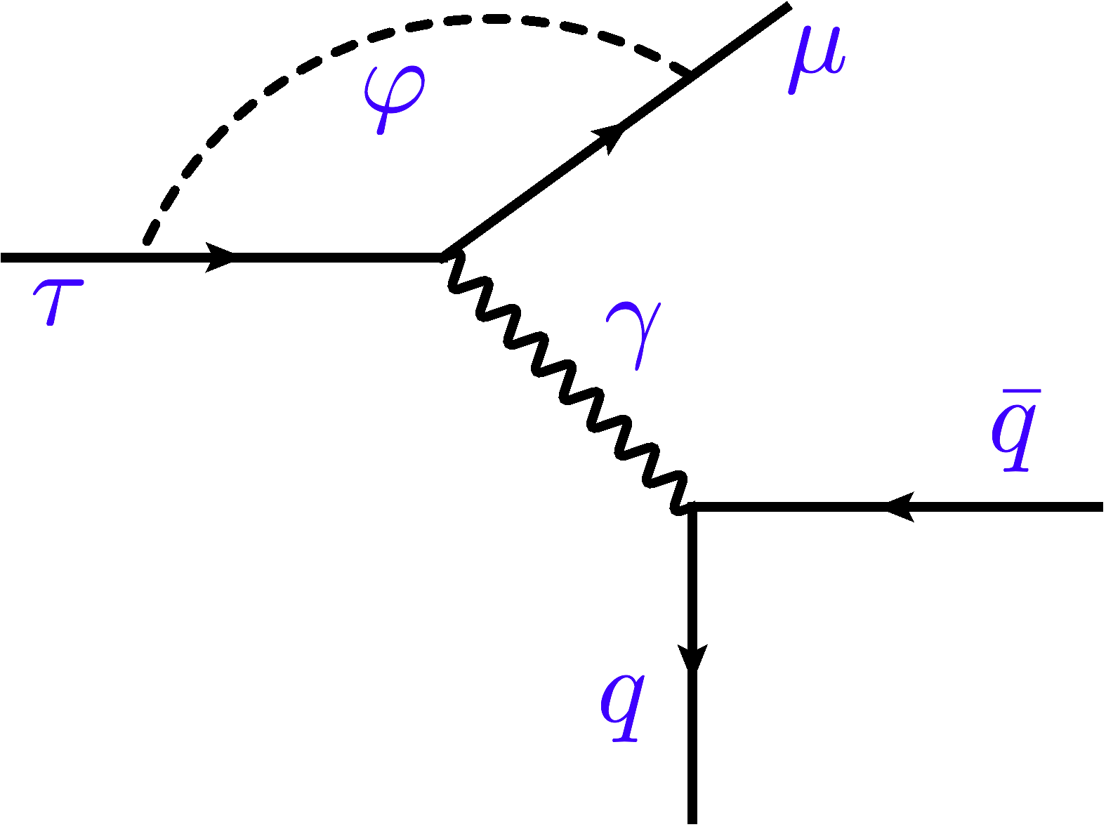
At low energy, semileptonic $\tau$ decays like $\tau\rightarrow\ell\pi\pi$ ($\pi\pi=\pi^{+}\pi^{-},\pi^{0}\pi^{0}$) offer a unique opportunity to extract a bound on the LFV Higgs couplings which is much less sensitive to details of the high energy dynamics, thus establishing a model-independent connection with the search for LFV Higgs decays at the LHC. The same effective coupling of the Higgs to gluons that would give rise to $pp(gg)\rightarrow h\rightarrow\tau\ell$, also enters in the $\tau\rightarrow\ell\pi\pi$ mode though at a much lower energy scale where non-perturbative QCD effects play a major role, see Fig. 1. Similarly, the semileptonic decays $\tau\rightarrow\ell P$ (where $P$ is a pseudoscalar meson) establish a connection with the search for LFV decays of a CP-odd Higgs at the LHC.

Calculations of $\tau\rightarrow\ell\pi\pi$ mediated by a Higgs boson with LFV couplings in the literature have mostly considered the scalar-current associated with the Higgs coupling to light quarks, thus neglecting the effective coupling of the Higgs to gluons due to intermediate heavy quarks (with the exception of Ref. [29], in which a more general EFT analysis including gluon operators is presented). Moreover, a description of the scalar-current hadronic matrix elements based on leading order predictions of Chiral-Perturbation Theory (ChPT) has been used in these works [9, 12, 14, 29]. Such treatment of the hadronic matrix elements is not adequate to deal with $\tau$ decays, for which the $\pi\pi$ invariant mass can be as large as $m_{\tau}-m_{\ell}$. It was pointed out recently in Ref. [30], within the context of R-parity violating supersymmetry, that by using a more appropriate description of the hadronic matrix elements of the scalar and vector currents, the bounds obtained on the R-parity-violating couplings improve considerably.

In this work we provide for the first time a complete description of the $\tau\rightarrow\ell\pi\pi$ mode in the presence of a Higgs boson with LFV couplings. A detailed discussion of the hadronic matrix elements involved is given. When relevant we also compare the form factors we obtain with those of previous work. With these tools in hand, we extract from $\tau\to\ell\pi\pi$ robust model-independent bounds on LFV couplings of the Higgs. The LFV decays $\tau\rightarrow\ell P$ and the relevant hadronic matrix elements in this case are also discussed, leading to bounds on LFV couplings of a CP-odd neutral scalar.

In the context of an extended Higgs sector, we also point out the importance of performing searches for additional Higgs bosons in the LFV decay modes $\tau-\mu$ and $\tau-e$ at the LHC. Present data constrain the $h(125)$ coupling to vector bosons to be very close to the SM value $g_{hVV}\simeq g_{hVV}^{\mathrm{SM}}$ [1, 2, 3]. In general two-Higgs-doublet models, any possible LFV coupling of the $125$ GeV Higgs boson at the end turns out to be suppressed by an accompanying small or vanishing mixing factor $\left(1-(g_{hVV}/g_{hVV}^{\mathrm{SM}})^{2}\right)^{1/2}$. Additional Higgs bosons which would play a minor role in the restoration of perturbative unitarity on the other hand, do not receive this suppression of their LFV couplings. The search for LFV decays associated to the scalar sector should therefore not be restricted to the $125$ GeV boson.

Our paper is organized as follows: In Sect. 2 we describe our framework. In Sect. 3 we provide a detailed discussion of the hadronic form factors relevant for the description of $\tau\rightarrow\mu\pi\pi$ decays. In Sect. 4 we describe the framework used in this work to motivate the discussion of possible LFV effects due to both CP-even and CP-odd Higgs bosons. We then consider the semileptonic LFV decay $\tau\rightarrow\mu\pi\pi$ ($\pi\pi=\pi^{+}\pi^{-},\pi^{0}\pi^{0}$) mediated by a CP-even Higgs boson, we discuss the relevance of this process in connection to other LFV transitions accessible at $B$-factories ($\tau\rightarrow\mu\gamma,3\mu,\ldots$) as well as for the LHC ($h\rightarrow\tau\mu$). The phenomenology of a CP-odd Higgs boson is also discussed along the same lines. We give our conclusions in Sect. 5.

The vector form factor $F_{V}(s)$ has been measured both directly from $e^{+}e^{-}\rightarrow\pi^{+}\pi^{-}$ [31, 32, 33, 34, 35] and via an isospin rotation from $\tau\rightarrow\pi^{-}\pi^{0}\nu_{\tau}$ [36, 37]. It has also been determined by several theoretical studies [38, 39, 40, 41, 42, 43, 44, 45, 46, 47, 48, 49, 50, 51, 52, 53, 54].

In the spirit of Refs. [52, 55, 56, 57, 58, 59, 60, 61] we determine the vector form factor phenomenologically by fitting the invariant mass distribution of $\tau\rightarrow\pi^{-}\pi^{0}\nu_{\tau}$ decays using a theoretically well-motivated parametrization. To this end, we adapt the dispersive parametrizations introduced in Refs. [52, 59] mimicking what has been done for $K\pi$ in Refs. [56, 57, 58, 62]. Note that for our purposes, the isospin-breaking corrections can be neglected. A dispersion relation with three subtractions at $s=0$ is written for ln($F_{V}(s)$). This leads to the following representation for $F_{V}(s)$ [52, 59]

$$F_{V}(s)=\mathrm{exp}\left[\lambda_{V}^{\prime}\frac{s}{M_{\pi}^{2}}+\frac{1}{2}\left(\lambda_{V}^{\prime\prime}-\lambda_{V}^{\prime 2}\right)\left(\frac{s}{M_{\pi}^{2}}\right)^{2}+\frac{s^{3}}{\pi}\int_{4M_{\pi}^{2}}^{\infty}\frac{ds^{\prime}}{s^{\prime 3}}\frac{\phi_{V}(s^{\prime})}{(s^{\prime}-s-i\epsilon)}\right]~.$$

(5)

To fix one subtraction constant, use has been made of $F_{V}(s=0)\equiv 1$ required by gauge invariance. $\lambda_{V}^{\prime}$ and $\lambda_{V}^{\prime\prime}$ are the two other subtraction constants corresponding to the slope and the curvature of the form factor. They are determined from a fit to the data. $\phi_{V}(s)$ represents the phase of the form factor. In the elastic region $\left(s\lesssim 1~\mathrm{GeV}^{2}\right)$, according to Watson theorem [63] the phase of the form factor $\phi_{V}(s)$ is equal to the P wave $I=1$ $\pi\pi$ scattering phase shift $\delta_{1}^{1}(s)$ which is known with an excellent precision from the solutions of Roy-Steiner equations [64, 65]. However for $s>1~\mathrm{GeV}^{2}$ other channels open ($4\pi,K\bar{K}$) and $\phi_{V}(s)$ is not known. Taking advantage of the precise measurements of the invariant mass distribution of $\tau\rightarrow\pi^{-}\pi^{0}\nu_{\tau}$ decays [37], the phase of the form factor can be modeled in terms of the three resonances found in this decay region and directly determined from the data.

We write $\mathrm{tan}\phi_{V}(s)=\mathrm{Im}\tilde{F}_{V}(s)/\mathrm{Re}\tilde{F}_{V}(s)$ in terms of a model for the form factor $\tilde{F}_{V}(s)$ that includes three resonances $\rho(770)$, $\rho^{\prime}(1465)$ and $\rho^{\prime\prime}(1700)$ with two mixing parameters $\alpha^{\prime}$ and $\alpha^{\prime\prime}$ measuring the relative weight between the resonances and $\phi^{\prime}$ and $\phi^{\prime\prime}$ accounting for the corresponding interferences, see Ref. [59]:

$$\tilde{F}_{V}(s)=\frac{\tilde{M}_{\rho}^{2}+\left(\alpha^{\prime}e^{i\phi^{\prime}}+\alpha^{\prime\prime}e^{i\phi^{\prime\prime}}\right)s}{\tilde{M}_{\rho}^{2}-s+\kappa_{\rho}~\mathrm{Re}\left[A_{\pi}(s)+\frac{1}{2}A_{K}(s)\right]-i\tilde{M}_{\rho}\tilde{\Gamma}_{\rho}(s)}-\frac{\alpha^{\prime}e^{i\phi^{\prime}}s}{D(\tilde{M}_{\rho^{\prime}},\tilde{\Gamma}_{\rho^{\prime}})}-\frac{\alpha^{\prime\prime}e^{i\phi^{\prime\prime}}s}{D(\tilde{M}_{\rho^{\prime\prime}},\tilde{\Gamma}_{\rho^{\prime\prime}})}~,$$

(6)

with

$$D(\tilde{M}_{R},\tilde{\Gamma}_{R})=\tilde{M}_{R}-s+\kappa_{R}\mathrm{Re}A_{\pi}(s)-i\tilde{M}_{R}\tilde{\Gamma}_{R}(s)~.$$

(7)

In this equation $\tilde{M}_{R}$ and $\tilde{\Gamma}_{R}$ are model parameters. $\tilde{\Gamma}_{R}$ and $\kappa_{R}$ are given by :

$$\tilde{\Gamma}_{R}(s)=\tilde{\Gamma}_{R}\frac{s}{\tilde{M}_{R}^{2}}\frac{\left(\sigma_{\pi}^{3}(s)+1/2~\sigma_{K}^{3}(s)\right)}{\left(\sigma_{\pi}^{3}(\tilde{M}_{R}^{2})+1/2~\sigma_{K}^{3}(\tilde{M}_{R}^{2})\right)}~,~~\kappa_{R}(s)=\frac{\tilde{\Gamma}_{R}}{\tilde{M}_{R}}\frac{s}{\pi\left(\sigma_{\pi}^{3}(\tilde{M}_{R}^{2})+1/2~\sigma_{K}^{3}(\tilde{M}_{R}^{2})\right)}~,$$

(8)

if $R\equiv\rho$ and

$$\tilde{\Gamma}_{R}(s)=\tilde{\Gamma}_{R}\frac{s}{\tilde{M}_{R}^{2}}\frac{\sigma_{\pi}^{3}(s)}{\sigma_{\pi}^{3}(\tilde{M}_{R}^{2})}~,~~\kappa_{R}(s)=\frac{\tilde{\Gamma}_{R}}{\tilde{M}_{R}}\frac{s}{\pi\sigma_{\pi}^{3}(\tilde{M}_{R}^{2})}~,$$

(9)

otherwise. This parametrization is guided by Resonance Chiral Theory (RChT) [66, 67, 68]. While RChT allows one to compute the decay width $\tilde{\Gamma}_{R}$ and $\kappa_{R}$ for the $\rho$ resonance, Eq. (8), taking into account the $\pi\pi$ and $K\bar{K}$ intermediate states [48], this is not the case anymore for $\rho^{\prime}$ and $\rho^{\prime\prime}$. Hence in Eq. (9), generic $\tilde{\Gamma}_{R}$ and $\kappa_{R}$ as expected for a vector resonance decaying only in $\pi\pi$ has been assumed¹¹ 1 The assumption that $\rho^{\prime}$ and $\rho^{\prime\prime}$ only decay in $\pi\pi$ has been made. One could improve the model by considering other decay modes as it has been done for $K\pi$ in Ref. [62]. [55]. In Eq. (6), $A_{\pi}(s)$ and $A_{K}(s)$ are the $\pi\pi$ and $K\bar{K}$ loop functions in ChPT [48, 59] and $\sigma_{\pi}$ and $\sigma_{K}$ represents the velocity of the two particles in the centre-of-mass frame:

	$\displaystyle\sigma_{\pi}(s)\!\!$	$\displaystyle\equiv$	$\displaystyle\!\!\sqrt{1-4M_{\pi}^{2}/s}~\theta\left(s-4M_{\pi}^{2}\right)~,$
	$\displaystyle\sigma_{K}(s)\!\!$	$\displaystyle\equiv$	$\displaystyle\!\!\sqrt{1-4M_{K}^{2}/s}~\theta\left(s-4M_{K}^{2}\right)~.$		(10)

Here $\theta$ denotes the Heaviside step function $\theta(x)=1$ for $x>0$, being zero otherwise. Note that the parameter $\kappa_{R}$ is defined such as $i\kappa_{R}~\mathrm{Im}A_{\pi}(s)=-i\tilde{M}_{R}\tilde{\Gamma}_{R}(s)$ with $\mathrm{Im}A_{\pi}(s)\to\mathrm{Im}[A_{\pi}(s)+1/2A_{\pi}(s)]$ for $\rho$. We emphasize here that $\tilde{M}_{R}$ and $\tilde{\Gamma}_{R}$ are model parameters and do not correspond to the physical resonance mass and width. To find them one has to find the pole of each term of Eq. (6) or equivalently the zeros of their denominator Eq. (7) on the second Riemman sheet.

The model used to determine $\phi_{V}$, Eq. (6), inspired by the Gounaris-Sakurai parametrization [39] is only valid in the $\tau$ decay region and is therefore only used in Eq. (5) for $s\leq s_{\mathrm{cut}}\sim m_{\tau}^{2}$. For the high-energy region of the dispersive integral Eq. (5) ($s>s_{\mathrm{cut}}\sim m_{\tau}^{2}$) the phase is unknown and following Refs. [58, 69, 62] we take a conservative interval between 0 and $2\pi$ centered at the asymptotic value of the phase of the form factor which is $\pi$. Indeed perturbative QCD dictates the asymptotic behavior of the form factor: it should vanish as $\mathcal{O}(1/s)$ up to logarithmic corrections [70] for large values of $s$ implying that its phase should asymptotically reach $\pi$. The use of a three-time subtracted dispersion relation reduces the impact of our ignorance of the phase at relative high energies in Eq. (5). However, in order for the form factor to have the correct asymptotic behavior two sum rules have to be satisfied:

$$\lambda_{V}^{\prime~\mathrm{sr}}=\frac{m_{\pi}^{2}}{\pi}\int_{4M_{\pi}^{2}}^{\infty}ds^{\prime}\frac{\phi_{V}(s^{\prime})}{s^{\prime 2}}~,$$

(11)

$$(\lambda_{V}^{\prime\prime}-\lambda_{V}^{\prime 2})^{\mathrm{sr}}=\frac{2m_{\pi}^{4}}{\pi}\int_{4M_{\pi}^{2}}^{\infty}ds^{\prime}\frac{\phi_{V}(s^{\prime})}{s^{\prime 3}}\equiv\alpha_{2v}^{\mathrm{sr}}~.$$

(12)

They are used to constrain the fit to the data as done for $K\pi$ in Refs. [58, 62].

Twelve parameters entering $F_{V}(s)$, Eq. (5) are therefore determined by a fit to the data:

• •

  $\lambda_{V}^{\prime}$ and $\lambda_{V}^{\prime\prime}$, the two subtraction constants

• •

  $\tilde{M}_{\rho}$ and $\Gamma_{\rho}$, $\tilde{M}_{\rho^{\prime}}$ and $\Gamma_{\rho^{\prime}}$, $\tilde{M}_{\rho^{\prime\prime}}$ and $\Gamma_{\rho^{\prime\prime}}$ the mass and decay width of $\rho(770)$, $\rho^{\prime}(1465)$ and $\rho^{\prime\prime}(1700)$ respectively used to model the phase

• •

  $\alpha^{\prime}$, $\alpha^{\prime\prime}$ and their phases $\phi^{\prime}$, $\phi^{\prime\prime}$ the mixing parameters between the resonances

The following quantity is minimized :

$$\chi^{2}=\sum_{i=1}^{62}\left(\frac{\left(|F_{V}(s)|^{2}\right)_{i}^{\mathrm{theo}}-\left(|F_{V}(s)|^{2}\right)_{i}^{\mathrm{exp}}}{\sigma_{\left(|F_{V}(s)|^{2}\right)_{i}^{\mathrm{exp}}}}\right)^{2}+\left(\frac{\lambda_{V}^{\prime}-\lambda_{V}^{\prime~\mathrm{sr}}}{\sigma_{\lambda_{V}^{\prime~\mathrm{sr}}}}\right)^{2}+\left(\frac{\alpha_{2v}-\alpha_{2v}^{\mathrm{sr}}}{\sigma_{\alpha_{2v}^{\mathrm{sr}}}}\right)^{2}~,$$

(13)

with $\left(|F_{V}(s)|^{2}\right)^{\mathrm{exp}}$ and its uncertainty $\sigma_{\left(|F_{V}(s)|^{2}\right)\mathrm{exp}}$, the modulus squared of the vector form factor experimentally extracted from the measurement of the $\tau^{-}\to\pi^{-}\pi^{0}\nu_{\tau}$ invariant decay distribution [37] and $F_{V}(s)^{\mathrm{theo}}$ the form factor parametrized in Eq. (5). In addition to the first term also minimized in previous analyses [37, 59], we impose the constraints given by the two sum rules Eqs. (11) and (12)²² 2 $\sigma_{\lambda_{V}^{\prime~\mathrm{sr}}}$ and $\sigma_{\alpha_{2v}^{\mathrm{sr}}}$ are given by the $2\pi$ band taken for the high energy phase. to guarantee the correct asymptotic behaviour of the form factor. This allows us to have a description for the form factor, Eq. (5) that not only fulfills the properties of analyticity and unitarity but is also in agreement with perturbative QCD. This is not the case for the dispersive representations of Refs. [52, 59] and for the parametrization used by Belle collaboration to fit their data [37].

The result of the fit is given in Tab. 1 and shown in Fig. 3 together with the Belle data. As can been seen from the figure and the $\chi^{2}$, the agreement with data is excellent. Note that we have presented here a description for the form factor that represents the state-of-the-art, in that it relies on the fewest model assumptions and is valid on a large energy range. For the purposes of bounding LFV Higgs couplings, a parametrization a la Gounaris-Sakurai that describes well the data as the one used in Ref. [37] could have been sufficient.

The scalar form factors and $\theta_{\pi}(s)$ cannot be determined so directly and unambiguously from the data. However, they can be reconstructed from dispersive theory with a matching at low-energy to ChPT as pioneered in Ref. [71]. As we have seen, elastic unitarity only holds at low-energy for $s\ll 1$ GeV² and in the scalar case it is very well known that the elastic approximation breaks down for the $\pi\pi$ $S$-wave already at the $K\bar{K}$ threshold due to the strong inelastic coupling of two $S$-wave pions to $K\bar{K}$ in the region of $f_{0}(980)$. In order to describe the scalar form factors in the kinematical region needed for $\tau\to\ell\pi\pi$, one has to solve a two-channel Mushkhelishvili-Omnès problem following Refs. [71, 72] including $\pi\pi$ and $K\bar{K}$ scattering. As $s$ increases, a new two-body channel opens: $\eta\eta$. At some point, the $4\pi$-channel will also become important. As discussed in Refs. [73, 72], below $\sqrt{s}\sim 1.4$ GeV the inelasticity is found to be saturated to a good approximation by a single channel $K\bar{K}$.

Two-Higgs-doublet models (2HDM) provide a specific gauge-invariant framework where lepton flavor violating effects encoded in Eq. (1) can occur, due to both CP-even and CP-odd Higgs bosons at tree-level. In the Higgs basis, where only one scalar doublet acquires a vev, one can write [26]

$\displaystyle\Phi_{1}=\begin{pmatrix}G^{+}\\ \frac{1}{\sqrt{2}}(v+S_{1}+iG^{0})\end{pmatrix}\,,\qquad\Phi_{2}=\begin{pmatrix}H^{+}\\ \frac{1}{\sqrt{2}}(S_{2}+iS_{3})\end{pmatrix}\,.$

(28)

The fields $S_{1,2}$ are CP-even while $S_{3}$ is a CP-odd field. The most general Yukawa Lagrangian of the 2HDM is given by

	$\displaystyle\mathcal{L}_{Y}\;=$	$\displaystyle\;-\frac{\sqrt{2}}{v}\Bigl\{\bar{L}_{L}^{\prime}\,\left(M_{\ell}^{\prime}\,\Phi_{1}+\Pi_{\ell}^{\prime}\,\Phi_{2}\right)\,\ell_{R}^{\prime}$
		$\displaystyle+\bar{Q}_{L}^{\prime}\,\left(M_{d}^{\prime}\,\Phi_{1}+\Pi_{d}^{\prime}\,\Phi_{2}\right)\,d_{R}^{\prime}+\bar{Q}_{L}^{\prime}\,\left(M_{u}^{\prime}\,\tilde{\Phi}_{1}+\Pi_{u}^{\prime}\,\tilde{\Phi}_{2}\right)\,u_{R}^{\prime}\Bigr\}+\mathrm{h.c.}\,,$		(29)

where $\bar{L}_{L}^{\prime}=\left(\bar{\nu}_{L}^{\prime},\bar{\ell}_{L}^{\prime}\right)$ is the left-handed lepton doublet, $Q_{L}^{\prime}=(u_{L}^{\prime},d_{L}^{\prime})$ is the left-handed quark doublet and $\ell_{R}^{\prime},u_{R}^{\prime},d_{R}^{\prime}$ are right-handed SU(2) singlets in flavor space. The primes over the fields and couplings denote that we are still in an arbitrary weak basis, the usual notation $\tilde{\Phi}=i\tau_{2}\Phi^{*}$ is used. The matrices $M_{f=u,d,\ell}^{\prime}$ represent the non-diagonal fermion mass matrices while $\Pi_{f=u,d,\ell}^{\prime}$ are arbitrary complex matrices in flavor space parametrizing the Yukawa couplings of the second Higgs doublet $\Phi_{2}$.

After EWSB the neutral mass eigenstates $\varphi_{k}=\{h,H,A\}$ are obtained via an orthogonal transformation, $\varphi_{k}=\mathcal{R}_{km}\,S_{m}$, that diagonalizes the mass matrix of the scalar fields ($M_{h}\leq M_{H}$ in our conventions). The Higgs couplings to vector bosons $(VV=W^{+}W^{-},ZZ)$ are given by $g_{\varphi_{k}VV}=\mathcal{R}_{k1}\,g^{\mathrm{SM}}_{hVV}$, where $g^{\mathrm{SM}}_{hVV}$ represents the SM gauge coupling, while the interactions of the physical scalars $\{h,H,A,H^{\pm}\}$ with fermions are described by

	$\displaystyle\mathcal{L}_{Y}$	$\displaystyle=$	$\displaystyle-\,\sum_{\varphi_{k},f=u,d,\ell}\,\varphi_{k}\,\bar{f}\,Y_{f}^{\varphi_{k}}\,P_{R}\,f$		(30)
			$\displaystyle-\frac{\sqrt{2}}{v}\,H^{+}\,\left\{\bar{u}\left[V\,\Pi_{d}\,P_{R}-\Pi_{u}^{{\dagger}}\,V\,P_{L}\right]d\,+\bar{\nu}\,\Pi_{\ell}\,P_{R}\,\ell\,\right\}+\;\mathrm{h.c.}\,.$

Here $V$ represents the CKM matrix, $P_{L,R}=(1\mp\gamma_{5})/2$ are the usual chirality projectors and

	$\displaystyle v\,Y_{d,\ell}^{\varphi_{k}}$	$\displaystyle=M_{d,\ell}\,\mathcal{R}_{k1}+\Pi_{d,\ell}\,\left(\mathcal{R}_{k2}+i\,\mathcal{R}_{k3}\right)\,,$
	$\displaystyle v\,Y_{u}^{\varphi_{k}}$	$\displaystyle=M_{u}\,\mathcal{R}_{k1}+\Pi_{u}\,\left(\mathcal{R}_{k2}-i\,\mathcal{R}_{k3}\right)\,,$		(31)

where $M_{f=u,d,l}$ are the diagonal fermion mass matrices and $\Pi_{f=u,d,l}$ remain arbitrary complex matrices in the most general case, giving rise to tree-level FCNCs. In the Type III 2HDM [83] for example, one assumes a Yukawa structure of the form $(\Pi_{f})_{ij}\;=\;\lambda_{ij}\,\sqrt{m_{i}m_{j}}$, where the dimensionless parameters $\lambda_{ij}$ are in principle of $\mathcal{O}(1)$. Note that due to the orthogonality of the mixing matrix $\mathcal{R}$, the scalar couplings satisfy the following sum rule

$$\sum_{k}(Y_{f}^{\varphi_{k}})_{ij}\,\mathcal{R}_{k1}\;=\;0\,\qquad\text{for}~i\neq j\,.$$

(32)

In the CP-conserving limit of the 2HDM, the matrices $\Pi_{f}$ are real and the physical fields $\varphi_{k}$ have definite CP-quantum numbers. The field $A=S_{3}$ is CP-odd while the CP-even fields $h,H$ are a mixture of $S_{1,2}$,

$$\left(\begin{array}[]{c}h\\ H\\ A\end{array}\right)\;=\;\left[\begin{array}[]{ccc}\cos{\tilde{\alpha}}&\sin{\tilde{\alpha}}&0\\ -\sin{\tilde{\alpha}}&\cos{\tilde{\alpha}}&0\\ 0&0&1\\ \end{array}\right]\;\left(\begin{array}[]{c}S_{1}\\ S_{2}\\ S_{3}\end{array}\right)\,,$$

(33)

where $\tilde{\alpha}$ is a real rotation angle which can be expressed in terms of the Higgs potential parameters⁴⁴ 4 See Ref. [84] for a discussion of the 2HDM scalar potential in the CP-conserving limit as well as in the CP-violating case.. Comparing with the generic Lagrangian presented in Eq. (1) we derive the following matching for the CP-conserving limit,

	$\displaystyle Y_{ij}^{h}\;$	$\displaystyle=\;\frac{(M_{f})_{ij}}{v}\cos\tilde{\alpha}+\frac{(\Pi_{f})_{ij}}{v}\,\sin\tilde{\alpha}\,,$
	$\displaystyle Y_{ij}^{H}\;$	$\displaystyle=\;-\frac{(M_{f})_{ij}}{v}\sin\tilde{\alpha}+\frac{(\Pi_{f})_{ij}}{v}\,\,\cos\tilde{\alpha}\,,$
	$\displaystyle Y_{ij}^{A}\;$	$\displaystyle=\;\pm i\,\frac{(\Pi_{f})_{ij}}{v}\,\,.$		(34)

The plus sign in the expression for $Y_{ij}^{A}$ is for $f=d,\ell$ while the minus sign is for $f=u$. In this limit $g_{hVV}=\cos\tilde{\alpha}\,g^{\mathrm{SM}}_{hVV}$, $g_{HVV}=-\sin\tilde{\alpha}\,g^{\mathrm{SM}}_{hVV}$ and $g_{AVV}=0$. We can see that certain relations between the LFV scalar couplings arise in this case. The fermionic couplings of the lightest CP-even Higgs are flavor conserving in the limit $g_{hVV}=g^{\mathrm{SM}}_{hVV}$, and, in general these are suppressed by the factor $\sin\tilde{\alpha}$. Flavor-changing couplings of the CP-odd Higgs on the other hand do not receive such suppression. Considering the 2HDM to be a low-energy effective theory, the effect of heavy degrees of freedom contained in a UV completion will in general introduce corrections to Eq. (34), spoiling these specific relations. The effective Lagrangian of dimension-six for example contains the following terms that modify the Yukawa structure of the 2HDM,

$$\mathcal{L}_{d=6}\supset\sum_{p,r,s}\frac{1}{\Lambda^{2}}\left(C^{prs}_{\ell}\,\Phi_{p}^{{\dagger}}\Phi_{r}\,(\bar{L}_{L}\,\ell_{R}\,\Phi_{s})\,+\mathrm{h.c.}\right)+\cdots\,,$$

(35)

where $\Lambda$ represents the scale of new physics (beyond the 2HDM) and $C^{prs}_{\ell}$ are arbitrary coefficients with the role of dimensionless low-energy constants that encode the high-energy dynamics. Corrections of the type (35) are in general very small since these are suppressed by inverse powers of the high energy scale $\Lambda$. For the LFV couplings however these corrections can become relevant since it is possible that these couplings vanish or are very small in the low-energy theory.

References

- [1] CMS-Collaboration, 2013, CMS-PAS-HIG-13-005.
- [2] ATLAS-Collaboration, (2013), ATLAS-CONF-2013-034, ATLAS-COM-CONF-2013-035.
- [3] K. Cheung, J. S. Lee, and P.-Y. Tseng, JHEP 1305, 134 (2013), 1302.3794.
- [4] J. Ellis and T. You, JHEP 1306, 103 (2013), 1303.3879.
- [5] A. Falkowski, F. Riva, and A. Urbano, (2013), 1303.1812.
- [6] P. P. Giardino, K. Kannike, I. Masina, M. Raidal, and A. Strumia, (2013), 1303.3570.
- [7] G. Blankenburg, J. Ellis, and G. Isidori, Phys.Lett. B712, 386 (2012), 1202.5704.
- [8] J. L. Diaz-Cruz and J. Toscano, Phys.Rev. D62, 116005 (2000), hep-ph/9910233.
- [9] D. Black, T. Han, H.-J. He, and M. Sher, Phys.Rev. D66, 053002 (2002), hep-ph/0206056.
- [10] K. Babu and C. Kolda, Phys.Rev.Lett. 89, 241802 (2002), hep-ph/0206310.
- [11] A. Brignole and A. Rossi, Nucl.Phys. B701, 3 (2004), hep-ph/0404211.
- [12] S. Kanemura, T. Ota, and K. Tsumura, Phys.Rev. D73, 016006 (2006), hep-ph/0505191.
- [13] P. Paradisi, JHEP 0602, 050 (2006), hep-ph/0508054.
- [14] E. Arganda, M. Herrero, and J. Portoles, JHEP 0806, 079 (2008), 0803.2039.
- [15] M. Herrero, J. Portoles, and A. Rodriguez-Sanchez, Phys.Rev. D80, 015023 (2009), 0903.5151.
- [16] S. Davidson and G. J. Grenier, Phys.Rev. D81, 095016 (2010), 1001.0434.
- [17] A. Goudelis, O. Lebedev, and J.-h. Park, Phys.Lett. B707, 369 (2012), 1111.1715.
- [18] R. Harnik, J. Kopp, and J. Zupan, JHEP 1303, 026 (2013), 1209.1397.
- [19] S. Davidson and P. Verdier, Phys.Rev. D86, 111701 (2012), 1211.1248.
- [20] A. Crivellin, A. Kokulu, and C. Greub, Phys.Rev. D87, 094031 (2013), 1303.5877.
- [21] A. Dery, A. Efrati, Y. Hochberg, and Y. Nir, JHEP 1305, 039 (2013), 1302.3229.
- [22] A. Arhrib, Y. Cheng, and O. C. Kong, Phys.Rev. D87, 015025 (2013), 1210.8241.
- [23] M. Arana-Catania, E. Arganda, and M. Herrero, (2013), 1304.3371.
- [24] W. Buchmuller and D. Wyler, Nucl.Phys. B268, 621 (1986).
- [25] B. Grzadkowski, M. Iskrzynski, M. Misiak, and J. Rosiek, JHEP 1010, 085 (2010), 1008.4884.
- [26] J. F. Gunion, H. E. Haber, G. L. Kane, and S. Dawson, Front.Phys. 80, 1 (2000).
- [27] G. Branco et al., Phys.Rept. 516, 1 (2012), 1106.0034.
- [28] D. Chang, W. Hou, and W.-Y. Keung, Phys.Rev. D48, 217 (1993), hep-ph/9302267.
- [29] A. A. Petrov and D. V. Zhuridov, (2013), 1308.6561.
- [30] J. Daub, H. Dreiner, C. Hanhart, B. Kubis, and U. Meissner, JHEP 1301, 179 (2013), 1212.4408.
- [31] NA7 Collaboration, S. Amendolia et al., Nucl.Phys. B277, 168 (1986).
- [32] KLOE Collaboration, A. Aloisio et al., Phys.Lett. B606, 12 (2005), hep-ex/0407048.
- [33] CMD-2 Collaboration, R. Akhmetshin et al., Phys.Lett. B648, 28 (2007), hep-ex/0610021.
- [34] BaBar Collaboration, B. Aubert et al., Phys.Rev.Lett. 103, 231801 (2009), 0908.3589.
- [35] KLOE Collaboration, F. Ambrosino et al., Phys.Lett. B700, 102 (2011), 1006.5313.
- [36] CLEO Collaboration, S. Anderson et al., Phys.Rev. D61, 112002 (2000), hep-ex/9910046.
- [37] Belle Collaboration, M. Fujikawa et al., Phys.Rev. D78, 072006 (2008), 0805.3773.
- [38] ALEPH Collaboration, R. Barate et al., Z.Phys. C76, 15 (1997).
- [39] G. Gounaris and J. Sakurai, Phys.Rev.Lett. 21, 244 (1968).
- [40] J. Gasser and H. Leutwyler, Annals Phys. 158, 142 (1984).
- [41] T. N. Truong, Phys.Rev.Lett. 61, 2526 (1988).
- [42] J. H. Kuhn and A. Santamaria, Z.Phys. C48, 445 (1990).
- [43] J. Gasser and U. G. Meissner, Nucl.Phys. B357, 90 (1991).
- [44] G. Colangelo, M. Finkemeier, and R. Urech, Phys.Rev. D54, 4403 (1996), hep-ph/9604279.
- [45] L. v. Dung and T. N. Truong, (1996), hep-ph/9607378.
- [46] T. Hannah, Phys.Rev. D54, 4648 (1996), hep-ph/9611307.
- [47] T. Hannah, Phys.Rev. D55, 5613 (1997), hep-ph/9701389.
- [48] F. Guerrero and A. Pich, Phys.Lett. B412, 382 (1997), hep-ph/9707347.
- [49] J. Bijnens, G. Colangelo, and P. Talavera, JHEP 9805, 014 (1998), hep-ph/9805389.
- [50] J. Oller, E. Oset, and J. Palomar, Phys.Rev. D63, 114009 (2001), hep-ph/0011096.
- [51] J. De Troconiz and F. Yndurain, Phys.Rev. D65, 093001 (2002), hep-ph/0106025.
- [52] A. Pich and J. Portoles, Phys.Rev. D63, 093005 (2001), hep-ph/0101194.
- [53] B. Ananthanarayan, I. Caprini, and I. S. Imsong, Phys.Rev. D83, 096002 (2011), 1102.3299.
- [54] C. Hanhart, Phys.Lett. B715, 170 (2012), 1203.6839.
- [55] M. Jamin, A. Pich, and J. Portoles, Phys.Lett. B640, 176 (2006), hep-ph/0605096.
- [56] M. Jamin, A. Pich, and J. Portoles, Phys.Lett. B664, 78 (2008), 0803.1786.
- [57] D. Boito, R. Escribano, and M. Jamin, JHEP 1009, 031 (2010), 1007.1858.
- [58] V. Bernard, D. Boito, and E. Passemar, Nucl.Phys.Proc.Suppl. 218, 140 (2011), 1103.4855.
- [59] D. G. Dumm and P. Roig, (2013), 1301.6973.
- [60] S. Descotes-Genon, E. Kou, and B. Moussallam, (2013), 1303.2879.
- [61] R. Escribano, S. González-Solís, and P. Roig, (2013), 1307.7908.
- [62] V. Bernard, D. Boito, and E. Passemar, 2013, Work in preparation.
- [63] K. M. Watson, Phys.Rev. 88, 1163 (1952).
- [64] B. Ananthanarayan, G. Colangelo, J. Gasser, and H. Leutwyler, Phys.Rept. 353, 207 (2001), hep-ph/0005297.
- [65] I. Caprini, G. Colangelo, and H. Leutwyler, 2013, Work in preparation.
- [66] G. Ecker, J. Gasser, A. Pich, and E. de Rafael, Nucl.Phys. B321, 311 (1989).
- [67] G. Ecker, J. Gasser, H. Leutwyler, A. Pich, and E. de Rafael, Phys.Lett. B223, 425 (1989).
- [68] V. Cirigliano, G. Ecker, M. Eidemuller, A. Pich, and J. Portoles, Phys.Lett. B596, 96 (2004), hep-ph/0404004.
- [69] V. Bernard, M. Oertel, E. Passemar, and J. Stern, Phys.Rev. D80, 034034 (2009), 0903.1654.
- [70] G. P. Lepage and S. J. Brodsky, Phys.Rev. D22, 2157 (1980).
- [71] J. F. Donoghue, J. Gasser, and H. Leutwyler, Nucl.Phys. B343, 341 (1990).
- [72] B. Moussallam, Eur.Phys.J. C14, 111 (2000), hep-ph/9909292.
- [73] K. Au, D. Morgan, and M. Pennington, Phys.Rev. D35, 1633 (1987).
- [74] N. Muskhelishvili, 1953, Singular integral equations.
- [75] R. Omnes, Nuovo Cim. 8, 316 (1958).
- [76] S. Roy, Phys.Lett. B36, 353 (1971).
- [77] R. Garcia-Martin, R. Kaminski, J. Pelaez, J. Ruiz de Elvira, and F. Yndurain, Phys.Rev. D83, 074004 (2011), 1102.2183.
- [78] P. Buettiker, S. Descotes-Genon, and B. Moussallam, Eur.Phys.J. C33, 409 (2004), hep-ph/0310283.
- [79] B. Moussallam, Eur.Phys.J. C71, 1814 (2011), 1110.6074.
- [80] G. Colangelo et al., Eur.Phys.J. C71, 1695 (2011), 1011.4408.
- [81] V. Bernard, S. Descotes-Genon, and G. Toucas, JHEP 1206, 051 (2012), 1203.0508.
- [82] M. A. Shifman, A. Vainshtein, and V. I. Zakharov, Phys.Lett. B78, 443 (1978).
- [83] T. Cheng and M. Sher, Phys.Rev. D35, 3484 (1987).
- [84] A. Celis, V. Ilisie, and A. Pich, JHEP 1307, 053 (2013), 1302.4022.
- [85] Belle Collaboration, Y. Miyazaki et al., Phys.Lett. B699, 251 (2011), 1101.0755.
- [86] Belle Collaboration, Y. Miyazaki et al., Phys.Lett. B719, 346 (2013), 1206.5595.
- [87] CLEO Collaboration, G. Bonvicini et al., Phys.Rev.Lett. 79, 1221 (1997), hep-ex/9704010.
- [88] BaBar Collaboration, B. Aubert et al., Phys.Rev.Lett. 104, 021802 (2010), 0908.2381.
- [89] K. Hayasaka et al., Phys.Lett. B687, 139 (2010), 1001.3221.
- [90] W. Altmannshofer, S. Gori, and G. D. Kribs, Phys.Rev. D86, 115009 (2012), 1210.2465.
- [91] V. Barger, L. L. Everett, H. E. Logan, and G. Shaughnessy, (2013), 1308.0052.
- [92] D. Lopez-Val, T. Plehn, and M. Rauch, (2013), 1308.1979.
- [93] T. Feldmann, P. Kroll, and B. Stech, Phys.Rev. D58, 114006 (1998), hep-ph/9802409.
- [94] M. Beneke and M. Neubert, Nucl.Phys. B651, 225 (2003), hep-ph/0210085.
- [95] D. J. Gross, S. Treiman, and F. Wilczek, Phys.Rev. D19, 2188 (1979).
- [96] BaBar Collaboration, B. Aubert et al., Phys.Rev.Lett. 98, 061803 (2007), hep-ex/0610067.
- [97] ATLAS Collaboration, G. Aad et al., JHEP 1302, 095 (2013), 1211.6956.
- [98] R. V. Harlander, S. Liebler, and H. Mantler, Computer Physics Communications 184, 1605 (2013), 1212.3249.
- [99] R. V. Harlander and W. B. Kilgore, Phys.Rev.Lett. 88, 201801 (2002), hep-ph/0201206.
- [100] D. Eriksson, J. Rathsman, and O. Stal, Comput.Phys.Commun. 181, 189 (2010), 0902.0851.
- [101] K. A. Assamagan, A. Deandrea, and P.-A. Delsart, Phys.Rev. D67, 035001 (2003), hep-ph/0207302.