Finite-Temperature Phase Transition to a Quantum Spin Liquid in a Three-Dimensional Kitaev Model on a Hyperhoneycomb Lattice

The numerical results for the effective model in Eq. (3) are presented in Fig. 4. Figure 4(a) shows the internal energy per site defined by

where $\langle\cdots\rangle$ denotes the thermal average. As shown in the inset of Fig. 4(a), $T$ dependence of $E$ largely deviates from $-\tanh(T^{-1})$ that is expected for a free Ising moment in a magnetic field $J_{\rm eff}=1$; $E$ does not change so much up to $T=T_{c}\simeq 1.92$, while it rapidly increases for $T>T_{c}$. The deviation is due to the constraints on the Ising-type variables $B_{p}$, and the kink behavior around $T_{c}$ suggests a phase transition. Indeed, $E$ shows a significant system-size dependence, as shown in Fig. 4(a). Accordingly, the specific heat, calculated by

exhibits a sharp peak around $T_{c}$ which grows with increasing the system size; $C$ divided by $T$ is plotted in Fig. 4(b). The size dependence of the peak temperature of $C$, $T_{c}^{(L)}$, is presented in the inset of Fig. 4(b). The extrapolation of $T_{c}^{(L)}$ to $L\to\infty$ gives an estimate of the critical temperature as $T_{c}=1.921(1)$. The results indicate that there is a phase transition at $T=T_{c}$. The transition is not discontinuous; we see no sign of a double peak in the energy histograms (not shown).

Figure 4(c) shows the result for the entropy per site, which is calculated by the numerical integration,

$S$ appears to saturate at a much smaller value than $\ln 2$ at $T\to\infty$, as shown in the inset. The saturation value is close to $\frac{1}{2}\ln 2\sim 0.347$. This is due to the local constraint which allows $B_{p}$ to take only a half of $2^{4}$ configurations on every tetrahedron. Note that the value of the entropy corresponds to the degree of freedom in the space of the PS $\bm{\tau}_{m}$ on the diamond lattice; the number of sites on the diamond lattice in Fig. 1(b) is a half of that on the pyrochlore lattice in Fig. 1(c) as well as the original hyperhoneycomb lattice in Fig. 1(a). Interestingly, most of the entropy is released not at the transition but in the high-$T$ phase while decreasing $T$. This suggests a strong short-range correlation between the variables $B_{p}$ even well above $T_{c}$. This corresponds to the development of short-range correlations in the variables $B_{p}$ even well above $T_{c}$. Such correlations are indicated in the dynamical spin correlation function calculated in Sec. IV.3. They are also seen in terms of loops; the high-$T$ phase has a Coulombic nature due to the local constraints, as discussed in Sec. IV.4.

In this section, we calculate the magnetic susceptibility in terms of the original spins $\bm{S}_{i}$ in Eq. (1) in magnetic field applied parallel to the $z$ direction. According to the Kubo formula, the susceptibility is calculated as

In the limit of $J_{z}\gg J$, $\chi^{zz}$ can be expressed by PS operators $\bm{\tau}_{m}$ as

Here, we introduce the factor 2 to renormalize $\chi^{zz}$ by $N_{d}=N/2$ which is the site number of the diamond lattice composed of the dimers of $z$-bonds [see Fig. 1(b)].

In order to calculate the susceptibility in Eq. (9), we introduce $\tilde{\cal H}_{\rm eff}^{m}$ so as to satisfy the relation $\tau_{m}^{z}{\cal H}_{\rm eff}=\tilde{\cal H}_{\rm eff}^{m}\tau_{m}^{z}$. For a given dimer site $m$, the operator $\tau_{m}^{z}$ commutes with all $B_{p}$ that do not involve the site $m$ in the loop $p$. On the other hand, for $B_{p}$ involving the site $m$, the commutation relation between $B_{p}$ and $\tau_{m}^{z}$ depends on the location of $m$ on the loop $p$ as follows. All $B_{p}$ include two $\tau_{m}^{z}$, as shown in Fig. 2. We term such two sites $m_{1}^{p}$ and $m_{2}^{p}$. If $m$ is equal to either $m_{1}^{p}$ or $m_{2}^{p}$, $B_{p}$ commutes with $\tau_{m}^{z}$. Otherwise, $B_{p}$ anticommutes with $\tau_{m}^{z}$. The number of $B_{p}$ that anticommute with the given operator $\tau_{m}^{z}$ is eight; the eight $B_{p}$ form a loop. There are two kinds of such eight-site loops, as shown in Fig. 5. We define the set of $p$ for such $B_{p}$ as ${\cal A}_{m}$. From the definition of ${\cal A}_{m}$, $\tilde{\cal H}_{\rm eff}^{m}$ is written by

where ${\cal Q}_{m}$ is the sum of $B_{p}$ belonging to ${\cal A}_{m}$. Note that ${\cal Q}_{m}$ takes the values $-8,-6,-4,\cdots,8$. Then, the magnetic susceptibility in Eq. (9) is rewritten as

where

In Eq. (11), we used the fact that there is no spatial correlation between $\tau^{z}$, i.e., $\langle\tau_{m}^{z}\tau_{n}^{z}\rangle=\delta_{mn}$, where $\delta_{mn}$ is the Kronecker delta. This is because, in the original Kitaev model given in Eq. (1), the equal-time spin correlation $\langle S_{i}^{l}S_{j}^{l}\rangle$ is nonzero only if the sites $i$ and $j$ are on the same NN $l$-bond due to the existence of the local conserved quantity $K_{p}$. [14]

The numerical result for the magnetic susceptibility is presented in Fig. 6(a). In the high-$T$ region, the susceptibility obeys the Curie law rather than the Curie-Weiss law, i.e., Curie-Weiss temperature is exactly zero. The vanishing Curie-Weiss temperature is due to the absence of correlation between $\tau^{z}$ mentioned above. It is worthy noting that, as the effective model in Eq. (3) is justified for $T\ll J_{z}$, the Curie law behavior is considered to be seen in the temperature range $J\ll T\ll J_{z}$; in the original Kitaev model in Eq. (1), $\chi^{zz}$ should obey the Curie-Weiss law with a positive Weiss temperature proportional to $J_{z}$ for $T\gg J_{z}$. The anticipated crossover at $T\sim J_{z}$ is due to the fermion excitations which are prohibited in the effective model in Eq. (3).

While decreasing $T$, $\chi^{zz}$ deviates from the Curie law, and shows a broad hump at $T\simeq 3$. Below the hump, it rapidly decreases toward $T_{c}$ and does not strongly depend on $T$ below $T_{c}$. In the low-$T$ limit, $\chi^{zz}$ converges to a nonzero constant. Since the ground state is not degenerate in terms of $B_{p}$, the low-$T$ behavior of the susceptibility is interpreted as the Van Vleck-type paramagnetism. As explained in Appendix A, the asymptotic value for $T\to 0$ is analytically obtained to be $1/8$. Our result in Fig. 6(a) is consistent with this estimate.

As shown in Fig. 6(b), the susceptibility changes continuously in the vicinity of $T_{c}$, while showing substantial system-size dependence, similar to the internal energy and entropy shown in Figs. 4(a) and 4(c), respectively. Figure 6(c) shows $T$ derivative of the susceptibility near $T_{c}$. A sharp peak which grows with increasing the system size is observed around $T_{c}$. This implies divergent behavior of $d\chi^{zz}/dT$ at $T_{c}$.

We also analyze the behavior of $\chi^{zz}$ below $T_{c}$ by the Arrhenius plot for $\chi^{zz}-\chi_{0}$, where $\chi_{0}=1/8$ is the Van Vleck-type component. As shown in Fig. 6(d), in the low-$T$ region, the slope of the Arrhenius plot is about $-16$. This result indicates that susceptibility except for the Van Vleck-type component is of activation type with an energy gap $\simeq 16$. This value corresponds to the energy for the lowest excitation in this gapped phase. In the current case, the lowest excitation is not a shortest six-site loop but an eight-site loop in terms of $B_{p}$: the lowest excitation energy is $8\times 2=16$. This is due to the global constraint (ii) given in Sec. II; six-site loops should be flipped in pair, as implemented in our MC calculations (see also Sec. III).

Let us compare the result with that in the 2D system, for which the susceptibility can be calculated analytically. In the toric code limit $J_{z}\gg J_{x},J_{y}$ for the Kitaev model on the honeycomb lattice, the effective Hamiltonian is given as

where $\tilde{B}_{p}=\pm 1$ is the local conserved quantity similar to $B_{p}$ in the 3D case. [9] In the 2D case, since there is no local constraint for $\tilde{B}_{p}$ unlike the 3D case, the correlation between $\tilde{B}_{p}$ does not appear. Then, the thermal average of $\tilde{B}_{p}$ is simply given by the noninteracting form, $\langle\tilde{B}_{p}\rangle=\tanh\beta J_{\rm 2D}$. By using this result, the magnetic susceptibility $\chi_{\rm 2D}^{zz}$ defined in the same way as Eq. (9) is calculated in the form

The functional form is plotted in Fig. 7 by setting $J_{\rm 2D}=1$. The result is similar to that in the 3D case shown in Fig. 6(a); the susceptibility $\chi_{\rm 2D}^{zz}$ obeys the Curie law at high $T$ and exhibits the Van Vleck-type paramagnetism with $\chi_{0}^{\prime}=\lim_{T\to 0}\chi_{\rm 2D}^{zz}=1/2$ at low $T$, after showing a hump at $T\sim 1$. In this 2D case, however, $\chi_{\rm 2D}^{zz}-\chi_{0}^{\prime}\propto\exp(-2\beta J_{\rm 2D})$ at low $T$, which is consistent with the lowest excitation gap $2J_{\rm 2D}$ by a single flip of $\tilde{B}_{p}$ allowed in the absence of the local constraints. Furthermore, there is no singularity in the susceptibility unlike the 3D case because of the absence of phase transition at finite $T$ in 2D.

In this section, we calculate the dynamical spin correlation function which is observable in the inelastic neutron scattering and the resonant inelastic x-ray scattering measurements. The dynamical spin correlation function is defined as

where $S_{i}^{z}(t)=e^{i{\cal H}t}S_{i}^{z}e^{-i{\cal H}t}$. In the limit of $J_{z}\gg J$, the dynamical spin correlation function can be described in terms of the PS $\bm{\tau}$ as

where $\tau_{m}^{z}(t)=e^{i{\cal H}_{\rm eff}t}\tau_{m}^{z}e^{-i{\cal H}_{\rm eff}t}$. On the other hand, in a similar manner to Eq. (9), the dynamical susceptibility is obtained in the Matsubara representation as

where $\omega_{p}=2\pi pT$ with an integer $p$ is the Matsubara frequency and

Note that $\chi^{zz}(i\omega_{p})$ does not depend on the momentum $\bm{q}$ because there is no spatial correlation in terms of $\tau^{z}$ in the effective Hamiltonian ${\cal H}_{\rm eff}$, as mentioned in Sec. IV.2. By using the fluctuation-dissipation theorem, the dynamical spin correlation function is evaluated by $\chi^{zz}$ as follows:

Thus, the dynamical spin correlation function is also momentum independent: ${\cal S}^{zz}(\bm{q},\omega)={\cal S}^{zz}(\omega)$. Moreover, from Eq. (21), ${\cal S}^{zz}(\omega)$ is given by $\delta$-functional peaks at $\omega=2{\cal Q}_{m}=0,4,8,12,16$.

Figure 8(a) shows MC results for the dynamical spin correlation function as a function of $\omega$ at several $T$. The results show $\delta$-functional peaks as expected. At high $T$, intensities of the low energy peaks are stronger than those of high energy peaks. With deceasing $T$, the peak at the highest energy $\omega=16$ grows near $T_{c}$, whereas the intensities of the other peaks decrease. Figure 8(b) shows $T$ dependence of the peak intensities in ${\cal S}^{zz}$. We define $g({\cal Q})$ so that the dynamical correlation function is written as

As shown in Fig. 8(b), the intensity of the highest energy peak, $g(8)$, monotonically increases with decreasing $T$, and rapidly grows near $T_{c}$ with showing the saturation to $2\pi$ at lower $T$. This result comes from the fact that, in the ground state, all $B_{p}$ are equal to $+1$ and all ${\cal Q}_{m}$ take 8.

On the other hand, the other components show humps at a temperature above $T_{c}$ and decrease rapidly near $T_{c}$ with deceasing $T$. This nonmonotonic $T$ dependence originates from the intersite correlation of $B_{p}$ on the eight-site loops shown in Fig. 5. This is in contrast to the 2D case. In the effective model given by Eq. (14) for the 2D Kitaev model on the honeycomb lattice, the dynamical correlation function is given by

where $\tilde{g}(2)=2\pi(1+\tanh\beta J_{\rm 2D})^{2}/4$ and $\tilde{g}(0)=2\pi(1-\tanh^{2}\beta J_{\rm 2D})/2$. This result indicates that both $g(2)$ and $g(0)$ show monotonic $T$ dependence, while the former increases and the latter decreases as $T$ decreases. The $\delta$-functional contribution in the dynamical correlation function was recently obtained in Ref. 24.

While a continuous phase transition is usually associated with symmetry breaking, the present model does not show any apparent symmetry breaking below $T_{c}$; it is hard to construct an order parameter in terms of the local variables $B_{p}$. Here, we try to characterize the phase transition by focusing on the global quantities, closed loops composed of the sites with $B_{p}=-1$. From the observation in MC samples that loops interpenetrating the system from one side of the surface to the opposite side are dominantly excited above $T_{c}$, we calculate the flux density defined by

Here, we define $\phi_{i}^{\mu}$ by the path integral $\phi_{i}^{\mu}=\oint_{{\cal C}_{i}}\bm{a}_{\mu}\cdot d\bm{s}/L$ for each loop ${\cal C}_{i}$ ($\bm{a}_{\mu}$ is a primitive translation vector of the pyrochlore lattice). A similar quantity was discussed in the 3D classical dimer model to characterize the high-$T$ Coulomb phase. [25] Since intersections of loops are allowed in the present model [see Fig. 3(a)], we need to divide each intersection in order to identify the individual loop ${\cal C}_{i}$. Although there is an arbitrariness in the way to separate the loops as well as to assign the direction $d\bm{s}$, we confirm that $\langle\bar{\phi}^{2}\rangle$ does not depend on the way.

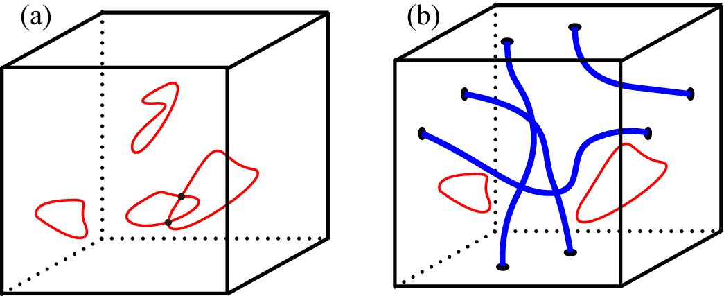
Figure 9(a) shows $T$ dependence of $\langle\bar{\phi}^{2}\rangle/L$. This quantity exhibits an anomaly at $T_{c}$; while $\langle\bar{\phi}^{2}\rangle/L$ is essentially zero below $T_{c}$, it becomes nonzero above $T_{c}$ in the thermodynamic limit. The behavior is similar to that in the classical dimer model, [25] which suggests that the high-$T$ paramagnetic phase has a Coulombic nature because of the constraints. The results indicate that the phase transition is characterized by the flux density. The flux $\phi_{i}^{\mu}$ corresponds to the winding number of the loop ${\cal C}_{i}$ along the vector $\bm{a}_{\mu}$. Hence, the result of $\langle\bar{\phi}^{2}\rangle/L$ in Fig. 9(a) indicates that, below $T_{c}$, the winding numbers vanish and only short loops are excited, as schematically shown in Fig. 10(a). On the other hand, the extended loops, which contribute to nonzero winding numbers, are generated above $T_{c}$ [see Fig. 10(b)]. Therefore, the phase transition can be characterized by the flux in terms of the loop model; namely, the zero (non-zero) flux phase is associated with the low-$T$ QSL (high-$T$ paramagnetic) phase.

Despite the lack of an appropriate order parameter, we analyze the critical behavior of the phase transition from the paramagnetic side by using $\langle\bar{\phi}^{2}\rangle$. Following the argument for the classical dimer model, [25] we assume the scaling $\langle\bar{\phi}^{2}\rangle/L=L^{-z}f(L^{1/\nu}(T-T_{c}))$, where $z$ is a scale exponent, $\nu$ is a critical exponent for correlation length, and $f(T)$ is a scaling function. Figure 9(b) shows $T$ dependence of $(\langle\bar{\phi}^{2}\rangle/L)/L^{-z}$ with $z=1$. The data for different $L$ cross with each other at the same point. This result indicates that the assumption $z=1$ is reasonable also for the present case. In addition, the scaling plot is shown in Fig. 9(c). Here, assuming $z=1$, we optimize $T_{c}$ and $\nu$ so that all the data collapse onto a single universal function. The analysis gives the estimates $T_{c}=1.925(1)$ and $\nu=0.60(5)$. The value of $T_{c}$ is fairly consistent with $T_{c}^{(L\to\infty)}$ in the inset of Fig. 4(b). In addition, the value of the critical exponent $\nu$ is consistent with that of the 3D Ising universality class. The values of $T_{c}$ and $\nu$ will be discussed in the next section IV.5.

The loop picture presented in Fig. 10 will be effective for understanding the nature of phase transition even in the parameter region apart from the limit of $J/J_{z}\to 0$ considered here. A finite $J$ brings about complicated interactions in the effective Hamiltonian from higher-order contributions in terms of $J$, which lead to interactions between loops. Nevertheless, the higher-order terms do not alter the loop-like structure of excited states, since it is a direct consequence of the local constraint of $K_{p}$ in Eq. (2) stemming from the basic spin algebra, which is imposed in the entire range of parameters. Given that the nature of transition is dominated by the global behavior of loop-like excitations in the limit of $J/J_{z}\to 0$ as sketched in Fig. 10, it is reasonable to expect that a similar transition takes place even at finite $J$. Such extension will be discussed elsewhere.

As described in Sec. II, the effective model in Eq. (3) is subject to both local and global constraints for the variables $B_{p}$. The local constraint restricts the excited states in the form of closed loops of $B_{p}=-1$ sites. It plays a decisive role on the finite-$T$ phase transition, as demonstrated in the previous sections. On the other hand, the role of the global constraints (i) and (ii) is not obvious. In this section, we examine it by studying the model with omitting the global constraints.

Figure 11(a) shows $T$ dependence of the specific heat divided by $T$ for the model in the absence of the global loops. In the MC simulation, we allow MC update by flipping a single six-site loop as well as the global update along an extended loop. Similar to the result in Fig. 4(b), the specific heat exhibits divergent behavior, although the peak values are slightly smaller than those in Fig. 4(b). The extrapolation of the peak temperature of $C$ to $L\to\infty$ gives an estimate of $T_{c}=1.920(2)$, as shown in the inset of Fig. 11(a). The estimate coincides well with that obtained in the inset of Fig. 4(b). Furthermore, we confirm that the scaling of the flux density $\langle\bar{\phi}^{2}\rangle/L$ also gives the same critical exponents, as in Sec. IV.4 (not shown). These results indicate that the global constraints (i) and (ii) are not relevant to the thermodynamics in the present effective model; the finite-$T$ phase transition takes place at the same $T_{c}$ with the same critical properties.

For further analysis from the viewpoint of the loop topology, let us introduce the parity variable $\eta=\eta_{x}\eta_{y}\eta_{z}$ for loop configurations. Here we define $\eta_{l}=(-1)^{n_{l}}$, where $n_{l}$ ($l=x,y,z$) is the number of extended loops in the $l$ direction. The parity $\eta$ distinguishes topologically different sectors of the loop configurations in the current model where loops are allowed to intersect with each other. In addition, $\eta$ is written by the flux of loops as $\eta=e^{i\pi\bar{\phi}^{2}}$. Note that $\eta$ is always +1 in the presence of the global constraints.

Figure 11(b) shows the numerical result for $T$ dependence of $\left<\eta\right>$. At high $T$, loop configurations with odd and even parity appear in the same weight, and hence, $\left<\eta\right>$ vanishes. On the other hand, below $T_{c}$, there are only short loops in the system as presented in Sec. IV.4, and hence, $\left<\eta\right>$ takes $+1$. In the vicinity of $T_{c}$, $\left<\eta\right>$ changes rapidly and the slope at $T_{c}$ increases with increasing the system size. The result implies that $\left<\eta\right>$ changes discontinuously from 0 to 1 at $T_{c}$ in the thermodynamic limit. Thus, this quantity appears to work as an order parameter for this phase transition, although the discontinuous jump looks incompatible with the continuous transition. As shown in Appendix B, however, the similar parity variable in a loop model on the 2D square lattice is indeed analytically shown to be a step function $\theta(\tilde{T}_{c}-T)$ in the thermodynamic limit, where $\tilde{T}_{c}$ is the critical temperature in the 2D loop model, though the transition is continuous in the Ising universality class.

Finally, we discuss a correspondence between our model and the Ising model. [26] If the global constraints (i) and (ii) are omitted, the effective loop model given by Eq. (3) becomes equivalent to the Ising model with NN interactions on the diamond lattice; by identifying the contributions from loops of length $\ell$ with the $\ell$-th order terms in the high-$T$ series expansion of the Ising model on the diamond lattice, the partition function of the loop model, $Z(\beta)$, is associated with that of the Ising model on a diamond lattice, $Z_{\rm Ising}(\beta)$, as

where $z=4$ is the coordination number of the diamond lattice. From this relation, we obtain the critical temperature for the present loop model as

where $T_{c}^{\prime}$ is the critical temperature of the Ising model on the diamond lattice. Using this relation and the previous result $T_{c}^{\prime}=2.7042(2)$, [27, 28] we obtain $T_{c}=1.9249(2)$. This value is consistent with our results for the effective model with and without global constraints. In addition, as discussed above, the critical exponent $\nu$ obtained from the scaling analysis of the flux density is also consistent with that of the 3D Ising universality class. These results confirm the validity of our characterization of the phase transition, although the correspondence to the Ising model is ensured only in the absence of the global constraints. The correspondence between the $Z_{2}$ spin liquid in a 3D toric code model and the 3D Ising model was also discussed in Ref. 18.

We note, however, that this correspondence does not describe the critical exponent of magnetic susceptibility $\chi^{zz}$ correctly. This is reasonable because $\chi^{zz}$ of the current 3D Kitaev model is defined through the correlation function of PS operators $\tau_{m}^{z}$, which does not show long-range ordering below $T_{c}$, in contrast to Ising spins in the 3D Ising model. To obtain the correct critical behavior of $\chi^{zz}$, we need the explicit calculations in terms of $\tau_{m}^{z}$, as discussed in Sec. IV.2.

References

- [1] L. Balents, Nature 464, 199 (2010).
- [2] Y. Shimizu, K. Miyagawa, K. Kanoda, M. Maesato, and G. Saito, Phys. Rev. Lett. 91, 107001 (2003).
- [3] S. Nakatsuji, Y. Nambu, H. Tonomura, O. Sakai, S. Jonas, C. Broholm, H. Tsunetsugu, Y. Qiu, and Y. Maeno, Science 309, 1697 (2005).
- [4] J. S. Helton, K. Matan, M. P. Shores, E. A. Nytko, B. M. Bartlett, Y. Yoshida, Y. Takano, A. Suslov, Y. Qiu, J.-H. Chung, D. G. Nocera, and Y. S. Lee, Phys. Rev. Lett. 98, 107204 (2007).
- [5] Y. Okamoto, M. Nohara, H. Aruga-Katori, and H. Takagi, Phys. Rev. Lett. 99, 137207 (2007).
- [6] M. Yamashita, N. Nakata, Y. Senshu, M. Nagata, H. M. Yamamoto, R. Kato, T. Shibauchi, and Y. Matsuda, Science 328, 1246 (2010).
- [7] D. S. Rokhsar and S. A. Kivelson, Phys. Rev. Lett. 61, 2376 (1988).
- [8] R. Moessner and S. L. Sondhi, Phys. Rev. Lett. 86, 1881 (2001).
- [9] A. Kitaev, Ann. Phys. 321, 2 (2006).
- [10] H. Morita, S. Watanabe, M. Imada, J. Phys. Soc. Jpn. 71, 2109 (2002).
- [11] S. Yan, D. A. Huse, and S. R. White, Science 332, 1173 (2011).
- [12] H.-C. Jiang, H. Yao, and L. Balents, Phys. Rev. B 86, 024424 (2012).
- [13] X. G. Wen, Quantum Field Theory of Many-Body Systems, (Oxford, New York, 2004).
- [14] G. Baskaran, S. Mandal, and R. Shankar, Phys. Rev. Lett. 98, 247201 (2007).
- [15] A. Hamma, R. Ionicioiu, and P. Zanardi, Phys. Rev. A 71, 022315 (2005).
- [16] C. Castelnovo and C. Chamon, Phys. Rev. B 76, 184442 (2007).
- [17] Z. Nussinov and G. Ortiz, Phys. Rev. B 77, 064302 (2008).
- [18] C. Castelnovo and C. Chamon, Phys. Rev. B 78, 155120 (2008).
- [19] S. Iblisdir, D. Pérez-Garciá, M. Aguado, and J. Pachos, Phys. Rev. B 79, 134303 (2009).
- [20] S. Iblisdir, D. Pérez-García, M. Aguado, and J. Pachos, Nucl. Phys. B 829, 401 (2010).
- [21] S. Mandal and N. Surendran, Phys. Rev. B 79, 024424 (2009).
- [22] S. Mandal and N. Surendran, arXiv:1101.3718.
- [23] F. G. Wang and D. P. Landau, Phys. Rev. Lett. 86, 2050 (2001).
- [24] J. Knolle, D. L. Kovrizhin, J. T. Chalker, and R. Moessner, arXiv:1308.4336.
- [25] F. Alet, G. Misguich, V. Pasquier, R. Moessner, and J. L. Jacobsen, Phys. Rev. Lett. 97, 030403 (2006).
- [26] Y. Kamiya, private communication.
- [27] J. W. Essam and M. F. Sykes, Physica 29, 378 (1963).
- [28] D. S. Gaunt and M. F. Sykes, J. Phys.: Math., Nucl. Gen. 6, 1517 (1973).
- [29] H. Takagi, private communication.
- [30] G. Jackeli and G. Khaliullin, Phys. Rev. Lett. 102, 017205 (2009).
- [31] E. K.-H. Lee, R. Schaffer, S. Bhattacharjee, and Y. B. Kim, Phys. Rev. B 89, 045117 (2014).
- [32] I. Kimchi, J. G. Analytis, A. Vishwanath, arXiv:1309.1171.
- [33] B. Kastening, Phys. Rev. E 66, 057103 (2002).
- [34] M. Wu and C. Hu, J. Phys. A. Math. Gen. 35, 5189 (2002).