Causal Domain Restriction for Eikonal Equations
Z. Clawson,22 2 Supported in part by the NSF through Graduate Research Fellowship and the 2010 REU at Cornell.88 8 Supported in part by the National Science Foundation grant DMS-1016150., A. Chacon,33 3 Supported in part by Alfred P. Sloan Foundation Graduate Fellowship.88 8 Supported in part by the National Science Foundation grant DMS-1016150., A. Vladimirsky88 8 Supported in part by the National Science Foundation grant DMS-1016150.
Center for Applied Mathematics and Department of Mathematics
Cornell University, Ithaca, NY 14853
Abstract
Many applications require efficient methods for solving continuous shortest path problems. Such paths can be viewed as characteristics of static Hamilton-Jacobi equations. Several fast numerical algorithms have been developed to solve such equations on the whole domain. In this paper we consider a somewhat different problem, where the solution is needed at one specific point, so we restrict the computations to a neighborhood of the characteristic. We explain how heuristic under/over-estimate functions can be used to obtain a causal domain restriction, significantly decreasing the computational work without sacrificing convergence under mesh refinement. The discussed techniques are inspired by an alternative version of the classical A* algorithm on graphs. We illustrate the advantages of our approach on continuous isotropic examples in 2D and 3D. We compare its efficiency and accuracy to previous domain restriction techniques. We also analyze the behavior of errors under the grid refinement and show how Lagrangian (Pontryagin’s Maximum Principle-based) computations can be used to enhance our method.
Section 1 Introduction
The Eikonal equation
| (1.1) |
arises naturally in many applications including continuous optimal path planning, computational geometry, photolithography, optics, shape from shading, and image processing [25]. One natural interpretation for the solution of (1.1) comes from isotropic time-optimal control problems. For a vehicle traveling through , describes the speed of travel and gives the exit time-penalty charged on . In this framework, is the value function; i.e., the minimum time to exit through if we start from a point . The characteristic curves of the PDE (1.1) define the optimal trajectories for the vehicle motion.
The value function is Lipschitz continuous, but generally is not smooth on . (The gradient of is undefined at all points for which an optimal trajectory is not unique.) Correspondingly, the PDE (1.1) typically does not have a smooth solution and admits infinitely many Lipschitz continuous weak solutions. Additional conditions introduced in [10] are used to restore the uniqueness: the viscosity solution is unique and coincides with the value function of the above control problem.
In the last 20 years, many fast numerical methods have been developed to solve (1.1) on the entire domain ; e.g., see [9, 24, 28, 32]. Many of these fast methods were inspired by classical label-correcting and label-setting algorithms on graphs; e.g., Sethian’s Fast Marching Method [24] mirrors the logic of the classical Dijkstra’s algorithm [11], which finds the minimum time to a target-node from every other node in the graph.
Our focus here is on a somewhat different situation, with the solution needed for one specific starting position only. On graphs, an A* modification of Dijkstra’s method [14] is widely used for similar single source / single target shortest path problems. There have been several prior attempts to extend A* techniques to algorithms for continuous optimal trajectory problems, but all of them have significant drawbacks: these methods either produce additional errors that do not vanish under numerical grid refinement [16, 17, 18, 19], or provide much more limited computational savings [12, 30, 31]. We believe that these disadvantages stem from an overly faithful mirroring of the “standard” A* on graphs. Our own approach is based on an alternative version of the A* algorithm [6] that has clear advantages in continuous optimal control problems. Numerical testing confirms that our method is both efficient (in terms of the percentage of domain restriction) and convergent under grid refinement.
We begin by reviewing two flavors of A* techniques on graphs in §2. We then describe the standard Fast Marching Method and its various A*-type modifications in §3. The numerical tests in §4 are used to compare the efficiency and accuracy of competing domain restriction techniques. We discuss the limitations of our approach and directions of future work in §5. The Appendix (§6) contains convergence analysis of the alternative A* under grid refinement, exploiting the probabilistic interpretation of the discretized equations.
Section 2 Domain restriction techniques on graphs
We start by defining the shortest path problem on a graph:
- •
A graph is defined by a set of nodes (vertices) and a set of directed arcs between these nodes.
- •
Along each arc we prescribe a transition time penalty , and assume if there is no transition from to .
- •
The sets of in-neighbors and out-neighbors of a node are respectively defined by
- •
Assume the graph is sparsely connected, i.e. for some fixed .
- •
The goal is to find the “value function” , defined as
Naturally, . On the rest of the graph, Bellman’s Optimality Principle [5] yields a coupled system of nonlinear equations:
| (2.1) |
Once the value function is known, an optimal path from any node to the target can be quickly recovered by recursively transitioning to the minimizing neighbor. A straight-forward iterative method for solving the system (2.1) would result in computational cost. Fortunately, this system is monotone causal: cannot depend on unless . This observation is the basis of the classical Dijkstra’s method, which recovers the value function on the entire graph in operations [11]. In Dijkstra’s method, all nodes are split into three classes: far (no value yet assigned), considered (assigned a tentative value), or accepted (assigned a permanent value).
Efficient implementations usually maintain the considered nodes as a binary heap, resulting in the term in the computational complexity.
Subsection 2.1 Estimates for “single-source / single-target” problems.
If we are only interested in an optimal path from a single starting location , Dijkstra’s method can be terminated as soon becomes accepted. (This changes the stopping criterion on line 4 of the pseudocode.) Other modifications of the algorithm can be introduced to further reduce the computational cost on this narrower problem. Consider a function
Any node lying on an optimal path from to must satisfy This provides an obvious relevance criterion, since for any that is not on an optimal path, . But since is generally unknown, all techniques for focusing computations on a neighborhood of this optimal path must instead rely on some “heuristic underestimate”
| (2.2) |
A stronger “consistency” requirement is often imposed instead:
| (2.3) |
(Note that is the maximum among all consistent heuristics that also satisfy .)
Such consistent underestimates are readily available for geometrically embedded graphs. Suppose and . If the “maximum speed” is such that for all and , then On a Cartesian grid-type graph, the Manhattan distance provides a better (tighter) underestimate For more general embedded graphs, a much better underestimate can be produced by “Landmark sampling” [13], but this requires additional precomputation and increases the memory footprint of the algorithm.
Some algorithms for this problem also rely on “heuristic overestimates”
An overestimate can be obtained as a total cost of any path from to or can also be found using landmark precomputations [13]. For structured geometrically embedded graphs, an analytic expression might also be available. E.g., on a Cartesian grid, if the “minimum speed” is such that , we can use
Subsection 2.2 A* Restriction Techniques
A* techniques restrict computations to potentially relevant nodes by limiting the number of nodes that become considered. A more accurate restricts a larger number of nodes from becoming considered, and if then only those nodes actually on the optimal path are ever accepted.
Standard A* (SA*). This version of A* is the one most often described in the literature [14]. Unlike in Dijkstra’s algorithm, the considered nodes are sorted and accepted based on values. This change affects line 1 in our pseudocode. The resulting algorithm typically accepts far fewer nodes before terminating: irrelevant nodes with large values might still become considered (if their neighbors are accepted) but will have lower priority and most of them will never become accepted themselves. Moreover, the consistency of ensures that accepted nodes receive exactly the same values as would have been produced by the original Dijkstra’s method. If actually depends on , then
guaranteeing that under SA* will not be accepted before .
Alternative A* (AA*). A less common variant of A* is described in [6]. Instead of favoring nodes with small , AA* simply ignores nodes that are clearly irrelevant. AA* relies on an underestimate (no longer required to satisfy (2.3)) and an additional upper bound (If an analytic or precomputed is available, we can take . But it is also possible to use the total cost of any feasible path from to .)
During Dijkstra’s algorithm, a node with (hence ) is surely not a part of the optimal path. Thus, to speed up Dijkstra’s algorithm, in AA* we still sort considered nodes based on values, but on line 1 we only mark considered if . Since the order of acceptance is the same, it is clear that AA* produces the same values as Dijkstra’s, but the efficiency of this technique is clearly influenced by the quality of (the smaller it is, the smaller is the number of considered nodes). This reliance on is a downside (since SA* only needs ), but has the advantage of making AA* also applicable to the label-correcting methods [6]. In section §3 we argue that AA* is also more suitable for continuous optimal control problems, in which an is often readily available.
AA* with Branch & Bound (B&B). In AA* remains static throughout the algorithm. The idea of Branch & Bound (B&B) is to dynamically decrease as we gain more information about the graph, making use of an overestimate function When accepting a node , we can also set
Exact estimates. Using “exact estimates” with A* would result in the maximal domain restriction. For both A* techniques, if and , the algorithm would only accept the nodes lying on an optimal path.
Section 3 Domain restriction in a continuous setting
The continuous time-optimal isotropic control problem deals with minimizing the time-to-exit for a vehicle, whose dynamics is governed by
| (3.1) |
Here is the starting position, is the control (i.e., the direction of motion) chosen at the time , is the vehicle’s time-dependent position, and is the spatially-dependent speed of motion. We will further assume the existence of two constants and such that holds For every time-dependent control we define the total time to the exit set as The value function is then naturally defined as
where is the exit-time penalty. Bellman’s optimality principle can be used to show that, if is a smooth function, it must satisfy a static Hamilton-Jacobi-Bellman PDE
with the natural boundary condition on . Using the isotropic nature of the dynamics, it is clear that the minimizer (i.e., the optimal initial direction of motion starting from ) is and the equation is equivalent to the Eikonal PDE (1.1). If the value function is not smooth, it can still be interpreted as a unique viscosity solution of this PDE [10].
Solving this PDE to recover the value function is the key idea of the dynamic programming. An analytic solution is usually unavailable, so numerical methods are needed to approximate . We use a first-order upwind discretization, whose monotonicity and consistency yield convergence to the viscosity solution [4]. To simplify the notation, we describe everything on a cartesian grid in , though higher dimensional generalizations are straightforward and similar discretizations are also available on simplicial meshes (e.g., [15, 26]; see also Figure 3). We will assume
- •
is discretized on a uniform grid with spacing .
- •
A gridpiont or node is denoted by with corresponding value , speed , and neighbors
This notation will be slightly abused (e.g., a gridpoint with a corresponding value , speed , etc…) whenever we emphasize the ordering of gridpoints rather than their geometric position.
- •
We will assume that is well-discretized on the grid, and we define the discretized exit-set In particular, the focus of our computational experiments will be on the case with the exit time-penalty . We note that does not have to be on the boundary of the square : if , then , and the border of the square is treated as an essentially outflow boundary. This corresponds to solving a constrained optimal control problem, with interpreted as a constrained viscosity solution [3].
We use the upwind finite differences [23] to approximate the derivatives of (1.1), resulting in a system of discretized equations. Using the standard four-point nearest-neighbors stencil at each , this results in:
| (3.2) |
If all the neighboring values are known, this is really a “quadratic equation in disguise” for . Letting and reduces (3.2) to
| (3.3) |
provided the solution satisfies ; otherwise we perform a one-sided update:
| (3.4) |
The system of discretized equations ((3.3) and (3.4) for all ) are monotone causal since needs only its smaller neighboring values to produce an update.
Sethian’s Fast Marching Method (FMM) [24] and another Dijkstra-like algorithm [28] due to Tsitsiklis take advantage of this monotone causality. FMM can be obtained from Dijkstra’s Method by changing the lines 3 and 7 to instead use the continuous update procedure (equations (3.3) and (3.4)). Similarly to Dijkstra’s method, FMM computes the value function on the entire grid in operations, where is the number of gridpoints. The key question is whether a significant reduction of computational cost is possible if we are only interested in an optimal trajectory starting from a single (pre-specified) source gridpoint .
Remark 3.0.
Restricting FMM to a smaller (relevant) subset of via A*-techniques is precisely the focus of this paper. But a legitimate related question is whether the dynamic programming approach is at all necessary when a single trajectory is all that we desire? In contrast to path planning on graphs, in the continuous control community, optimal trajectories for single source problems are typically recovered via Pontryagin Maximum Principle (PMP) [22]. This involves solving a two point boundary value problem for a state-costate system of ODEs, which in our context could be also derived as characteristic ODEs of the Eikonal PDE (1.1). One advantage of using PMP is that, unlike the dynamic programming, it does not suffer from the curse of dimensionality. In higher dimensions, solving a two-point boundary value problem is much more efficient than solving a PDE on the whole domain. Unfortunately, PMP is harder to apply if the speed function is not smooth. Even more unpleasantly, depending on the initial guess used to solve the two-point boundary value problem, that method often converges to locally optimal trajectories. In contrast, the dynamic programming always yields a globally optimal trajectory, and our approach can be used to lower its computational cost in higher dimensions. In fact, we show that both techniques can be used together, with a prior use of PMP improving the efficiency of A*, and A* verifying the global optimality of a PMP-produced trajectory.
Subsection 3.1 Domain restriction without heuristic underestimates.
Our algorithmic goal is to restrict FMM to a dynamically defined subset of the grid using underestimates of the cost-to-go and the previously computed values. This is the essence of several A*-type techniques compared in sections 3.2-3.5. But to motivate the discussion, we start by considering several simpler domain restriction techniques that do not involve the run-time use of underestimates.
First, we note that FMM can be terminated immediately after the gridpoint is accepted. In practice, this is unlikely to yield significant computational savings unless the set
is much smaller than the entire . (E.g., see the bolded level set in Figure 2A.)
Second, it is possible to use a “bi-directional FMM” (similar to the bi-directional Dijkstra’s [21]) by expanding two accepted clouds from the source and the target and stopping the process when they meet. The first gridpoint accepted in both clouds is guaranteed to lie on an -suboptimal trajectory from to . This approach is potentially much more efficient than the above. E.g., for a constant speed function , it cuts the -dimensional volume of the accepted set by the factor of ; see Figure 1.
Third, a different “elliptical restriction” approach is also applicable (and can be combined with the above bidirectional technique) whenever an overestimate for the minimal time from to is available.
Lemma 3.0.
Suppose the exit-set is given by a single target point , and is a known constant such that . Then the optimal trajectory satisfying (3.1) from is contained within the prolate spheroid (an ellipse in 2D) satisfying
| (3.5) |
Proof.
Let and be the distance and time along the optimal trajectory from to . Then
| (3.6) |
For any along the optimal trajectory we have
This inequality defines a prolate spheroid in and (3.5) immediately follows. ∎
Even if we are interested in an unconstrained problem (find the quickest trajectory in ), finite computer memory forces us to solve a state-constrained problem instead (find the quickest trajectory contained in ). The above Lemma is thus also useful to answer a related question: for which starting points does the -constrained problem have the same value function as the unconstrained? Clearly, for any point such that , enlarging the domain would not decrease .
Higher dimensional savings. Restricting computations to has an increasing effect in higher dimensions. The fraction of the volume of to the volume of the smallest bounding rectangular box is given by , which quickly approaches zero as grows. (E.g., in this fraction is , while in it is already ) If , the restriction to yields the computational savings of ; the savings are even higher if is any other box-rectangular domain fully containing .
Formulas for can be naturally obtained by computing (or bounding from above) the time along any feasible path from to On a convex domain , the most obvious choice is (i.e., follow the straight line from to at the minimum speed ). For problems with the unit speed of motion, , and the ellipse collapses to a straight line segment.
A more accurate overestimate can be obtained by computing the exact time needed to traverse that straight line trajectory:
For non-convex domains, a similar upper bound can be obtained by integrating the slowness along any feasible trajectory (e.g., the shortest -constrained path from to ).
Finally, we will also consider the third (“ideal”) option, with . While practically unattainable, is useful to illustrate the upper bound on efficiency of various domain restriction techniques. In practice, it can be approximated by using precomputed on a coarser grid or using the output of Pontryagin-Maximum-Principle-based computations (see the example in section 4.4). In the latter case, the techniques discussed in this paper can be viewed as a method for verifying the global optimality of a known locally-optimal trajectory. Figure 2A shows the -focused ellipses for a specific example with a highly oscillatory speed function.
| A | B |
|---|---|
Subsection 3.2 Dynamic domain restriction: underestimates and A*-techniques.
The previous subsection described a priori domain restriction techniques. Here, our goal is to further restrict the computations dynamically by using the solution already computed on parts of . The actual viscosity solution depends only on values along a characteristic (i.e., an optimal trajectory). Ideally, we would like to compute the numerical solution only for the gridpoints within an immediate neighborhood of that trajectory, potentially yielding a much greater speedup than the techniques described above.
Consider a function specifying the min-time from to . (It is easy to see that is also a viscosity solution of the Eikonal PDE (1.1), but with the different boundary condition .) We note that for all , and this becomes an equality if and only if lies on an optimal trajectory. (See the level sets of in Figure 2B.) Since is generally unknown, any practical restriction of computational domain will have to rely on an “admissible underestimate heuristic” , satisfying As we will see, tighter underestimates result in more efficient domain restrictions. Here we enumerate several natural heuristic underestimates:
- 1.
- 2.
- 3.
Landmarking-based heuristic [18, 19] is a continuous version of the landmarking technique on graphs [13]. This relies on pre-computing/storing the minimum time from every node to a number of “landmarks”; the triangle inequality is then used to obtain the lower bound . The high computational cost and memory footprint make this approach useful for repeated queries only. (I.e., only if the optimal trajectory problem has to be solved for many different pairs.)
- 4.
Higher-speed heuristic can be obtained by starting with a special speed-overestimate , such that the corresponding value function is known analytically, and then setting . (Note that (3.7) can be also derived this way by taking .) If the path-planning has to be performed for many different speed functions , the above approach can be useful even if has to be approximated numerically. One such example is included in section 4.4.
- 5.
Scaled “Oracle” heuristic [19] is defined as with . This is clearly not a practical underestimate, but a theoretical device useful in studying the accuracy/efficiency tradeoffs of various domain restriction techniques. Since is generally unavailable, our benchmarking relies on a numerical approximation; i.e., , where is (pre-)computed on the same grid .
The first of these (the Naïve heuristic) is a conservative underestimate that is cheaply available for all problems – including the situations with discontinuous speed functions and/or non-convex domains. The other underestimates are more expensive to produce, but usually result in a more significant domain restriction. Thus, their use is particularly justified when the same speed function is used repeatedly to solve numerous (single source / single target) problems.
We emphasize that this paper is in a sense “underestimate-neutral.” A good underestimate is obviously important, but our focus is on how it should be used rather than on how to build it.
Continuous A* Techniques. Both SA* and AA* algorithms on graphs may be easily adapted to the continuous setting using any of the above heuristics. Just like on graphs, SA*-FMM increases the “processing-priority” of nodes with low values, whereas our AA*-FMM avoids considering nodes guaranteed not to be a part of any -optimal trajectory. Each of these methods successfully restricts the computations, but with different trade-offs between the execution time, memory footprint, amount of restriction, and computational error.
Subsection 3.3 Prior work on SA*-FMM.
From the implementation standpoint, SA*-FMM is fairly straightforward. It requires modifying a single line 1 of FMM (see Dijkstra’s algorithm): accept the node with minimal . (Since is minimal along the -optimal trajectory, is used to indicate how close is to that trajectory.) However, the analysis of this method’s output is more subtle.
On graphs, the consistency of the heuristic underestimate (i.e., the condition (2.3)) guarantees that all SA*-accepted nodes receive the same values as would have been produced by Dijkstra’s. In contrast, SA*-FMM exhibits a performance tradeoff based on whether satisfies a more restrictive and stencil-dependent consistency condition (defined below). If is inconsistent, some of the gridpoints may be accepted prematurely, resulting in additional numerical errors. On the other hand, if is consistent, the efficiency of the domain restriction is significantly decreased, and this restricted domain does not shrink to zero volume as
The presence of additional errors might seem counterintuitive. After all, if an -optimal trajectory passes through some , then, for defined by formula (3.7),
guaranteeing that . Turning to numerical solutions, we would hope for the same argument to work for and , and indeed it does if is computed by a one-sided update formula (3.4). But for a first-order upwind discretization in , a generic gridpoint depends on other gridpoints that straddle ’s characteristic. To produce the same numerical values under SA*-FMM and FMM, we would need to know that whenever directly depends on .
Suppose there exists a constant such that
| (3.8) |
The proper ordering is then guaranteed provided the underestimate satisfies the consistency condition
| (3.9) |
which is easy to ensure by using the underestimate
Unfortunately, the condition (3.8) is stencil-dependent and in this section we explore its implications both on grids and triangular meshes; see Figure 3.
Suppose that ’s characteristic is straddled by and , where is the angle and is the angle between the characteristic and . Since for the Eikonal equation the characteristics coincide with gradient lines and our numerical approximation is piecewise linear, it is easy to show that11 1 We note that this observation was previously used in [29] to find the conditions for applicability of Dial-like algorithms.
The latter lower bound is actually sharp when the characteristic is parallel to and . This means that
- •
is the only consistent underestimate for stencil 3A (i.e., ). Thus, SA*-FMM will usually result in additional errors.
- •
for stencil 3B, becomes consistent for .
- •
for a local stencil used on a general triangular mesh (e.g., Figure 3D), if is an upper bound on angles present in the mesh, then becomes consistent for .
Interestingly, the importance of consistency conditions for SA*-FMM was only recently recognized in [30, 31], while all the prior versions treated this in an ad-hoc fashion. To summarize:
- •
[2005] Ferguson & Stentz [12] adapt D* algorithms to continuous optimal trajectory problems discretized on stencil 3B. They also introduce an SA*-type technique within D* to further improve the performance. The method relies on to ensure the right order of gridpoint processing, but the choice of is never explained explicitly.
- •
[2005, 2006, 2008] Peyré & Cohen [17, 18, 19] adapt SA* for FMM on stencil 3A using underestimates and . The authors acknowledge that their version of SA*-FMM produces additional errors and experimentally study the dependence of these errors on the tightness of underestimates. However, they do not analyze the behavior of errors under grid refinement.
- •
[2007] Pêtrès [16] defines an SA*-FMM variant on a stencil 3A with . A brief description of a bi-directional version of SA*-FMM is also included. Pêtrès acknowledges that, for large , the additional (SA*-induced) errors can be larger than discretization errors, but does not analyze how that ratio changes under grid refinement.
- •
[2011, 2012] Yershov & LaValle [30, 31] use FMM with acute triangular meshes as in [26] in , , and on two dimensional manifolds. Their problems of interest use on a domain with obstacles. The authors use SA*-FMM with and prove that guarantees absence of additional errors. The authors state that in their experiments SA*-FMM processed only 50% of the gridpoints processed by FMM.
Remark 3.0.
Every implementation of SA*-FMM also involves an “efficiency versus memory footprint” tradeoff. Since the binary heap of considered nodes is sorted based on , every heap-maintenance operation relies on availability of for many nodes on the heap. This happens whenever a far node becomes considered, or a considered node receives a smaller value or becomes accepted. If is re-computed each time it is needed (e.g., by (3.7)), this introduces a noticeable overhead to each heap operation. An alternative (to cache the first time it is computed for each considered node) is certainly more efficient, but significantly increases the memory footprint, particularly on larger grids and in higher-dimensional problems. In Section 4 we include the performance data for both of these approaches.
Subsection 3.4 Accuracy or efficiency?
The errors introduced by any A*-type restriction techniques are not very surprising once we recall that the numerical viscosity of the discretization results in a large domain of computational dependency for To formalize this argument, we will consider a dependency digraph built on the nodes of . For and , includes an arc if directly depends on ; i.e., if is needed to compute . We will say that depends on if there exists a path in from to . Due to the monotone causality of the upwinding discretization, this dependence implies ; thus, is acyclic and every path on it leads to . We will also use to denote the subset of reachable from .
Consider any domain restriction technique that results in accepting only nodes from some and produces some numerical approximation of the value function for each . If , we cannot expect to be the same as produced by FMM on the full . In other words, if we insist on avoiding any additional (restriction-induced) errors, this typically results in severe constraints on the efficiency of the domain restriction.
To illustrate this point, we consider a very simple problem with and in opposite corners of ; see Figure 4A. With the optimal trajectory from every starting position is just a straight line to . But it is easy to see that includes all nodes in ; thus, any restriction will result in . We emphasize that this phenomenon has nothing to do with the non-existence of consistent for the 4-point stencil discretization on a cartesian grid. Figure 4C shows an equivalent example on a regular triangular mesh. As explained in [30, 31], taking will ensure that is consistent for this problem and stencil. As a result, SA*-FMM will produce , but at the cost of accepting exactly the same set of nodes22 2 The computational savings of were reported in [30, 31] for on the domain with obstacles. Based on the above discussion, such savings are in fact highly dependent on the size of relative to the total number of meshpoints. This percentage is, in turn, defined by the type of the mesh and the positions of and relative to the obstacles. as FMM (i.e., ).
For these reasons, we believe that asking for on every fixed grid is unrealistic and makes the domain restriction much less efficient. A more attractive strategy is to ensure that is small relative to discretization errors and as This can be ensured provided covers a neighborhood of the -optimal trajectory and , the solution that FMM would have produced on . This is precisely what AA*-FMM does when used with an inconsistent ; on the other hand, the different order of acceptance under SA*-FMM typically results in and a lack of convergence (or a very slow convergence – see Section 4.1) under grid refinement.
Subsection 3.5 The new method: AA*-FMM
The AA* technique is also quite easy to use in the continuous setting as a modification of the standard FMM. Our current implementation is based on the upwind discretization (3.2) on a standard 4-point stencil, but the required FMM-changes would be the same for any other monotone-causal stencil (either on a grid or on a simplicial mesh). Similarly to a version of AA* for graphs:
- •
we rely on an overestimate of the time along the -optimal trajectory (see section 3.1);
- •
the considered nodes are still sorted by -values, and thus the underestimate does not have to satisfy any consistency conditions;
- •
we only mark a node as considered if it satisfies the “A* condition”
(3.10)
This simple criterion allows for AA* to be adapted to both label-setting and label-correcting methods. If satisfies the consistency condition (3.9), the values produced by AA*-FMM are also the same as those resulting from FMM, but on a smaller (accepted) subset of the grid . However, AA*-FMM can be also used even if does not satisfy (3.9), which results in additional errors but does not prevent the convergence to viscosity solution of the PDE under grid refinement.
To illustrate the efficiency of the AA*-type domain restrictions, we consider the boundaries of 3 sets:
| (3.11) |
All three are shown in Figure 5 for the example introduced in section 3.1. Both and are numerically approximated by FMM on the entire domain . The boundaries are shown by bold lines for and . The set corresponds to the ellipse defined for each specific . The set is roughly the set accepted by AA*-FMM with the specified and the underestimate . The set is the minimum part of the domain that AA*-FMM would have to accept with that even if we were to use the perfect If , then collapses to the optimal trajectory.
| A. Naïve | B. Integral-based | C. Exact |
|---|---|---|
This Figure also clearly demonstrates the importance of an accurate for the efficiency of the domain restriction in AA*-FMM. If the initial is not particularly tight, the performance can be further improved by decreasing dynamically in a Branch&Bound fashion. This approach relies on availability of a “heuristic overestimate” For a convex domain, our implementation uses an obvious (and cheaply computed) overestimate
| (3.12) |
which is consistent with our definition of in §3.1. Each time a gridpoint is accepted, this AA*BB-FMM algorithm attempts to decrease as follows:
| (3.13) |
A better can be obtained by numerically integrating the slowness along any feasible trajectory, or even using PMP-based techniques. Performing such computations for every accepted gridpoint would be clearly prohibitive, but using it every so often (in addition to the systematic use of formula (3.12)) could be a useful technique to investigate in the future.
Remark 3.0.
On graphs, using the exact “underestimate” simply resulted in accepting only those nodes that lie on the optimal path. In the continuous case, the optimal trajectory does not pass through every node it directly depends on. Even for a node immediately next to the optimal trajectory, if the underestimate is very accurate, this may cause the A* condition (3.10) to fail (resulting in never becoming considered). This situation rarely arises in practice – e.g., with this can happen only if is exact and the speed on some neighborhood of .
We have used two different approaches to address this issue:
- •
- •
Alternatively, if has not been accepted by the end of AA*-FMM, one can simply take . Since was obtained as a cost of some known trajectory, that trajectory is then declared optimal (at least for the current grid resolution).
Section 4 Numerical results
All algorithms were implemented in C++ and compiled with g++ version 4.2 on a Macbook Pro (4 GB RAM and an Intel Core i7 processor – four 2 GHz cores). To make the benchmarking results as compiler/platform-independent as possible, we have turned off all compiler optimizations (option -O0). For all of the 2D and 3D examples, is discretized by a uniform cartesian grid with gridpoints. To test the numerical approximation errors in distance computations (Section 4.1), we have used an analytical solution . In all other cases, the ‘ground truth’ was computed numerically by FMM on the full domain using the ‘highly’ refined grid:
| Dimension | Ground truth | Resolutions considered |
|---|---|---|
Accuracy metrics. Since we are interested in single-source / single-target problems, all accuracy metrics are based on comparing various numerical approximations and the true solution at a single point . As before, we use to denote the solution produced by FMM on the entire while denotes the solutions produced by the respective A*-modifications of FMM. We base our comparison on the following “relative errors” for each example:
Since the upwind discretization is convergent, and thus as . Correspondingly, a successful domain restriction should have (and thus ) as .
To measure the efficiency of the domain restriction, we also define
Underestimate functions. In all examples except for section 4.4, we rely on naïve and scaled-oracle heuristics (i.e., and ). We consider this sufficient since the accuracy of the AA* approach is really underestimate-neutral (though the efficiency is clearly dependent on both and ). We expect that the results based on any other heuristics (including those in [17, 18, 19]) will be qualitatively similar.
Subsection 4.1 Constant speed in 2D and 3D
In the constant speed case, all characteristics are straight lines and the the naïve heuristic coincides with the actual time-to-go (i.e., ). In this subsection we use the underestimate and place and at opposite corners of . Our goal is to test the effect of on the accuracy and efficiency for different grid resolutions . In testing AA*-FMM, we use , where with in 2D and in 3D. This ensures that AA*-FMM does not terminate before is accepted and also results in the set shrinking to a straight line as .
Figure 6 shows the level sets of computed by SA*-FMM and AA*-FMM on a 2D grid with and . The non-smoothness of the level-sets produced by SA*-FMM is due to the additional errors introduced by that method. For these errors also result in a larger – despite the fact that our AA*-FMM has a built-in “restriction slackness” (since ). Figure 7 shows as and vary. For , the errors produced by SA*-FMM are not only relatively large, but also do not decrease much under grid refinement. In contrast, the errors in AA*-FMM decrease quite rapidly even though the set is also shrinking as ; see also the convergence analysis in Section 6.
Since in this example , additional errors should result from any domain restriction. However, the finite-precision of the floating point arithmetic results in “zero domain restriction errors” (white spaces in Figure 7) for AA*-FMM even for many test runs where is partly truncated. E.g., see the case in Figures 6 and 7.
Contours of produced by A*-FMM using
|
SA* |
||||
|---|---|---|---|---|
| , | , | , | , | |
|
AA* |
||||
| , | , | , | , | |
2D constant speed: Error .
| SA* | AA* |
|---|---|
2D constant speed: Statistics.
| A. Time (sec) | B. Fraction | C. Error |
|---|---|---|
3D constant speed: Statistics.
| A. Time (sec) | B. Fraction | C. Error |
|---|---|---|
Subsection 4.2 Oscillatory speed function in 2D and 3D
For the next 2D example, we set and and consider a highly oscillatory speed
| (4.1) |
resulting in frequent directional changes along most optimal paths. We start by focusing on a scaled oracle heuristic with AA*-FMM also relying on . Figure 10 shows the level sets of numerical solutions obtained with . We note that the SA*-errors result in a significant distortion of the optimal trajectory (see the switch between and ).
| 2D sinusoid speed: Solutions with A* using | ||||||
|
SA* |
||||||
|---|---|---|---|---|---|---|
| , | , | , | , | , | , | |
|
AA* |
||||||
| , | , | , | , | , | , | |
Figure 11 compares the accuracy of these techniques for different pairs. Qualitatively the picture is largely the same as in Figure 7, but with two non-trivial differences. First, the ‘white block’ in the lower-left corner of the SA* plot indicates the lack of additional errors with and . Based on our computational experiments, this is an extremely rare situation – the only example we could find, where the entire is processed by SA*-FMM in the correct order despite the fact that the heuristic is inconsistent. Second, we observe that the AA*-FMM-generated errors are not always monotone decreasing in . E.g., the errors are present for , but not for , where the entire is accepted.
2D sinusoid speed: Error .
| SA* | AA* |
|---|---|
Since the oracle heuristic is generally unavailable, we now consider the accuracy/efficiency tradeoffs using the naïve heuristic and a realistically obtainable (but conservative) overestimate . Figure 12 shows that AA*-FMM yields comparable efficiency (despite accepting a larger part of the domain) while also ensuring since the entire is accepted.
2D sinusoid speed: Statistics.
| A. Time (sec) | B. Fraction | C. Error |
|---|---|---|
We also consider similar oscillatory examples in 3D with
| (4.2) |
for two amplitudes and . The source/target locations are and . Figure 13 shows the accuracy/efficiency data based on realistic and . The errors due to AA* are negligible compared to discretization errors, while the errors due to SA* are again quite noticeable and decrease much slower as .
3D sinusoid speed: Statistics.
| A. Time (sec) | B. Fraction | C. Error | |
|---|---|---|---|
|
|
|||
|
|
Subsection 4.3 Satellite image
The following path-planning example is borrowed from [17, 18, 19]. The grayscale intensities of a satellite photograph (Figure 14A) are imported into the range using Matlab’s imread() routine. For a given gridpoint assume that it falls into a pixel with grayscale value . This then defines the speed via rescaling:
This is the same intensity/speed mapping used in [19], but our experimental setup is slightly different:
- •
Unlike Peyré et al., we omit the pre-smoothing of the original image and simply downsample it to .
- •
- •
Figure 14B shows the level sets of the solution on the full domain, with and (using and ) shown in bold. (The set accepted by SA* is approximately the same as AA*.)
| A. Original image | B. PDE solution | C. Zoom on PDE solution |
|---|---|---|
 |
 |
This example illustrates the use of A*-techniques with a discontinuous speed function. The rather limited computational savings in 14B are clearly caused by the use of an “overly optimistic” . However, the lack of accuracy of this naive underestimate is not caused by any discontinuities in – instead it is simply a result of a large , with values much closer to on most of the domain.
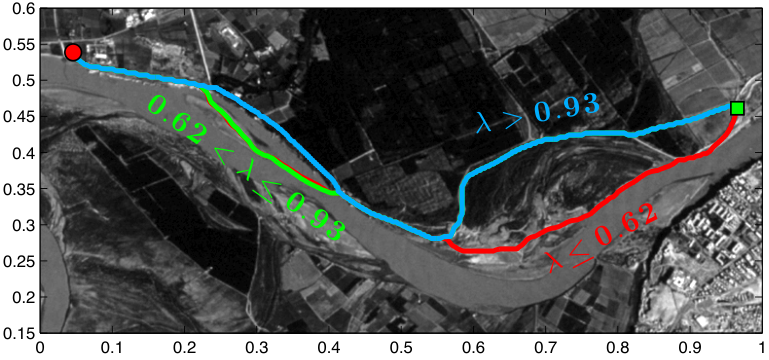
We now switch to “oracle tests” with and AA*-FMM relying on . Using this heuristic, the domain restriction becomes much more effective for both SA* and AA*. But since is close to a shockline, additional errors due to SA*-FMM are sufficiently large to change the optimal trajectory in several ways (see Figure 15A). In contrast, the errors from AA*-FMM are much smaller and the optimal trajectory remains the same for all .
| A. Different trajectories | B. Time | C. Error |
|---|---|---|
 |
Subsection 4.4 Replanning in a dynamic environment
Our final example illustrates several important points:
- 1.
The use of special/custom underestimate based on a related control problem.
- 2.
The optimal trajectory from a related control problem is valuable as an initial guess for the Pontryagin Maximum Principle (PMP).
- 3.
The PMP-computed trajectory is not necessarily globally optimal, but can be used to produce an accurate .
Here we will use a slightly more general setup where the task is to minimize the total cost (instead of considering only the time) to reach . Given a running cost function integrated along the trajectory and a speed , the value function now satisfies a different Eikonal PDE given by
| (4.3) |
Our specific problem is to find the “safest” trajectory in an adversarial environment, with higher on the parts of the domain more closely monitored by the adversary.
If we assume no prior information on enemy locations and monitoring patterns, it is natural to select , which implies that the quickest trajectory is in fact the safest. Consider the domain with the speed and running-cost defined by
The solution to this “no enemy observers” problem is shown in Figure 16C. Figure 16A shows the contours of with two locally optimal trajectories. The ‘upper’ solid trajectory is globally optimal and found by tracing the gradient of ; the ‘lower’ locally optimal trajectory is computed using PMP.
Our perception of the trajectory safety will change once we discover specific locations of enemy observers. For example, if we know that there are two observers located at and , we might encode this new information in the cost function:
The solution to (4.3) with speed and the above cost can be shown to satisfy (1.1) with . The contours of this new modified speed can be seen in Figure 16B with two “locally safest” trajectories that can be viewed as perturbations of the locally time-optimal paths from Figure 16A. Note that, because of the higher cost around , the ‘upper’ locally optimal trajectory is no longer globally optimal.
The full solution to the time-optimal problem becomes useful if we want to introduce A* techniques for all “multiple enemy observers” problems. Let be the minimum time to reach using the speed . Suppose that is pre-computed by FMM and stored for the entire . Returning to the problem with known observers, we may take since . The overestimate can be obtained by integrating along any feasible trajectory. If we use the globally time-optimal trajectory (the solid black curve in Figure 16A), this yields a good . An even better overestimate is obtained if we use the globally time-optimal trajectory as the initial guess for PMP, and then integrate along the resulting “locally safest” trajectory (the ‘upper’ black curve in Figure 16B).
Figure 16D shows the solution level sets for the “multiple enemy observers” problem together with boundaries of several computational sets. The bold black curve is , showing the part of accepted by FMM. The next (inward) bold curve is with – the boundary of a subset accepted by AA*-FMM. The final bold curve is with – this approximates the boundary of a subset accepted by SA*-FMM. (AA*-FMM would also restrict to the latter set, but only if we were lucky enough to start with corresponding to the ‘lower’ curve in Figure 16B).
Even though AA*-FMM computes the solution on a larger part of the domain, its computational efficiency is still comparable and the accuracy is superior to SA*-FMM. For example, with (using trial runs averaged for the time) we have
| Method | Time (seconds) | Ratio | Error |
|---|---|---|---|
| FMM | 0.02665 | 0.82 | 0 |
| SA*-FMM | 0.004950 | 0.130 | 0.02550 |
| AA*-FMM, | 0.0101 | 0.29 | |
| AA*-FMM, | 0.00526 | 0.14 | 0.00150 |
| A. Original speed | B. Modified speed | C. Original solution | D. Modified solution |
Section 5 Conclusions
We have described a new A*-type modification of the Fast Marching Method solving Eikonal equations for a ‘single source/target’ problem. Unlike the prior methods for this problem, which were developed to mirror in the ‘standard A*’ algorithm on graphs [14], our approach is based on a lesser known ‘alternative A*’ [6]. These prior SA*-FMM methods [12, 16, 17, 18, 19, 30, 31] either introduce additional errors that vanish slowly (if at all) under grid refinement, or must accept a much larger portion of the domain. In contrast, our AA*-FMM is able to significantly restrict computations, with any additional errors quickly decreasing under grid refinement.
One weakness of AA*-FMM is the reliance on an overestimate , especially when the feasibility of any trajectory is in question (e.g., in the presence of obstacles). A good can be also found from related control problems or based on Pontryagin Maximum Principle (PMP). Here we mention two more approaches not tested in the current paper:
- •
One can use , where and is the solution found by FMM on a much coarser grid.
- •
One can also use the output of SA*-FMM on the same grid with an aggressive/inconsistent , setting .
In the latter case, AA*-FMM should be viewed as a post-processing technique to improve the accuracy. This might seem superfluous: after all, PMP could also be applied using the output of SA*-FMM as an initial guess. But as we show in Figures 10 and 15, the errors from SA*-FMM are likely to result in PMP converging to some other (locally, rather than globally) optimal trajectory.
The effectiveness of the AA* domain restriction depends on the quality of and . If the initial is overly conservative, it can also be improved dynamically using the Branch & Bound techniques. No benchmarking results for the latter approach were included here for the sake of brevity.
We also list several desirable future extensions with significant impact on applications. First, AA* can be used instead of SA* within D* and E* path replanners [12, 20]. Second, the original AA* on graphs is applicable in both label-setting and label-correcting algorithms. It should not be hard to incorporate the same idea into other non-iterative and fast iterative methods for Hamilton-Jacobi PDEs. Our preliminary results for the Locking Sweeping Method [2] prove the feasibility of this approach. Third, since many gridpoints will never be used, allocating memory for the entire grid may be wasteful (particularly in high dimensions). One approach, described in [17, 18, 19], is to allocate gridpoints as needed and make use of a hash lookup table. Our current implementation of AA*-FMM does not use this idea, but we hope to explore it in the future. Finally, we note that all of the A* techniques can be also trivially extended to problems with a single-source and multiple targets. Similar underestimates can be also built for a moderately large set of sources (e.g., ).
The error analysis in the Appendix relies on a conjecture, which so far has been only proven for a linear advection equation. For the Eikonal case, we currently rely on experimental/numerical confirmation. Nevertheless, we believe that a similar approach will be also useful in analyzing errors in more general domain restriction problems; e.g., for the errors due to an “almost causal” domain decomposition in [7].
Aknowledgements. The authors would like to thank Slav Kirov for his contributions to the initial part of this project during the 2010-REU at Cornell University. We would also like to thank Gabriel Peyré for his input on the satellite image example used in Section 4.3.
Section 6 Appendix: Why does it converge?
If AA*-FMM is used with an inconsistent heuristic , the domain restriction usually affects the dependency graph (i.e., ), and the produced solution is larger than would result from running FMM on the full grid: . In this section we analyze why as .
We first note that the answer is simple if there exists an open set such that
- •
the -optimal trajectory lies in , and
- •
and all gridpoints falling into are accepted by AA*-FMM regardless of .
In this case, an -constrained viscosity solution will already yield the correct in the limit. In previous sections, we showed that such often arises because and/or are not tight. But if the over/underestimates also improve in quality as , then the AA*-FMM accepted region shrinks under grid refinement, and a more careful argument is needed to explain the convergence.
To address this, we compare solutions produced by the original FMM solving the same discretized system (3.2) but on different grid subsets and with different boundary conditions. For the rest of this section, we will not rely on the fact that is defined through AA*-FMM. As a benefit, our error analysis is also relevant for domain decomposition-based parallelizations of FMM; e.g., see [7].
Consider a restriction of FMM computations to any containing both and , and define the “restriction boundary” set For notational simplicity, we will assume that the -optimal trajectory is unique and that the upwind neighbors are uniquely defined for every gridpoint .
We will discuss the relationship between the following discretized solutions:
- •
As before, denotes the solution on the entire with the boundary condition .
- •
denotes the solution on with the same boundary condition . We can also interpret it as a solution on with and on . Recall that, if is defined as the set of nodes accepted by AA*-FMM, then this method also produces the same solution (i.e., on ).
- •
denotes the solution computed on with and the more general boundary conditions specified.
Observation 6.0.
The following properties are easy to verify based on the causality of (3.2):
- 1.
- 2.
- 3.
- 4.
Suppose is a constant such that . Then
- 5.
Suppose is the arclength of the shortest grid-aligned path within from to . Then
For any specific , if we define and choose this might result in . This “add-one-gridpoint-to-” procedure motivates our definition of sensitivity coefficients:
Due to the monotonicity of (3.2), and it is strictly positive if and only if .
Lemma 6.0.
The net effect of a domain restriction can be bounded from above using ’s even for a general set :
- 1.
If then
- 2.
If , then
Proof.
The upwind finite difference discretization (3.3) is equivalent to a semi-Lagrangian discretization:
| (6.1) |
Despite the very different Eulerian perspective and notation, (3.3) can be actually derived from Kuhn-Tucker optimality conditions for (6.1); see [28, 27, 29]. Moreover, the latter can be also viewed as the dynamic programming equation for a Stochastic Shortest Path Problem on the grid ; see [29] for a detailed discussion. In this interpretation, the transition from to the neighboring node (either or ) happens probabilistically, with respective probabilities and , and is the cost we incur for choosing this probability distribution. The process continues until we reach , and the goal is to select that minimizes the expected cumulative cost up to that termination. We note that, for , we have , and values on the rest of can be similarly computed using (6.1) recursively; see [8]. Moreover, if we start from and use the optimal “stochastic routing policy” , then can be naturally interpreted as a probability of passing through before arriving at .
Suppose now we use , but on a -restricted problem, starting from and terminating the process (+ paying the additional cost of ) if we transition into any before reaching . Denote by the expected total cost of using this policy and by the probability of reaching before termination. We first note that since some stochastic paths previously leading through are now removed due to an earlier entry to . Secondly, , since the latter is found by optimizing over all possible , including the restriction of . Thus,
which completes the proof of part 1. To prove part 2, select Since the exit-penalty is prohibitively high, the stochastic path starting from and using the optimal routing policy will avoid with probability 1. Thus, (see the last part of Observation 6), and using the above result
∎
Let be the distance from to the characteristic passing through (i.e., the -optimal trajectory).
Conjecture 6.0.
There exists a constant such that, for small enough , .
As of right now, we only have a rigorous proof of this statement for an upwind discretization of a constant-coefficient advection PDE [8, Chapter 4]. The same proof also covers the Eikonal equation when all characteristics are parallel, but this clearly does not hold for the case . Still, the numerical evidence (see Figure 17) indicates that this exponential decay is also present in the current context as well.
| A | B |
|---|---|
Theorem 6.1.
Proof.
We note that the -volume of the optimal-trajectory-centered -cylinder approaches zero, though the total number of gridpoints in grows as . For convenience, we also define which tends to as . If is the path length of the -optimal trajectory, then the number of gridpoints in is , where . Considering the shortest grid-aligned and -constrained path from any to , it is easy to show that is the upper bound for that path’s length. Thus, is an upper bound for . If Conjecture 6 holds, then asymptotically for all . By Lemma 6, is bound from above by which converges to under grid refinement. ∎
References
- [2] S. Bak, J. McLaughlin, & D. Renzi, Some Improvements for the Fast Sweeping Method, SIAM J. Sci. Comput., Vol. 32, No. 5, pp. 2853-2874, 2010.
- [3] M. Bardi and I. Capuzzo-Dolcetta, Optimal Control and Viscosity Solutions of Hamilton Jacobi-Bellman Equations, Birkhäuser, 1997.
- [4] G. Barles and P. E. Souganidis, Convergence of approximation schemes for fully nonlinear second order equations, Asymptot. Anal., 4:271-283, 1991.
- [5] R.E. Bellman, Dynamic Programming, Princeton University Press, Princeton, NJ, 1957.
- [6] D.P. Bertsekas, Dynamic Programming and Optimal Control, 2nd Edition, Volumes I and II, Athena Scientific, Boston, MA, 2001.
- [7] Cacace, S., Cristiani, E., Falcone, M., Picarelli, A. A patchy Dynamic Programming scheme for a class of Hamilton-Jacobi-Bellman equations, SIAM J. Sci. Comp. Vol. 34, No. 5, pp. A2625A2649, 2012.
- [8] A. Chacon, Eikonal Equations: new two-scale algorithms and error analysis, Ph.D. Thesis, Cornell University, 2013.
- [9] A. Chacon & A. Vladimirsky, Fast two-scale methods for Eikonal equations, SIAM J. on Scientific Computing, 34/2, 2012.
- [10] M.G. Crandall, P.-L. Lions, Viscosity solutions of Hamilton-Jacobi equations, Transactions of the American Mathematical Society, 277 (1), pp. 1–42,1983.
- [11] E.W. Dijkstra, A Note on Two Problems in Connexion with Graphs, Numerische Mathematik, Vol. 1, pp. 269-271, 1959.
- [12] D. Ferguson & A. Stentz, Field D*: An interpolation-based path planner and replanner, Proceedings of International Symposium on Robotics Research (ISRR), 2005.
- [13] A.V. Goldberg & C. Harrelson, Computing the Shortest Path: A* Search Meets Graph Theory, Technical Report, Microsoft Research, 2004.
- [14] P.E. Hart, N.J. Nilsson, & B. Raphael, A Formal Basis for the Heuristic Determination of Minimum Cost Paths, IEEE Transactions of Systems Science and Cybernetics, Vol. SSC-4, No. 2, pp. 100-107, 1968.
- [15] Kimmel, R. & Sethian, J.A., Fast Marching Methods on Triangulated Domains, Proc. Nat. Acad. Sci., 95, pp. 8341-8435, 1998.
- [16] C. Pêtrès, Trajectory Planning for Autonomous Underwater Vehicles, Heriot-Watt University, PhD Dissertation, 2007.
- [17] G. Peyré & L.D. Cohen, Heuristically Driven Front Propagation for Geodesic Paths Extraction, Proc. of VLSM ’05 (N. Paragios, O. D. Faugeras, T. Chan, C. Schnörr, eds.), Springer, vol. 3752, pp. 173-185, 2005.
- [18] G. Peyré & L.D. Cohen, Landmark-Based Geodesic Computation for Heuristically Driven Path Planning, Proc. of CVPR ’06, IEEE Computer Society, pp. 2229-2236, 2006
- [19] G. Peyré & L.D. Cohen, Heuristically Driven Front Propogation for Fast Geodesic Path Extraction, International Journal for Computational Vision and Biometrics Vol. 1, No. 1, pp. 55-67, 2008.
- [20] R. Philippsen, A Light Formulation of the E* Interpolated Path Replanner, Technical report, Autonomous Systems Lab, École Polytechnique Fédérale de Lausanne, 2006.
- [21] I. Pohl, Bi-directional Search, Machine Intelligence, vol. 6, eds. Meltzer and Michie, Edinburgh University Press, pp. 127-140, 1971.
- [22] L. S. Pontryagin, V. Boltyanskii, R. V. Gamkrelidze, & E. F. Mishenko, The Mathematical Theory of Optimal Processes, Wiley, 1962.
- [23] E. Rouy & A. Tourin, A Viscosity Solutions Approach to Shape-From-Shading, SIAM J. Num. Anal., 29, 3, pp. 867-884, 1992.
- [24] J.A. Sethian, A Fast Marching Level Set Method for Monotonically Advancing Fronts, Proc. Nat. Acad. Sci., 93, 4, pp. 1591–1595, February 1996.
- [25] J.A. Sethian, Level Set Methods and Fast Marching Methods: Evolving Interfaces in Computational Geometry, Fluid Mechanics, Computer Vision and Materials Sciences, Cambridge University Press, 1996.
- [26] J.A. Sethian & A. Vladimirsky, Fast Methods for the Eikonal and Related Hamilton–Jacobi Equations on Unstructured Meshes, Proc. Nat. Acad. Sci., 97, 11 (2000), pp. 5699–5703.
- [27] J.A. Sethian & A. Vladimirsky, Ordered Upwind Methods for Static Hamilton-Jacobi Equations: Theory & Algorithms, SIAM J. on Numerical Analysis 41, 1, pp. 325-363, 2003.
- [28] J.N. Tsitsiklis Efficient Algorithms for Globally Optimal Trajectories, IEEE Tran. Automatic Control, 40, pp. 1528–1538, 1995.
- [29] A. Vladimirsky, Label-setting methods for Multimode Stochastic Shortest Path problems on graphs, Mathematics of Operations Research 33(4), pp. 821-838, 2008.
- [30] D.S. Yershov, S.M. LaValle, Simplicial Dijkstra and A* Algorithms for Optimal Feedback Planning, in Proceedings IEEE/RSJ International Conference on Intelligent Robots and Systems (IROS), 2011.
- [31] D.S. Yershov, S.M. LaValle, Simplicial Dijkstra and A* Algorithms: From Graphs to Continuous Spaces, Advanced Robotics, Vol. 26, no. 17, pp. 2065-2085, 2012
- [32] H. Zhao, A Fast Sweeping Method for Eikonal Equations, Mathematics of Computation, Vol. 74, Num. 250, pp. 603-627, 2004.