Rigorous high-precision computation of the Hurwitz zeta function and its derivatives

For a precision of $P$ bits, we should choose $N\sim M\sim P$. A simple strategy is to do a binary search for an $N$ that makes the error bound small enough when $M=cN$ where $c\approx 1$. This is sufficient for our present purposes, but more sophisticated approaches are possible. In particular, for evaluation at large heights in the critical strip, $N$ should be larger than $M$.

Given complex balls for $s$ and $a$, and integers $N$ and $M$, we can evaluate the error bound (12) using ball arithmetic. The output is a power series with ball coefficients. The absolute value of each coefficient in this series should be added to the radius for the corresponding coefficient in $S+I+T\approx\zeta(s+x,a)$ at the end of the whole computation. If the assumptions that $\Re(a)+N>1$ and $\Re(s)+2M>1$ are not satisfied for all points in the balls $s$ and $a$, we set the error bounds for all coefficients to $+\infty$.

If we are computing $D$ derivatives and $D$ is large, the rising factorial $|(s+x)_{2M}|$ can be computed using binary splitting and the outer power series product in (12) can be done using fast polynomial multiplication, so that only $\tilde{O}(D+M)$ real number operations are required. Or, if $D$ is small and $M$ is large, $|(s+x)_{2M}|$ can be computed via the gamma function in time independent of $M$

As a power series, the power sum $S$ becomes $\sum_{k=0}^{N-1}(\sum_{i}c_{i}(k)x^{i})$ where the coefficients $c_{i}(k)$ are given by (10). For $i\geq 1$, the coefficients can be computed using the recurrence

If we are computing $D$ derivatives with a working precision of $P$ bits, the complexity of evaluating the power sum is $\tilde{O}(NPD)$, or $\tilde{O}(N^{2}D)$ if $N\sim P$. The computation is easy to parallelize by assigning a range of $k$ values to each thread (for large $D$, a more memory-efficient method is to assign a range of $i$ to each thread).

When evaluating the ordinary Riemann zeta function, i.e. when $a=1$, and we just want to compute a small number of derivatives, we can speed up the power sum a bit. Writing the sum as $\sum_{k=1}^{N}f(k)$, the terms $f(k)=k^{-(s+x)}$ are completely multiplicative, i.e. $f(k_{1}k_{2})=f(k_{1})f(k_{2})$. This means that we only need to evaluate $f(k)$ from scratch when $k$ is prime; when $k$ is composite, a single multiplication is sufficient.

This method has two drawbacks: we have to store previously computed terms, which requires $O(NPD)$ space, and the power series multiplication $f(k_{1})f(k_{2})$ becomes more expensive than evaluating $f(k_{1}k_{2})$ from scratch for large $D$. For both reasons, this method is only useful when $D$ is quite small (say $D\leq 4$).

We can avoid some redundant work by collecting multiples of small primes. For example, if we extract all powers of two, $\sum_{k=1}^{10}f(k)$ can be written as

This is a polynomial in $f(2)$ and can be evaluated from bottom to top using Horner’s rule while progressively adding the terms in the brackets. Asymptotically, this reduces the number of multiplications and the size of the tables by half. Algorithm 1 implements this trick, and requires about $\pi(N)\approx N/\log N$ evaluations of $f(k)$ and $N/2$ multiplications, at the expense of having to store about $N/6$ function values plus a table of divisors of about $N/2$ integers. Constructing the table of divisors using the sieve of Eratosthenes requires $O(N\log\log N)$ integer operations, but this cost is negligible when multiplications and $f(k)$ evaluations are expensive. One could also extract other powers besides 2 (for example powers of 3 and 5), but this gives diminishing returns.

Another trick that can save time at high precision is to avoid computing the logarithms of integers from scratch. If $q$ and $p$ are nearby integers (such as two consecutive primes) and we already know $\log(p)$, we can use the identity

and evaluate the inverse hyperbolic tangent by applying binary splitting to its Taylor series. This is not an asymptotic improvement over the best known algorithm for computing the logarithm (which uses the arithmetic-geometric mean), but likely faster in practice.

Except for the multiplication by Bernoulli numbers, the terms of the tail sum $T$ satisfy a simple (hypergeometric) recurrence relation. If we are computing $D$ derivatives with a working precision of $P$ bits, the complexity of evaluating the tail by repeated application of the recurrence relation is $\tilde{O}(MPD)$, or $\tilde{O}(P^{2}D)$ if $M\sim P$. We can do better if $D$ is large, using binary splitting (Algorithm 2).

If $D\sim M$, the complexity with binary splitting is only $\tilde{O}(PD)$, or softly optimal in the bit size of the output. A drawback is that the intermediate products increase the memory consumption.

The Bernoulli numbers can of course be cached for repeated evaluation of the zeta function, but computing them the first time can be a bottleneck at high precision, at least if done naively. The first $2M$ Bernoulli numbers can be computed in quasi-optimal time $\tilde{O}(M^{2})$, for example by using Newton iteration and fast polynomial multiplication to invert the power series $(e^{x}-1)/x$. For most practical purposes, simpler algorithms with a time complexity of $\tilde{O}(M^{3})$ are adequate, however. Various algorithms are discussed in [19]. An interesting alternative, used in unpublished work of Bloemen [3], is to compute $B_{n}$ via $\zeta(n)$ by direct approximation of the sum $\sum_{k=0}^{\infty}k^{-n}$, recycling the powers to process several $n$ simultaneously.

For $n\geq 1$, let $\rho_{n}$ denote the $n$-th smallest zero of $\zeta(s)$ with positive imaginary part. We assume that $\rho_{n}$ is simple and has real part $1/2$. Using Newton’s method, we can evaluate $\rho_{n}$ to high precision nearly as fast as we can evaluate $\zeta(s)$ for $s$ near $\rho_{n}$.

It is convenient to work with real numbers. The ordinate $t_{n}=\Im(\rho_{n})$ is a simple zero of the real-valued function $Z(t)=e^{i\theta(t)}\zeta(1/2+it)$ where

We assume that we are given an isolating ball $B_{0}=[m_{0}-\varepsilon_{0},m_{0}+\varepsilon_{0}]$ such that $t_{n}\in B_{0}$ and ${t_{m}\not\in B_{0}},{m\neq n}$, and wish to compute $t_{n}$ to high precision (finding such a ball for a given $n$ is an interesting problem, but we do not consider it here).

Newton’s method maps an approximation $z_{n}$ of a root of a real analytic function $f(z)$ to a new approximation $z_{n+1}$ via $z_{n+1}=z_{n}-f(z_{n})/f^{\prime}(z_{n})$. Using Taylor’s theorem, the error can be shown to satisfy

for some $\xi_{n}$ between $z_{n}$ and the root.

As a setup step, we evaluate $Z(s),Z^{\prime}(s),Z^{\prime\prime}(s)$ (simultaneously using power series arithmetic) at $s=B_{0}$, and compute

This only needs to be done at low precision.

Starting from an input ball $B_{k}=[m_{k}-\varepsilon_{k},m_{k}+\varepsilon_{k}]$, one step with Newton’s method gives an output ball $B_{k+1}=[m_{k+1}-\varepsilon_{k+1},m_{k+1}+\varepsilon_{k+1}]$. The updated midpoint is given by

where we evaluate $Z(m_{k})$ and $Z^{\prime}(m_{k})$ simultaneously using power series arithmetic. The updated radius is given by $\varepsilon_{k+1}=\varepsilon^{\prime}_{k+1}+C\varepsilon_{k}^{2}$ where $\varepsilon^{\prime}_{k+1}$ is the numerical error (or a bound thereof) resulting from evaluating (15) using finite-precision arithmetic. The new ball is valid as long as $B_{k+1}\subseteq B_{k}$ (if this does not hold, the algorithm fails and we need to start with a better $B_{0}$ or increase the working precision).

For best performance, the evaluation precision should be chosen so that $\varepsilon^{\prime}_{k+1}\approx C\varepsilon_{k}^{2}$. In other words, for a target accuracy of $p$ bits, the evaluations should be done at $\ldots,p/4,p/2,p$ bits, plus some guard bits.

As a benchmark problem, we compute an approximation $\tilde{\rho}_{1}$ of the first nontrivial zero $\rho_{1}\approx 1/2+14.1347251417i$ and then evaluate $\zeta(\tilde{\rho}_{1})$ to the same precision. We compare our implementation of the zeta function and the root-refinement algorithm described above (starting from a double-precision isolating ball) with the zetazero and zeta functions provided in mpmath version 0.17 in Sage 5.10 [31] and the ZetaZero and Zeta functions provided in Mathematica 9.0. The results of this benchmark are shown in Table 1. At 10000 digits, our code for computing the zero is about two orders of magnitude faster than the other systems, and the subsequent single zeta evaluation is about one order of magnitude faster.

We have computed $\rho_{1}$ to 303000 digits, or slightly more than one million bits, which appears to be a record (a 20000-digit value is given in [27]). The computation used up to 62 GiB of memory for the sieved power sum and the storage of Bernoulli numbers up to $B_{325328}$ (to attain even higher precision, the memory usage could be reduced by evaluating the power sum without sieving, perhaps using several CPUs in parallel, and not caching Bernoulli numbers).

Riemann’s function $\xi(s)=\frac{1}{2}s(s-1)\pi^{-s/2}\Gamma(s/2)\zeta(s)$ satisfies the symmetric functional equation $\xi(s)=\xi(1-s)$. The coefficients $\{\lambda_{n}\}_{n=1}^{\infty}$ defined by

were introduced by Keiper [22], who noted that the truth of the Riemann hypothesis would imply that $\lambda_{n}>0$ for all $n>0$. In fact, Keiper observed that if one makes an assumption about the distribution of the zeros of $\zeta(s)$ that is even stronger than the Riemann hypothesis, the coefficients $\lambda_{n}$ should behave as

Keiper presented numerical evidence for this conjecture by computing $\lambda_{n}$ up to $n=7000$, showing that the approximation error appears to fluctuate increasingly close to zero. Some years later, Li proved [25] that the Riemann hypothesis actually is equivalent to the positivity of $\lambda_{n}$ for all $n>0$ (this reformulation of the Riemann hypothesis is known as Li’s criterion). Recently, Arias de Reyna has proved that a certain precise statement of (16) also is equivalent to the Riemann hypothesis [10].

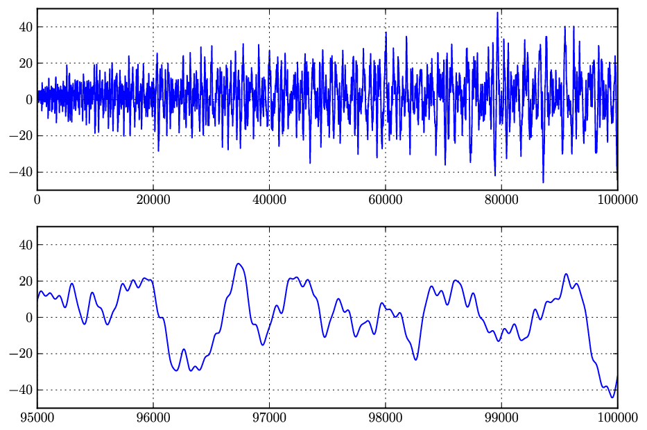
A computation of the Keiper-Li coefficients up to $n=100000$ shows agreement with Keiper’s conjecture (and the Riemann hypothesis), as illustrated in Figure 1. We obtain $\lambda_{100000}=4.62580782406902231409416038\ldots$ (plus about 2900 more accurate digits), whereas (16) gives $\lambda_{100000}\approx 4.626132$. Empirically, we need a working precision of about $n$ bits to determine $\lambda_{n}$ accurately. A breakdown of the computation time to determine the signs of $\lambda_{n}$ up to $n=1000$, $10000$ and $100000$ is shown in Table 2.

Our computation of the Keiper-Li coefficients uses the formula

which we evaluate at $s=x\in\mathbb{R}[[x]]$. This arrangement of the terms avoids singularities and branch cuts at the expansion point. We carry out the following steps (plus some more trivial operations):

1. 1.

   Computing the series expansion of $\zeta(s)$ at $s=0$.

2. 2.

   Computing the logarithm of a power series, i.e. $\log f(x)=\int f^{\prime}(x)/f(x)dx$.

3. 3.

   Computing the series expansion of $\log\Gamma(s)$ at $s=1$, i.e. computing $\gamma,\zeta(2),\zeta(3),\zeta(4),\ldots$.

4. 4.

   Finally, right-composing by $x/(x-1)$ to obtain the Keiper-Li coefficients.

Step 2 requires $O(M(n))$ arithmetic operations on real numbers. We use a hybrid algorithm to compute the integer zeta values in step 3; the details are beyond the scope of the present paper.

There is a very fast way to perform step 4. For $f=\sum_{k=0}^{\infty}a_{k}x^{k}\in\mathbb{C}[[x]]$, the binomial (or Euler) transform $T\colon\mathbb{C}[[x]]\to\mathbb{C}[[x]]$ is defined by

We have

If $B\colon\mathbb{C}[[x]]\to\mathbb{C}[[x]]$ denotes the Borel transform

then (see [16]) $T[f(x)]=B^{-1}[e^{x}B[f(-x)]]$. This identity gives an algorithm for evaluating the composition which requires only $M(n)+O(n)$ coefficient operations where $M(n)=\tilde{O}(n)$ is the operation complexity of polynomial multiplication. Moreover, this algorithm is numerically stable (in the sense that it does not significantly increase errors from the input when using ball arithmetic), provided that a numerically stable polynomial multiplication algorithm is used.

The composition could also be carried out using various generic algorithms for composition of power series. We tested three other algorithms, and found them to perform much worse:

• •

  Horner’s rule is slow (requiring about $nM(n)$ operations) and is numerically unsatisfactory in the sense that it gives extremely poor error bounds with ball arithmetic.

• •

  The Brent-Kung algorithm based on matrix multiplication [8] turns out to give adequate error bounds, but uses about $O(n^{1/2}M(n)+n^{2})$ operations which still is expensive for large $n$.

• •

  We also tried binary splitting: to evaluate $f(p/q)$ where $f$ is a power series and $p$ and $q$ are polynomials, we recursively split the evaluation in half and keep numerator and denominator polynomials separated. In the end, we perform a single power series division. This only costs $O(M(n)\log n)$ operations, but turns out to be numerically unstable. It would be of independent interest to investigate whether this algorithm can be modified to avoid the stability problem.

References

- [1] D. H. Bailey and J. M. Borwein. Experimental mathematics: recent developments and future outlook. In B. Engquist, W. Schmid, and P. W. Michor, editors, Mathematics Unlimited – 2001 and Beyond, pages 51–66. Springer, 2000.
- [2] D. J. Bernstein. Fast multiplication and its applications. Algorithmic Number Theory, 44:325–384, 2008.
- [3] R. Bloemen. Even faster calculation!, 2009. http://remcobloemen.nl/2009/11/even-faster-zeta-calculation.html.
- [4] A. I. Bogolubsky and S. L. Skorokhodov. Fast evaluation of the hypergeometric function at the singular point by means of the Hurwitz zeta function . Programming and Computer Software, 32(3):145–153, 2006.
- [5] J. Bohman and C-E. Fröberg. The Stieltjes function – definition and properties. Mathematics of Computation, 51(183):281–289, 1988.
- [6] J. M. Borwein, D. M. Bradley, and R. E. Crandall. Computational strategies for the Riemann zeta function. Journal of Computational and Applied Mathematics, 121:247–296, 2000.
- [7] P. Borwein. An efficient algorithm for the Riemann zeta function. Canadian Mathematical Society Conference Proceedings, 27:29–34, 2000.
- [8] R. P. Brent and H. T. Kung. Fast algorithms for manipulating formal power series. Journal of the ACM, 25(4):581–595, 1978.
- [9] M. W. Coffey. An efficient algorithm for the Hurwitz zeta and related functions. Journal of Computational and Applied Mathematics, 225(2):338–346, 2009.
- [10] J. Arias de Reyna. Asymptotics of Keiper-Li coefficients. Functiones et Approximatio Commentarii Mathematici, 45(1):7–21, 2011.
- [11] The GMP development team. GMP: The GNU multiple precision arithmetic library. http://www.gmplib.org.
- [12] The MPIR development team. MPIR: Multiple Precision Integers and Rationals. http://www.mpir.org.
- [13] H. M. Edwards. Riemann’s zeta function. Academic Press, 1974.
- [14] P. Flajolet and I. Vardi. Zeta function expansions of classical constants. Unpublished manuscript, http://algo.inria.fr/flajolet/Publications/landau.ps, 1996.
- [15] L. Fousse, G. Hanrot, V. Lefèvre, P. Pélissier, and P. Zimmermann. MPFR: A multiple-precision binary floating-point library with correct rounding. ACM Transactions on Mathematical Software, 33(2):13:1–13:15, June 2007. http://mpfr.org.
- [16] H. Gould. Series transformations for finding recurrences for sequences. Fibonacci Quarterly, 28:166–171, 1990.
- [17] B. Haible and T. Papanikolaou. Fast multiprecision evaluation of series of rational numbers. In J. P. Buhler, editor, Algorithmic Number Theory: Third International Symposium, volume 1423, pages 338–350. Springer, 1998.
- [18] W. B. Hart. Fast Library for Number Theory: An Introduction. In Proceedings of the Third international congress conference on Mathematical software, ICMS’10, pages 88–91, Berlin, Heidelberg, 2010. Springer-Verlag. http://flintlib.org.
- [19] D. Harvey and R. P. Brent. Fast computation of Bernoulli, tangent and secant numbers, 2011. http://arxiv.org/abs/1108.0286.
- [20] G. Hiary. Fast methods to compute the Riemann zeta function. Annals of mathematics, 174:891–946, 2011.
- [21] Wofram Research Inc. Some notes on internal implementation (section of the online documentation for Mathematica 9.0). http://reference.wolfram.com/mathematica/tutorial/SomeNotesOnInternalIm%plementation.html, 2013.
- [22] J. B. Keiper. Power series expansions of Riemann’s function. Mathematics of Computation, 58(198):765–773, 1992.
- [23] C. Knessl and M. Coffey. An effective asymptotic formula for the Stieltjes constants. Mathematics of Computation, 80(273):379–386, 2011.
- [24] R. Kreminski. Newton-Cotes integration for approximating Stieltjes (generalized Euler) constants. Mathematics of Computation, 72(243):1379–1397, 2003.
- [25] X-J. Li. The positivity of a sequence of numbers and the Riemann Hypothesis. Journal of Number Theory, 65(2):325–333, 1997.
- [26] Y. Matiyasevich. An artless method for calculating approximate values of zeros of Riemann’s zeta function, 2012. http://logic.pdmi.ras.ru/~yumat/personaljournal/artlessmethod/.
- [27] Y. Matiyasevich and G. Beliakov. Zeroes of Riemann’s zeta function on the critical line with 20000 decimal digits accuracy, 2011. http://dro.deakin.edu.au/view/DU:30051725?print_friendly=true.
- [28] A. M. Odlyzko and A. Schönhage. Fast algorithms for multiple evaluations of the Riemann zeta function. Transactions of the American Mathematical Society, 309(2):797–809, 1988.
- [29] F. W. J. Olver. Asymptotics and Special Functions. A K Peters, Wellesley, MA, 1997.
- [30] Y.-F.S Pétermann and J-L. Rémy. Arbitrary precision error analysis for computing with the Cohen-Olivier algorithm: complete description of the real case and preliminary report on the general case. Rapport de recherche RR-5852, INRIA, 2006.
- [31] W. A. Stein et al. Sage Mathematics Software. The Sage Development Team, 2013. http://www.sagemath.org.
- [32] J. van der Hoeven. Making fast multiplication of polynomials numerically stable. Technical Report 2008-02, Université Paris-Sud, Orsay, France, 2008.
- [33] J. van der Hoeven. Ball arithmetic. Technical report, HAL, 2009. http://hal.archives-ouvertes.fr/hal-00432152/fr/.
- [34] L. Vepštas. An efficient algorithm for accelerating the convergence of oscillatory series, useful for computing the polylogarithm and Hurwitz zeta functions. Numerical Algorithms, 47(3):211–252, 2008.