Maximizing submodular functions
using probabilistic graphical models
Abstract
We consider the problem of maximizing submodular functions; while this problem is known to be NP-hard, several numerically efficient local search techniques with approximation guarantees are available. In this paper, we propose a novel convex relaxation which is based on the relationship between submodular functions, entropies and probabilistic graphical models. In a graphical model, the entropy of the joint distribution decomposes as a sum of marginal entropies of subsets of variables; moreover, for any distribution, the entropy of the closest distribution factorizing in the graphical model provides an bound on the entropy. For directed graphical models, this last property turns out to be a direct consequence of the submodularity of the entropy function, and allows the generalization of graphical-model-based upper bounds to any submodular functions. These upper bounds may then be jointly maximized with respect to a set, while minimized with respect to the graph, leading to a convex variational inference scheme for maximizing submodular functions, based on outer approximations of the marginal polytope and maximum likelihood bounded treewidth structures. By considering graphs of increasing treewidths, we may then explore the trade-off between computational complexity and tightness of the relaxation. We also present extensions to constrained problems and maximizing the difference of submodular functions, which include all possible set functions.
1 Introduction
Optimizing submodular functions has been an active area of research with applications in graph-cut-based image segmentation [4], sensor placement [17], or document summarization [20]. A set function is a function defined on the power set of a certain set . It is submodular if and only if for all , . Equivalently, these functions also admit the diminishing returns property, i.e., the marginal cost of an element in the context of a smaller set is more than its cost in the context of a larger set. Classical examples of such functions are entropy, mutual information, cut functions, and covering functions—see further examples in [11, 1].
Submodular functions form an interesting class of discrete functions because minimizing a submodular function can be done in polynomial time [11], while maximization, although NP-hard, admits constant factor approximation algorithms [25]. In this paper, our ultimate goal is to provide the first (to the best of our knowledge) generic convex relaxation of submodular function maximization, with a hierarchy of complexities related to known combinatorial hierarchies such as the Sherali-Adams hierarchy [26]. Beyond the graphical model tools that we are going to develop, having convex relaxations may be interesting for several reasons: (1) they can lead to better solutions, (2) they provide online bounds that may be used within branch-and-bound optimization and (3) they ease the use of such combinatorial optimization problems within structured prediction framework [30].
Feige et al. [10] proposed constant factor approximation algorithms for maximizing non-negative submodular functions. They provide a randomized local search technique which optimizes a multilinear auxiliary function with some approximation guarantees. Buchbinder et al. [5] proposed a ramdomized -approximation algorithm to maximize non-negative submodular functions. They also use a randomized local search to remove or add an element for the existing set under consideration in each iteration of the algorithm. However, these methods only consider unconstrained submodular maximization.
Recent works also consider maximization of non-negative submodular functions [31] with packing-type constraints such as knapsack constraints, matroid constraints and their intersections with -approximation guarentee with respect to the best integer solution on the matroid polytope. They consider an extreme point of the polytope and provide a technique to replace an element of the extreme point fractionally using linear optimization. Iyer et al. [14] proposed semi-differentials, discrete equivalent of gradients, to define linear bounds on submodular functions. The approximations thus obtained are optimized using CCCP-like [35] procedures.
Among submodular functions, entropies have been particularly well-studied. Given , we consider random variables (jointly referred to as ) where denotes the domain of the random variables. In this paper, we consider only discrete-valued distributions but all our concepts extend to differential entropies [9]. The joint entropy of the variables indexed by is equal to , where denotes the marginal distribution of the random variables belonging to the set . Discrete entropies are known to be non-decreasing submodular set functions–the submodularity being a consequence of the data-processing inequality [9]. They are also known to be a strict subset of non-decreasing submodular set functions, i.e., when , there exist set functions which are non-decreasing and submodular but not entropies [36].
The relationship between submodularity and entropies has classically been useful in various probabilistic modeling tasks involving entropies, e.g., for proposing approximate algorithms for learning bounded treewidth graphical models [22, 6], for learning naive Bayes models [16] or for discriminative structure learning [23]. In this paper, we consider transfers in the opposite direction and will extend notions which are usually linked with entropies to all submodular functions. This will be achieved through probabilistic graphical models.
A joint distribution on is said to factorize in a graph if and only the distribution has a factored form where each factor depends only on a smaller subset of variables, a clique (for undirected graphs) or a node with its parents (for directed graphs). See, e.g., [15, 3, 21]. In decomposable undirected and directed graphical models, the entropy of the joint distribution decomposes as a sum of marginal entropies of subsets of variables. Moreover, for any distribution, the entropy of the closest distribution factorizing in the graphical model provides an bound on the entropy. For directed graphical models, this last property turns out to be a direct consequence of the submodularity of the entropy function. We leverage this property to propose a graphical-model-based upper bound for a general class of submodular functions, thus providing a flexible way of defining upper bounds for any submodular function. We study these bounds and their properties in detail in Section 2.
Given a bound on that depends on a free parameter (the graph structure), we may bring to bear variational inference techniques [34]: we will try to maximize with respect to while minimizing with respect to the variational parameter . In order to cast this variational problem as a convex optimization problem, we will use outer approximations of the marginal polytope [34] and inner approximations of the hypertree polytope that represents bounded treewidth graph structures [22, 18]. We obtain in Section 4 a saddle point problem which can be solved in polynomial time.
In this paper, we make the following contributions:
- –
- –
In Section 4, we propose an algorithm to maximize submodular functions by maximizing the bound with respect to while minimizing with respect to the graph , leading to a convex variational method based on outer approximation of the marginal polytope [34] and inner approximation of the hypertree polytope.
- –
In Section 5, we propose extensions to constrained problems and maximizing the difference of submodular functions, which include all possible set functions.
- –
We illustrate our results on small-scale experiments in Section 6.
Notations. Throughout this paper, we consider a submodular function defined on the set such that . We use the following definition of submodularity through the diminishing return property: . The main results of the paper do not require additional concepts; in Section 5, we will need additional concepts such as Lovász extensions and base polytopes, which will be presented there. For more details see [1, 11].
2 Directed graphical models
In this section, we first review the theory of directed graphical models (for more details, see [15, 3, 21]), and highlight the properties of entropies, which will allow us to define our bounds.
2.1 Probabilistic directed graphical models
A joint distribution on is said to factorize in the directed acyclic graph (DAG) if and only if the distribution may be written as , where is the set of parents of node in . The entropy may then be written as
When does not factorize in , we define as (and refer to it as the projection of onto ) the distribution which is closest (in Kullback-Leibler divergence) to that factorizes in . Since maximum-likelihood parameter estimation decouples in directed graphical models, a short calculation shows that and that the KL-divergence is equal to . Thus, the quantity is always an bound on and is equal to if and only if factorizes in .
Marginalization. Given a graph , we define by the graph restricted to i.e., . In general, if factorizes in , does not factorize in , unless is an ancestral set, i.e., all parents of all elements of are in (in other words, we may recursively remove leaf nodes and preserves the factorization). In the following, we denote by the entropy of the projection of onto . Note that is different in general from (which is the marginal of the projection of onto ). We have
| (1) |
From properties of entropies and graphical models, we have for any DAG and set . We show in the next section that this property turns out to be a consequence of submodularity.
Structure learning. Although we will not use structure learning in this paper, it is worth noting that several entropy-based approaches have been considered for finding the best possible graph (with some constraints) given a probability distribution. They are based on the decomposition of entropies and local search (see, e.g., [7] and references therein).
2.2 Bounds on submodular functions
Given a submodular function such that , following Eq. (1), we define as
| (2) |
When is an entropy function, is the entropy of the distribution closest to the distribution of that factorizes in (which is not equal to the marginal entropy on of the closest distribution that factorizes in ). We now show that bounds and that the bound is tight for some subsets of (see all additional proofs in the supplementary material).
Proposition 1 (Upper bound)
Let be a submodular function and a directed acyclic graph. The function defined in Eq. (2) bounds , i.e., for all , .
Proof Without loss of generality, we assume that is the topological ordering (i.e., ), without loss of generality. For all ,
Proposition 2 (Tightness of the bound)
For any element, , and any subset of , i.e., , .
Note that a corollary of Prop. 2 is that the bound is tight on all singletons (by considering ). This implies that any modular properties of are preserved (and this notably implies that without loss of generality, we may consider only non-decreasing functions). The bound also has other interesting monotonicity properties, which we now show.
Proposition 3 (Monotonicity of bounds - I)
If is a subgraph of the DAG , then , i.e., for all , .
The following proposition shows that the difference between and (i.e., approximation for the full set) dominates the error for a specific class of subsets , namely ancestral sets. These sets are also the sets for which factorized in [19].
Proposition 4 (Monotonicity of bounds - II)
If is an ancestral set of the DAG , then .
Note that the bound in Prop. 4, does not hold if is any subset of . A simple counter-example may be obtained from the entropy of discrete distributions that factorize in the graphical model defined by : in this case, , but, for two leaf nodes , , which can only be equal to zero (i.e., between zero and ), if the variables indexed by and are independent, which is not the case in general if the DAG has a single connected component.
Proposition 5 (Submodularity)
If the DAG is a directed tree (at most one parent per node), then the bound defines a submodular set function.
Finally, when two DAGs are Markov equivalent, the two bounds are equal:
Proposition 6 (Markov equivalence)
If and are two Markov equivalent graphs, then for all , .
3 Decomposable graphs
Given an undirected graph , a distribution is said to factorize in if is a product of functions that depend only on variables , where is a (maximal) clique. In general undirected models, the entropies do not factorize. We now consider a subclass of graphical models for which the entropy decomposes, namely decomposable graphical models. These models may be seen from different views which we now present.
Triangulated graphs. A graph is said to be triangulated if it contains no chordless cycles of length greater than 3 [15]. A vertex is simplicial if its neighbours in the graph form a clique. A graph is recursively simplicial if it contains a simplicial vertex and when is removed, the subgraph that remains is recursively simplicial. A graph is triangulated if and only if it is recursively simplicial [19]. A perfect elimination ordering is the order in which simplicial vertices can be removed from the graph. The neighbors of the vertex that are removed after the vertex is eliminated is denoted by [13]. This naturally defines a directed acyclic graph such that if factorizes in the graph , factorizes in the corresponding DAG, i.e., . Hence, decomposable graphical models are a particular case of directed acyclic graphs [19], and thus all properties of directed models shown in Section 2 will be extended to decomposable graphs. Note that the invariance of our bounds to Markov equivalence (Prop. 6) is key to obtaining a well-defined bound (see Prop. 7).
The most common way to study decomposable graphs is through junction trees, which we now present (algorithmically the simplicial representation is complex to learn graph structures due to its recursive nature).
Junction trees. If factorizes in , then there exists a junction tree of maximal cliques so that the joint probability distribution is given by
where denotes the maximal cliques of the graph and denotes the separators represented by the edges in the corresponding junction tree representation of the graph [19]. Note that these edges are also referred to as the minimal separators of the graph [13]. In this paper, we refer to as edges in the context of junction trees and minimal separators in the context of set functions. A tree structure may be defined on the set of maximal cliques , so that (a) neighbors in the clique tree have at least one node in common, and (b) the running intersection property is satisfied (i.e., the subtree of all cliques containing any given vertex is connected). The entropy defined on the decomposable graph is then given by .
3.1 Bounds on submodular functions
We now define the bound of the submodular function by projection onto a decomposable graph . Using recursive simpliciality, we define the projection function , similar to that of Eq. (2) as:
| (3) |
where denotes the neighbors of the simplicial vertex during its elimination. We also define an equivalent bound with the junction tree representation; the projection function , similar to Eq. (2), is then given by
| (4) |
We can now show that the two definitions are equivalent and derive corollaries of Props. 2, 3, 4, for decomposable graphs (see the proof in supplementary material).
Proposition 7 (Bounds for decomposable graphs)
Let be a submodular function. Let be a decomposable graph. The set function defined in Eq. (6) and Eq. (7) are equal and are bounds on the set function . Moreover,
(a) the bounds are tight on all cliques of the graph ,
(b) any decomposable subgraph of will lead to a looser bound,
(c) if is obtained by recursively removing simplicial vertices of the graph , then we have .
3.2 Decomposable graph structure learning
We have shown that a submodular function , when projected onto a decomposable graph , gives an bound with interesting monotonic properties. In the next section, we will try to optimize the graph. Maximum likelihood structure learning happens to be equivalent to minimizing with respect to the graph. Typically, the set of decomposable graphs is restricted to have cliques of size , which leads to a treewidth bounded by (the treewidth of a decomposable graph is exactly the maximal size of a clique minus one [19]). These graphs are usually considered because inference in these graphs may be performed in polynomial time, with a degree that grows linearly in .
Some properties of maximum likelihood structures may be transferred to the general submodular case. For example, the best approximation is always given by maximal junction trees [29], i.e., decomposable graphs with maximal cliques of size and separators of size . Therefore, we consider only the space of maximal junction trees with treewidth . For these decomposable graphs, denoting the set of subsets of with cardinality less than , we have
for a certain , with being zero for . We denote by the convex hull of all such vectors that correspond to a maximal decomposable graphical model with treewidth equal to . We denote the subsets of with cardinality as , which we use in Section 4.
Given , the problem of learning the structure of the graph is to minimize with respect to in the extreme points of , and since the objective is linear, this is equivalent to optimizing over the entire set . While the problem is NP-hard [28], several algorithms have been designed, based on local search techniques [29], submodular function minimization [22] or convex relaxations [18].
Special case of trees. When , maximal decomposable graphs with treewidth equal to are simple trees, and the problem of finding the best graph is equivalent to a maximum weight spanning tree problem [8], which can thus be found in polynomial time.
4 Variational submodular function maximization
We now show how the bounds described in Section 3 may be used for submodular function maximization. Given our graphical model framework, we follow the tree-reweighted framework of [34]. Given a vertex of (i.e., the incidence vector of a decomposable graph), we have the bound
Since the objective function is linear in , for all , . We may thus obtain an bound on as
Using weak duality, we obtain:
We may equivalently parameterize as through the bijection . This leads to the bound
The maximization problem is typically NP-hard (however, it is not NP-hard when is an extreme point of ). We may relax it by first introducing the set
The maximization problem may then be reformulated as , and thus on the convex hull of . This convex hull is usually referred to as the marginal polytope [32, 34] and has exponentially many vertices and faces. A common outer relaxation is based on considering only the local consistencies between probabilities defined by , . This leads to [33]
We may now state the main proposition of this section:
Proposition 8
Let be a submodular function. Then
If there exists a -bounded treewidth decomposable graph such that for all , , then the bound is tight.
The last proposition shows that a convex saddle point problem may be considered to provide an bound for and that it is tight for certain submodular functions. Note that the tightness result is still valid if we restrict to a subclass of graphical models that includes the graph . The proof of the previous proposition is a consequence of the exactness of the relaxation of inference in graphical models, based on outer relaxations of the marginal polytope and its relationship to the Sherali-Adams hierarchy [33]. By increasing the treewidth , we can get tighter relaxations for growing sets of submodular functions, thus replacing set functions which are low-order polynomials of the indicator vectors by submodular functions. Note that these two sets are not included in one another (see also differences of submodular functions in Section 5).
Rounding.
Given optimal vectors and , following [27], a set may be obtained by thresholding the values of for all singletons.
4.1 Optimization algorithm
In this section, we propose an algorithm to optimize the variational bound for maximizing submodular functions in Prop. 8. We denote by the bilinear cost function, and the goal is to perform the following optimization
| (5) |
where the two domains are polytopes. We are going to use a simplicial method [2], which operates as follows.
We denote by the convex function . Our problem is to minimize on . Given a set of extreme points of , we will minimize not on , but only on the convex hull of all points , thus obtaining a point and the corresponding optimal vector at . This point is optimal if and only if . If the equality above is met, we have the optimal solution; if not, then any minimizer of may be added to the list of extreme points and the algorithm iterates.
This algorithm converges in finitely many iterations [2] for polytopes. However, the number of iterations is not known a priori (much like the simplex method). Given the algorithm described above, there are still two algorithmic pieces that are missing: obtaining , i.e., the optimization problem on the convex hull, and computing , i.e., finding the next graph to add.
Optimization on the convex hull. Since is defined by polynomially many linear inequalities, we may introduce Lagrange multipliers for each of the constraints , for and each subset of . This leads to
with a function which may be computed in closed form (as the maximum of an affine function with respect to ), and which is jointly convex in . Our optimization problem is then equivalent to
which can be solved by projected subgradient descent techniques, that can obtain both approximate primal variables , but also dual variables [24].
Finding optimal graphs. When , maximizing linear functions over is a maximum-weight spanning tree problem. However, as mentioned in Section 3.2, it is NP-hard as soon as . There are two ways of dealing with the impossibility of maximizing linear functions: (a) using a reduced convex hull by generating a large number of random graphs–a strategy often used in variational inference in graphical models, or (b) approximate minimization [22, 18]. In this situation, the algorithm still provides an bound on the submodular maximization problems, but the algorithm may stop too early.
5 Extensions
Difference of submodular functions. As shown by [23], any set function may be written as the difference of two submodular functions and . In order to maximize , we can use the variational formulation , where (see, e.g., [1, 11]). We then have, for all , and , . This leads to the convex relaxation:
Constrained problems. One common practical benefit of having convex relaxations is their flexibility: it is easy to add constraints on the problem. In our variational framework, any constraints that can be expressed as convex constraints on may be added. For instance, it includes the cardinality constraint.
 |
 |
| (a) | (b) |
6 Experiments
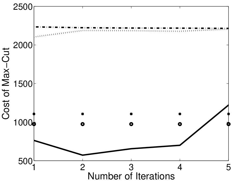
In this section, we show the results of our algorithm to solve max-cut on graphs with different configurations: trees, 2D-grid and random graphs. In all our experiments we restrict ourselves to , i.e., simple spanning trees. Given a set of weights in an undirected graph, , a cut is defined as . The function is known to be a non-monotone submodular function. To illustrate our algorithm, we generated synthetic graphs of different configurations with nodes and random positive edge weights. In the case of a tree-based cut functions, the algorithm converges to an optimal solution in the first iteration. In the case of 2D grid , the algorithm converges to an optimal solution as shown Figure 1-(a). We also show the performance of other constant factor approximation algorithm proposed by Buchbinder et al. [5] and Feige et al. [10] on this configuration. For generating random graphs, we considered nodes with random edge incident on each vertex with probability . It can be observed in Figure 1-(b) that our algorithm solves a convex optimization problem but with a larger integrality gap. This gap could be reduced by using higher treewidth graphs, i.e., instead of trees.
7 Conclusion
In this paper, we have developed a novel approximation framework for submodular functions, which enables us to provide convex relaxations of submodular function maximization and related problems. While we have considered only trees in our experiments, it is of clear interest to consider higher treewidths and explore empirically the trade-offs between computational complexity and tightness of our relaxations.
Acknowledgements
We acknowledge support from the European Research Council grant SIERRA (project 239993). We would also like to thank Nino Shervashidze for detailed feedback on the draft.
References
- [1] F. Bach. Learning with submodular functions: A convex optimization perspective. ArXiv e-prints, 2011.
- [2] D. P. Bertsekas and H. Yu. A unifying polyhedral approximation framework for convex optimization. SIAM Journal on Optimization, 21(1):333–360, 2011.
- [3] C. Bishop et al. Pattern recognition and machine learning. springer New York, 2006.
- [4] Y. Boykov, O. Veksler, and R. Zabih. Fast approximate energy minimization via graph cuts. IEEE Transactions on Pattern Analysis and Machine Intelligence (PAMI), 23(11):1222–1239, 2001.
- [5] N. Buchbinder, M. Feldman, N. Naor, Joseph, and R. Schwartz. A tight linear time (1/2)-approximation for unconstrained submodular maximization. In Proc. FOCS, 2012.
- [6] A. Chechetka and C. Guestrin. Efficient principled learning of thin junction trees. In Adv. NIPS, 2007.
- [7] D. M. Chickering. Optimal structure identification with greedy search. Journal of Machine Learning Research, 3:507–554, November 2002.
- [8] C. I. Chow and C. N. Liu. Approximating discrete probability distributions with dependence trees. IEEE Trans. Inf. Theory, 14, 1968.
- [9] T. M. Cover and J. A. Thomas. Elements of information theory. John Wiley & Sons, 2006.
- [10] U. Feige, V. S. Mirrokni, and J. Vondrák. Maximizing non-monotone submodular functions. SIAM J. Comput., 2011.
- [11] S. Fujishige. Submodular Functions and Optimization. Annals of Discrete Mathematics. Elsevier, 2005.
- [12] P. Giudici and P. Green. Decomposable graphical gaussian model determination. Biometrika, 86(4), 1999.
- [13] M. C. Golumbic. Algorithmic Graph Theory and Perfect Graphs. North Holland, 2004.
- [14] R. Iyer, S. Jegelka, and J. Bilmes. Fast semidifferential-based submodular function optimization. In Proc. ICML, pages 855–863, 2013.
- [15] D. Koller and N. Friedman. Probabilistic graphical models: principles and techniques. MIT press, 2009.
- [16] A. Krause and C. Guestrin. Near-optimal nonmyopic value of information in graphical models. In Proc. UAI, 2005.
- [17] A. Krause and C. Guestrin. Submodularity and its applications in optimized information gathering. ACM Transactions on Intelligent Systems and Technology, 2(4), 2011.
- [18] K. S. S. Kumar and F. Bach. Convex relaxations for learning bounded treewidth decomposable graphs. In Proc. ICML, 2013.
- [19] S. L. Lauritzen. Graphical Models. Oxford University Press, Oxford, 1996.
- [20] H. Lin and J. Bilmes. A class of submodular functions for document summarization. In Proc. NAACL/HLT, 2011.
- [21] K. P. Murphy. Machine learning: a probabilistic perspective. MIT Press, 2012.
- [22] M. Narasimhan and J. Bilmes. PAC-learning bounded tree-width graphical models. In Proc. UAI, 2004.
- [23] M. Narasimhan and J. Bilmes. A submodular-supermodular procedure with applications to discriminative structure learning. In Proc. UAI, 2005.
- [24] A. Nedic and A. Ozdaglar. Approximate primal solutions and rate analysis for dual subgradient methods. SIAM Journal on Optimization, 19(4):1757–1780, 2009.
- [25] G. Nemhauser, L. Wolsey, and M. Fisher. An analysis of approximations for maximizing submodular set functions–i. Mathematical Programming, 14(1):265–294, 1978.
- [26] H. D. Sherali and W. P. Adams. A hierarchy of relaxations between the continuous and convex hull representations for zero-one programming problems. SIAM J. Discrete Math., 1990.
- [27] D. Sontag, A. Globerson, and T. Jaakkola. Introduction to dual decomposition for inference. In Optimization for Machine Learning. MIT Press, 2011.
- [28] N. Srebro. Maximum likelihood bounded tree-width Markov networks. In Proc. UAI, 2002.
- [29] T. Szántai and E. Kovács. Hypergraphs as a mean of discovering the dependence structure of a discrete multivariate probability distribution. Annals OR, 193(1), 2012.
- [30] I. Tsochantaridis, T. Hofmann, T. Joachims, and Y. Altun. Support vector machine learning for interdependent and structured output spaces. In Proc. ICML, 2004.
- [31] J. Vondrák, C. Chekuri, and R. Zenklusen. Submodular function maximization via the multilinear relaxation and contention resolution schemes. In Proc. STOC, pages 783–792, 2011.
- [32] M. Wainwright, T. Jaakkola, and A. Willsky. A new class of upper bounds on the log partition function. IEEE Trans. Information Theory, 51(7), 2005.
- [33] M. Wainwright and M. Jordan. Treewidth-based conditions for exactness of the Sherali-Adams and Lasserre relaxations. Univ. California, Berkeley, Technical Report, 671, 2004.
- [34] M. Wainwright and M. Jordan. Graphical models, exponential families, and variational inference. Found. and Trends in Mach. Learn., 1(1-2), 2008.
- [35] A. L. Yuille and A. Rangarajan. The concave-convex procedure. Neural Computation, 2003.
- [36] Z. Zhang and R. W. Yeung. On characterization of entropy function via information inequalities. IEEE Trans. Inf. Theor., pages 1440–1452, 1998.
Appendix A Proof of Proposition 2
We have
where we have used acyclicity to ensure that for , .
Appendix B Proof of Proposition 3
Let and . If is a subgraph of , then and hence for all the vertices, , . Therefore, due to submodularity of ,
Appendix C Proof of Proposition 4
Assuming, without loss of generality, that is a topological ordering where , we have
since all terms are non-negative.
Appendix D Proof of Proposition 5
For a directed tree the bound is in fact a quadratic function of the indicator function , with quadratic terms equal to which are negative by submodularity of . The function is then a cut function and is submodular.
Appendix E Proof of Proposition 6
Two Markov equivalent graphs may be obtained by reversing orders of edges that are not involved in a “v-structure”. The result is then straightforward.
Appendix F Proof of Proposition 7
We first recall the two definitions.
| (6) |
| (7) |
Equivalence between Eq. (6) and Eq. (7) is a standard result in probabilistic graphical models, which states that if is a discrete distribution with strictly positive probability mass function that factorizes in , i.e.,
| (8) |
To show tightness of bounds on all cliques, we can always choose an elimination ordering where a given maximal clique is eliminated first, and we then obtain the tightness as a consequence of Prop. 2.
In order to show the monotonicity, notice that if is a subgraph of , then there is a sequence of decomposable graphs between and so that a single edge is added between two graphs in the sequence [12]. We can then show that at every forward step, the bound has to increase.
Finally, if a set is obtained by removing simplicial vertices of the graph, the relationship between DAGs and decomposable graphs and Prop. 4 leads to the desired result.
Appendix G Proof of Proposition 8
If for all cliques in , then for all and
which imples that .
In the context of probabilistic graphical models, this is equivalent to defining pseudo-marginals on the cliques and ensuring that the pseudo-marginals satisfy the local constraints of the marginal polytope. These are the order relaxations. The outer relaxation consists of all the extreme points of the marginal polytope as extreme points. However, it also consists of other additional extreme points with fractional elements. In the case of decomposable graph models, which are also known as hypertrees, these relaxations are shown to be tight and yield the same optimal solution [33, 34]. Therefore,
| (9) |
To prove the tightness, let us assume that there exists a decomposable graph, denoted by a vertex such that . Therefore,
| (10) | |||||