跳到论文正文
W Papers独立论文阅读器 arXiv:1309.2473 论文正文 计算阅读时间 · 0%
引用这篇论文根据当前论文元数据生成,正式投稿前建议核对。


License: arXiv.org perpetual non-exclusive license
arXiv:1309.2473v1 [cs.IT] 10 Sep 2013

Interference Alignment with Diversity for the 2×22\times 2 XX-Network with three antennas

Abhinav Ganesan and B. Sundar Rajan Affiliation: Email: {abhig_88, bsrajan}@ece.iisc.ernet.in
Abstract

Interference alignment is known to achieve the maximum sum DoF of 4​M3\frac{4M}{3} in the 2×22\times 2 XX-Network (i.e., two-transmitter (Tx) two-receiver (Rx) XX-Network) with MM antennas at each node, as demonstrated by Jafar and Shamai. Recently, an Alamouti code based transmission scheme, which we call the Li-Jafarkhani-Jafar (LJJ) scheme, was proposed for the 2×22\times 2 XX-Network with two antennas at each node. This scheme achieves a sum degrees of freedom (DoF) of 83\frac{8}{3} and also a diversity gain of two when fixed finite constellations are employed at each Tx. In the LJJ scheme, each Tx required the knowledge of only its own channel unlike the Jafar-Shamai scheme which required global CSIT to achieve the maximum possible sum DoF of 83\frac{8}{3}. Bit error rate (BER) is an important performance metric when the coding length is finite. This work first proposes a new STBC for a three transmit antenna single user MIMO system. Building on this STBC, we extend the LJJ scheme to the 2×22\times 2 XX-Network with three antennas at each node. Local channel knowledge is assumed at each Tx. It is shown that the proposed scheme achieves the maximum possible sum DoF of 44. A diversity gain of 33 is also guaranteed when fixed finite constellation inputs are used.

I Introduction

Maximizing the rate11 1 The definition of rate used here is in the sense of vanishing probability of error as given in Section 7.57.5 of [1]. of transmission and minimizing the bit error rate have been intensely pursued in single user communication systems. Multiple-input multiple-output (MIMO) systems offer the potential to improve both and hence, are immensely popular. Bit error rate is an issue in the case of coding over a fixed number of time slots while achievable rate is a performance metric when coding over infinite time slots is allowed. So, the design of space-time block codes (STBC) in single user MIMO systems incorporated two properties as performance metrics - the information losslessness property of an STBC and the diversity gain offered by an STBC [2, 3]. The former assures that the maximum achievable rate is not sacrificed by introduction of the STBC block in the MIMO system while the latter assures a degree of reliability in the data when the code length is restricted and SNR-independent finite constellation input is used.

Many recent works on multiuser communication systems, specifically on interference networks, have focused on sum-capacity optimal or approximate sum-capacity optimal transmission strategies. The notion of approximate sum-capacity is captured by the concept of degrees of freedom (DoF). The sum DoF of a Gaussian interference network is said to be dd if the sum-capacity can be written as d​l​o​g2​S​N​R+o⁡(l​o​g2​S​N​R)d~log_{2}SNR+o(log_{2}SNR) [4]. Wireless XX-Networks are a class of Gaussian interference networks with KK transmitters and JJ receivers where every receiver demands an independent message from every transmitter so that there is a total of K​JKJ messages meant to be transmitted in the network. We shall denote an XX network with MM antennas at every node by (K,J,M)−X(K,J,M)-X-Network. A sum DoF of ⌊4​M3⌋\lfloor{\frac{4M}{3}}\rfloor was shown to be achievable in a (2,2,M)−X(2,2,M)-X-Network in [5] while Jafar and Shamai in [4] showed that a sum DoF of 4​M3\frac{4M}{3} is achievable using the idea of interference alignment (IA)22 2 We shall henceforth call the transmission scheme proposed in [4] as the JS scheme.. Further, 4​M3\frac{4M}{3} is proven [4] to be an outerbound on the sum DoF of (2,2,M)−X(2,2,M)-X-Network which establishes 4​M3\frac{4M}{3} to be the sum DoF of (2,2,M)−X(2,2,M)-X-Network.

Recently, Alamouti codes were intelligently coupled with channel dependent precoding [6, 7] to achieve a sum-DoF of 83\frac{8}{3} in the (2,2,2)−X(2,2,2)-X-Network. Also, a diversity gain of two was assured. The transmission scheme in [6] shall be referred to as the LJJ scheme. In a sense, the performance metrics that the LJJ scheme highlights i.e., achieving the maximum sum DoF and a diversity gain that is strictly greater than one, is akin to the properties sought after in the design of STBCs for single user communication systems i.e., the information losslessness property and the diversity gain. Note that sum DoF is an approximate sum-capacity at high SNR. Thus, STBCs with information losslessness property that were sought after in single user systems is now translated to approximate sum-capacity lossless design of STBCs in the (2,2,2)−X(2,2,2)-X-Network. The design of STBCs that offer diversity gain in (2,2,M)−X(2,2,M)-X-Network however comes with a crucial difference with respect to the single user scenario. Local channel knowledge (i.e., every transmitter knows only its own channel) is assumed in the LJJ scheme for the (2,2,2)−X(2,2,2)-X-Network whereas the design of information lossless STBCs in the single user set-up does not assume CSIT. Similarly, an extension of the LJJ scheme for the (2,2,4)−X(2,2,4)-X-Network [8] using the Srinath-Rajan (SR) STBC [9] assumed local channel knowledge. Assumption of no CSIT would make things difficult. Even the JS scheme assumed global CSIT, i.e., knowledge of all the channel gains at all the transmitters, to achieve sum DoF of 4​M3\frac{4M}{3}.

The challenge in extending the LJJ scheme to a general (2,2,M)−X(2,2,M)-X-Network is to identify STBCs that could be applied in the (2,2,M)−X(2,2,M)-X-Network with appropriate modifications. This was done for M=4M=4 in [8] where the SR STBC fitted nicely into the extended LJJ scheme. This work aims to extend the LJJ scheme to the (2,2,3)−X(2,2,3)-X-Network. As in the LJJ scheme and the extended LJJ scheme for the (2,2,4)−X(2,2,4)-X-Network using the SR STBC, the performance metrics are the achievable sum DoF and the diversity gain. The contributions of this work are summarized below.

  • •

    We propose an STBC that encodes 32\frac{3}{2} complex symbols per channel use (cspcu) for a three transmit antenna single user MIMO system. We use this STBC in the extended LJJ scheme to achieve the maximum sum DoF of 44 in the (2,2,3)−X(2,2,3)-X-Network (Theorem 2, Section IV). Like the LJJ scheme, the proposed scheme assumes only local channel knowledge at the transmitters.

  • •

    We show that the proposed scheme guarantees a diversity gain of 33 when fixed finite constellation inputs are used (Theorem 1, Section IV). Simulation results show that the diversity gain is strictly greater than 33.

The paper is organized as follows. The next section formally introduces the system model. Section III summarizes the JS scheme and the LJJ scheme. The proposed scheme is explained in Section IV where the DoF achievability and the diversity gain achieved are also proved. Section V presents simulation results illustrating the performance of the proposed scheme. The paper concludes with Section VI.

Notations: The set of complex numbers is denoted by ℂ\mathbb{C}. The notation 𝒞𝒩⁡(0,σ2){\cal CN}(0,\sigma^{2}) denotes the circularly symmetric complex Gaussian distribution with mean zero and variance σ2\sigma^{2}. For a complex number xx, the notation x¯\overline{x} denotes the conjugate of xx. The real and imaginary parts of a complex number aa are denoted by aRa^{R} and aIa^{I} respectively. The identity matrix of size n×nn\times n is denoted by InI_{n}. An all-zeros column vector is denoted by 0¯\underline{0}. The trace of a matrix AA is denoted by tr​(A)\text{tr}(A). For an invertible matrix AA, the notation A−HA^{-H} denotes the Hermitian of the matrix A−1A^{-1}. The ithi^{\text{th}} row and the ithi^{\text{th}} column of a matrix AA are denoted by A(i,:)A(i,:) and A(:,i)A(:,i) respectively. The ithi^{\text{th}} row, jthj^{\text{th}} column element of a matrix AA is denoted by A⁡(i,j)A(i,j) unless mentioned otherwise. The Frobenius norm of a matrix AA is denoted by ‖A‖||A||. The Kronecker product of two matrices AA and BB is denoted by A⊗BA\otimes B. A diagonal matrix with the diagonal entries given by a1,a2,⋯,ana_{1},a_{2},\cdots,a_{n} is denoted by diag​(a1,a2,⋯,an)\text{diag}(a_{1},a_{2},\cdots,a_{n}).

II System Model

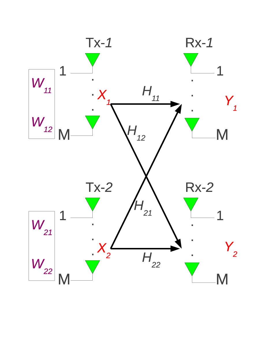
The (2,2,M)−X(2,2,M)-X-Network is shown in Fig. 1. The message transmitted by transmitter (Tx) ii to receiver (Rx) jj is represented by Wi​jW_{ij}.

Refer to caption
Fig. 1: System Model.

The input-output relation over TT time slots is given by

Yj=P​∑i=12Hi​j​Xi+Nj\displaystyle Y_{j}=\sqrt{P}\sum_{i=1}^{2}H_{ij}X_{i}+N_{j} (1)

where, Yj∈ℂM×TY_{j}\in\mathbb{C}^{M\times T} denotes the output symbol matrix at Rx-jj, Xi∈ℂM×TX_{i}\in\mathbb{C}^{M\times T} denotes the input symbol matrix at Tx-ii such that 𝔼⁡[tr​(X​XH)]≤T\mathbb{E}\left[\text{tr}\left(XX^{H}\right)\right]\leq T, Hi​j∈ℂM×MH_{ij}\in\mathbb{C}^{M\times M} denotes the channel matrix between Tx-ii and Rx-jj, Nj∈ℂM×TN_{j}\in\mathbb{C}^{M\times T} denotes the noise matrix whose entries are distributed as i.i.d. 𝒞𝒩⁡(0,1){\cal CN}(0,1). The average power constraint at each of the transmitters is denoted by PP. The channel gains are assumed to be constant for the length of the codeword, and the real and imaginary parts of the channel gains are distributed independently according to an arbitrary continuous distribution. Global CSIR is assumed throughout the paper, i.e., both the receivers have the knowledge of all the channel gains.

III Review of some known transmission schemes in (2,2,M)−X(2,2,M)-X-Network

In the first sub-section, the JS scheme is reviewed and in the second sub-section, the LJJ scheme for the (2,2,2)−X(2,2,2)-X-Network is reviewed.

III-A Review of JS Scheme for (2,2,3)−X(2,2,3)-X-Network

The JS scheme for (2,2,3)−X(2,2,3)-X-Network aligns the interference symbols by precoding over a 33-symbol extension of the channel, i.e., T=3T=3. Every transmitter sends 33 complex symbols to each receiver over 33 channel uses so that a sum DoF of 44 is attained. The input and the output symbols over a 33-symbol extension of the channel are related by

Yj′=3​P2​∑i=12Hi​j′​(∑k=12Vi​ktr​(Vi​k​Vi​kH)​Xi​k)+Nj′\displaystyle Y^{\prime}_{j}=\sqrt{\frac{3P}{2}}\sum_{i=1}^{2}H^{\prime}_{ij}\left(\sum_{k=1}^{2}\frac{V_{ik}}{\text{tr}\left(V_{ik}V^{H}_{ik}\right)}X_{ik}\right)+N^{\prime}_{j} (2)

where, Yj′∈ℂ9×1Y^{\prime}_{j}\in\mathbb{C}^{9\times 1} denotes the received symbol vector at Rx-jj over 33 channel uses, Hi​j′=[Hi​j𝟎𝟎𝟎Hi​j𝟎𝟎𝟎Hi​j]H^{\prime}_{ij}=\begin{bmatrix}H_{ij}&\mathbf{0}&\mathbf{0}\\ \mathbf{0}&H_{ij}&\mathbf{0}\\ \mathbf{0}&\mathbf{0}&H_{ij}\end{bmatrix} denotes the effective channel matrix between Tx-ii and Rx-jj over 33 channel uses, Vi​k∈ℂ9×3V_{ik}\in\mathbb{C}^{9\times 3} denotes a precoding matrix, Xi​k∈ℂ3×1X_{ik}\in\mathbb{C}^{3\times 1} denotes the symbol vector generated by Tx-ii meant for Rx-kk, and Nj′∈ℂ9×1N^{\prime}_{j}\in\mathbb{C}^{9\times 1} denotes the Gaussian noise vector whose entries are distributed as i.i.d. 𝒞𝒩⁡(0,1){\cal CN}(0,1). The entries of Xi​kX_{ik} take values from a set such that 𝔼⁡[Xi​k​Xi​kH]=I3\mathbb{E}\left[X_{ik}X^{H}_{ik}\right]=I_{3}. The precoders Vi​kV_{ik} are chosen as given below.

V11=EF′​V1F′,V12=EF′​V2F′,\displaystyle V_{11}=E^{F^{\prime}}{V^{F^{\prime}}_{1}},~~V_{12}=E^{F^{\prime}}{V^{F^{\prime}}_{2}},
V21=H′22−1​H12′​V11,V22=H′21−1​H11′​V12\displaystyle V_{21}={H^{\prime}}^{-1}_{22}H^{\prime}_{12}V_{11},~~~V_{22}={H^{\prime}}^{-1}_{21}H^{\prime}_{11}V_{12}

where, EF′∈ℂ9×9E^{F^{\prime}}\in\mathbb{C}^{9\times 9} denotes a matrix whose columns are the eigen vectors of the matrix F′=H′11−1​H21′​H′22−1​H12′F^{\prime}={H^{\prime}}^{-1}_{11}H^{\prime}_{21}{H^{\prime}}^{-1}_{22}H^{\prime}_{12}, V1F′=I3⊗[1​1​0]TV^{F^{\prime}}_{1}=I_{3}\otimes[1~1~0]^{T}, and V2F′=I3⊗[1​0​1]TV^{F^{\prime}}_{2}=I_{3}\otimes[1~0~1]^{T}. Using the above choice of precoders, the interference symbols are aligned and (2) can be re-written as

Y1′=3​P2​(H11′​V11​X11+H21′​V21​X21CLOSE\displaystyle Y^{\prime}_{1}=\sqrt{\frac{3P}{2}}\left(H^{\prime}_{11}V_{11}X_{11}+H^{\prime}_{21}V_{21}X_{21}\right.
OPEN+H11​V12​(X12+X22))+N1′\displaystyle\hskip 113.81102pt\left.+H_{11}V_{12}\left(X_{12}+X_{22}\right)\right)+N^{\prime}_{1}
Y2′=3​P2​(H12′​V12​X12+H22′​V22​X22CLOSE\displaystyle Y^{\prime}_{2}=\sqrt{\frac{3P}{2}}\left(H^{\prime}_{12}V_{12}X_{12}+H^{\prime}_{22}V_{22}X_{22}\right. (3)
OPEN+H12​V11​(X11+X21))+N2′.\displaystyle\hskip 113.81102pt\left.+H_{12}V_{11}\left(X_{11}+X_{21}\right)\right)+N^{\prime}_{2}.

The above described scheme is proved to achieve a sum DoF of 44 in the (2,2,3)−X(2,2,3)-X-Network almost surely when the channel matrix entries take values from a continuous probability distribution [4].

III-B Review of LJJ Scheme

The LJJ scheme for the (2,2,2)−X(2,2,2)-X-Network transmits two superposed Alamouti codes with appropriate precoding in three time slots (i.e., T=3T=3) at every transmitter. The symbols meant for each receiver are transmitted through an Alamouti code as given by

X1\displaystyle X_{1} =3​P4​(V11​[x111−x112¯0x112x111¯0]⏟X11+V12​[0x121−x122¯0x122x121¯]⏟X12)\displaystyle=\sqrt{\frac{3P}{4}}\left(V_{11}\underbrace{\begin{bmatrix}x^{1}_{11}&-\overline{x^{2}_{11}}&0\\ x^{2}_{11}&~\overline{x^{1}_{11}}&0\end{bmatrix}}_{X_{11}}+V_{12}\underbrace{\begin{bmatrix}0&x^{1}_{12}&-\overline{x^{2}_{12}}\\ 0&x^{2}_{12}&~\overline{x^{1}_{12}}\end{bmatrix}}_{X_{12}}\right)
X2\displaystyle X_{2} =3​P4​(V22​[x211−x212¯0x212x211¯0]⏟X21+V12​[0x221−x222¯0x222x221¯]⏟X22)\displaystyle=\sqrt{\frac{3P}{4}}\left(V_{22}\underbrace{\begin{bmatrix}x^{1}_{21}&-\overline{x^{2}_{21}}&0\\ x^{2}_{21}&~\overline{x^{1}_{21}}&0\end{bmatrix}}_{X_{21}}+V_{12}\underbrace{\begin{bmatrix}0&x^{1}_{22}&-\overline{x^{2}_{22}}\\ 0&x^{2}_{22}&~\overline{x^{1}_{22}}\end{bmatrix}}_{X_{22}}\right)

where, xi​jkx^{k}_{ij} takes values from a set such that 𝔼⁡[|xi​jk|2]=1\mathbb{E}\left[\left|x^{k}_{ij}\right|^{2}\right]=1. The matrices Xi​jX_{ij}, as defined above, correspond to the symbols generated by Tx-ii meant for Rx-jj. The matrix entries xi​jkx^{k}_{ij} denote the kthk^{\text{th}} symbol generated by Tx-ii for Rx-jj. The precoders Vi​jV_{ij} are chosen as

V11=H12−1tr​(H12−1​H12−H),V12=H11−1tr​(H11−1​H11−H)\displaystyle V_{11}=\frac{H^{-1}_{12}}{\sqrt{\text{tr}\left(H^{-1}_{12}H^{-H}_{12}\right)}},~V_{12}=\frac{H^{-1}_{11}}{\sqrt{\text{tr}\left(H^{-1}_{11}H^{-H}_{11}\right)}}
V21=H22−1tr​(H22−1​H22−H),V22=H21−1tr​(H21−1​H21−H).\displaystyle V_{21}=\frac{H^{-1}_{22}}{\sqrt{\text{tr}\left(H^{-1}_{22}H^{-H}_{22}\right)}},~V_{22}=\frac{H^{-1}_{21}}{\sqrt{\text{tr}\left(H^{-1}_{21}H^{-H}_{21}\right)}}. (4)

The terms inside the square-roots above ensure that the transmitters meet the average power constraint. We briefly describe how the above choice of precoders and the use of Alamouti codes whose columns are juxtaposed with a zero column help to align the interference. The output symbol matrix at Rx-11 is now given by

Y1=3​P4​H11​V11​X11+3​P4​H21​V21​X21\displaystyle Y_{1}=\sqrt{\frac{3P}{4}}H_{11}V_{11}X_{11}+\sqrt{\frac{3P}{4}}H_{21}V_{21}X_{21}
+3​P4​[0a​x121+b​x221−a​x122¯−b​x222¯0a​x122+b​x222a​x121¯+b​x221¯]+N1\displaystyle~~~~~~~~+\sqrt{\frac{3P}{4}}\begin{bmatrix}0&ax^{1}_{12}+bx^{1}_{22}&-a\overline{x^{2}_{12}}-b\overline{x^{2}_{22}}\\ 0&ax^{2}_{12}+bx^{2}_{22}&~a\overline{x^{1}_{12}}+b\overline{x^{1}_{22}}\end{bmatrix}+N_{1}

where, a=1tr​(H11−1​H11−H)a=\frac{1}{\sqrt{\text{tr}\left(H^{-1}_{11}H^{-H}_{11}\right)}} and b=1tr​(H21−1​H21−H)b=\frac{1}{\sqrt{\text{tr}\left(H^{-1}_{21}H^{-H}_{21}\right)}}. Let the effective channel matrices corresponding to the desired symbols from Tx-11 and Tx-22 to Rx-11 be denoted by H^=H11​V11\hat{H}=H_{11}V_{11} and G^=H21​V21\hat{G}=H_{21}V_{21} respectively. Define a matrix Y′∈ℂ2×3Y^{\prime}\in\mathbb{C}^{2\times 3} whose first, second and third columns are given by

Y′(:,1)=Y(:,1),Y′(:,2)=Y(:,1)¯,Y′(:,3)=Y(:,3).\displaystyle Y^{\prime}(:,1)=Y(:,1),~Y^{\prime}(:,2)=\overline{Y(:,1)},~Y^{\prime}(:,3)=Y(:,3). (5)

Similarly, define the matrix N1′N^{\prime}_{1} obtained from N1N_{1}. The processed output symbols at Rx-11 (i.e., Y1′Y^{\prime}_{1}) can be written as

[Y′1T(1,:)Y′1T(2,:)]⏟Y1′′=3​P4\displaystyle\underbrace{\begin{bmatrix}{Y^{\prime}}_{1}^{T}(1,:)\\ {Y^{\prime}}_{1}^{T}(2,:)\end{bmatrix}}_{Y^{\prime\prime}_{1}}=\sqrt{\frac{3P}{4}} [h^11h^12g^11g^1200h^12¯−h^11¯g^12¯−h^11¯1000000−1h^21h^22g^21g^2200h^22¯−h^21¯g^22¯−h^21¯01000010]​[x111x112x211x212I1I2]\displaystyle\begin{bmatrix}\hat{h}_{11}&\hat{h}_{12}&\hat{g}_{11}&\hat{g}_{12}&0&0\\ \overline{\hat{h}_{12}}&-\overline{\hat{h}_{11}}&\overline{\hat{g}_{12}}&-\overline{\hat{h}_{11}}&1&0\\ 0&0&0&0&0&-1\\ \hat{h}_{21}&\hat{h}_{22}&\hat{g}_{21}&\hat{g}_{22}&0&0\\ \overline{\hat{h}_{22}}&-\overline{\hat{h}_{21}}&\overline{\hat{g}_{22}}&-\overline{\hat{h}_{21}}&0&1\\ 0&0&0&0&1&0\end{bmatrix}\begin{bmatrix}x^{1}_{11}\\ x^{2}_{11}\\ x^{1}_{21}\\ x^{2}_{21}\\ I_{1}\\ I_{2}\end{bmatrix}
+[N′1T(1,:)N′1T(2,:)]⏟N1′′\displaystyle\hskip 28.45274pt+\underbrace{\begin{bmatrix}{N^{\prime}}_{1}^{T}(1,:)\\ {N^{\prime}}_{1}^{T}(2,:)\end{bmatrix}}_{N^{\prime\prime}_{1}} (6)

where, I1=a​x121¯+b​x221¯I_{1}=a\overline{x^{1}_{12}}+b\overline{x^{1}_{22}} and I2=a​x122¯+b​x222¯I_{2}=a\overline{x^{2}_{12}}+b\overline{x^{2}_{22}}, and h^i​j\hat{h}_{ij} and g^i​j\hat{g}_{ij} denote the entries of the matrices H^\hat{H} and G^\hat{G} respectively. Note that, when h^i​j\hat{h}_{ij} and g^i​j\hat{g}_{ij} are non-zero, the interference symbols I1I_{1} and I2I_{2} are aligned in a subspace linearly independent of the signal subspace. So, pre-multiplying the matrix Y1′′Y^{\prime\prime}_{1} (defined in (6)) by the zero-forcing matrix given by

F=[10000001000−1001010000100]\displaystyle F=\begin{bmatrix}1&0&0&0&0&0\\ 0&1&0&0&0&-1\\ 0&0&1&0&1&0\\ 0&0&0&1&0&0\end{bmatrix} (7)

yields

F​Y1′′=3​P4​[h^11h^12g^11g^12h^12¯−h^11¯g^12¯−h^11¯h^21h^22g^21g^22h^22¯−h^21¯g^22¯−h^21¯]⏟R​[x111x112x211x212]+F​N1′′.\displaystyle FY^{\prime\prime}_{1}=\sqrt{\frac{3P}{4}}\underbrace{\begin{bmatrix}\hat{h}_{11}&\hat{h}_{12}&\hat{g}_{11}&\hat{g}_{12}\\ \overline{\hat{h}_{12}}&-\overline{\hat{h}_{11}}&\overline{\hat{g}_{12}}&-\overline{\hat{h}_{11}}\\ \hat{h}_{21}&\hat{h}_{22}&\hat{g}_{21}&\hat{g}_{22}\\ \overline{\hat{h}_{22}}&-\overline{\hat{h}_{21}}&\overline{\hat{g}_{22}}&-\overline{\hat{h}_{21}}\\ \end{bmatrix}}_{R}\begin{bmatrix}x^{1}_{11}\\ x^{2}_{11}\\ x^{1}_{21}\\ x^{2}_{21}\\ \end{bmatrix}+FN^{\prime\prime}_{1}. (8)

It is shown that the matrix RR is almost surely full rank and hence, a sum DoF of 83\frac{8}{3} is achieved in the (2,2,2)−X(2,2,2)-X-Network. When the symbols xi​jkx^{k}_{ij} take values from finite constellations, it is proved that a diversity gain of 22 can be achieved for every xi​jkx^{k}_{ij}, along with symbol-by-symbol decoding [7].

The LJJ scheme is extended to the (2,2,3)−X(2,2,3)-X-Network in the next section.

IV Extended LJJ scheme for the (2,2,3)−X(2,2,3)-X-Network

In this section, we first present a set of conditions on STBCs, which when coupled with LJJ-type precoding, could be used in a general (2,2,M)−X(2,2,M)-X-Network to achieve a diversity gain of MM. We then present an explicit construction of an STBC for the (2,2,3)−X(2,2,3)-X-Network which achieves a diversity gain of 33 and a sum DoF of 44 with Gaussian input alphabets. Throughout this section, we shall focus only on decoding the desired symbols and interference cancellation at Rx-11. Similar signal processing is assumed to happen at Rx-22.

Consider a M×T′M\times T^{\prime} linear dispersion STBC denoted by X′X^{\prime} where T′≥MT^{\prime}\geq M is an even integer. Linear dispersion STBCs are those which can be represented as X′=∑i=1LAi​R​xi​R+Ai​I​xi​IX^{\prime}=\sum_{i=1}^{L}A^{iR}x^{iR}+A^{iI}x^{iI} where, xi∈𝒮x^{i}\in{\cal S} represent the symbols that the STBC encodes for some finite constellation 𝒮{\cal S}, and the matrices Ai​R,Ai​I∈ℂM×T′A^{iR},A^{iI}\in\mathbb{C}^{M\times T^{\prime}} are called dispersion matrices [10]. Every transmitter uses an STBC with the same structure as that of X′X^{\prime} to transmit its message symbols to each of the receivers. Let the STBC corresponding to the symbols meant to be sent from Tx-ii to Rx-jj be denoted by Xi​j′X^{\prime}_{ij}, i,j=1,2i,j=1,2. Consider a matrix Xi​1X_{i1} formed by inserting a zero column to every third column of Xi​1′X^{\prime}_{i1} so that there are a total of T′2\frac{T^{\prime}}{2} all-zero columns, i.e., a column of zeros is inserted after every two columns of Xi​1′X^{\prime}_{i1}, starting from its third column. Also, consider a matrix Xi​2X_{i2} formed by inserting a zero column to every third column of Xi​2′X^{\prime}_{i2}, but starting from its first column (i.e., the first column of Xi​2X_{i2} is an all-zero column), so that there are a total of T′2\frac{T^{\prime}}{2} all-zero columns. Note that the matrices Xi​jX_{ij} are M×3​T′2M\times\frac{3T^{\prime}}{2} matrices. The precoders used are the same as in the LJJ scheme, i.e., given by (4). The received symbols at Rx-11 are given by

Y1\displaystyle Y_{1} =c1​P​H11​V11​X11+c2​P​H21​V21​X21\displaystyle=\sqrt{c_{1}P}H_{11}V_{11}X_{11}+\sqrt{c_{2}P}H_{21}V_{21}X_{21}
+c1​P​a​X12+c2​P​b​X22+N1\displaystyle+\sqrt{c_{1}P}aX_{12}+\sqrt{c_{2}P}bX_{22}+N_{1}

where, cic_{i} is a normalizing constant which ensures that the power constraint at Tx-ii is met. Note that the received symbols at time instants t=1,4,7,⋯,3​T′2−2t=1,4,7,\cdots,\frac{3T^{\prime}}{2}-2 are interference-free because of the pattern of the zero columns in Xi​2X_{i2}. The unintended symbols interfere at time instants t=2,5,8,⋯,3​T′2−1t=2,5,8,\cdots,\frac{3T^{\prime}}{2}-1, at Rx-11. We now narrow down on a desirable structure of the STBC X′X^{\prime} so that the interfering symbols can be canceled. Let fk:ℂ→ℂf_{k}:\mathbb{C}\rightarrow\mathbb{C} be a deterministic function such that fk​(w)f_{k}(w) is distributed as 𝒞𝒩⁡(0,σk2){\cal CN}(0,\sigma_{k}^{2}) when ww is distributed as 𝒞𝒩⁡(0,1){\cal CN}(0,1), for k=1,2,⋯,M​T′2k=1,2,\cdots,\frac{MT^{\prime}}{2}. Let πp\pi_{p} be a permutation of {1,2,⋯,M}\{1,2,\cdots,M\}, for p=1,3,⋯,T′−1p=1,3,\cdots,T^{\prime}-1. Suppose there exist functions fkf_{k} such that

X′(:,p)+[f(p−1)​M2+1​(X′​(πp​(1),p+1))f(p−1)​M2+2​(X′​(πp​(2),p+1))f(p−1)​M2+M​(X′​(πp​(M),p+1))]=0¯\displaystyle X^{\prime}(:,p)+\begin{bmatrix}f_{\frac{(p-1)M}{2}+1}(X^{\prime}(\pi_{p}(1),p+1))\\ f_{\frac{(p-1)M}{2}+2}(X^{\prime}(\pi_{p}(2),p+1))\\ \vdots\\ f_{\frac{(p-1)M}{2}+M}(X^{\prime}(\pi_{p}(M),p+1))\\ \end{bmatrix}=\underline{0}

for p=1,3,⋯,T′−1p=1,3,\cdots,T^{\prime}-1. We call the above property of the STBC X′X^{\prime} as the column cancellation property.

We observe that the signal corresponding to the desired symbols is equal to zero at time instants t=3,6,9,⋯,3​T′2t=3,6,9,\cdots,\frac{3T^{\prime}}{2}, at Rx-11 because of the pattern of zero-columns in Xi​1X_{i1}, for i=1,2i=1,2. Thus, on the account of the column cancellation property of X′X^{\prime} clearly, the interference symbols at time instants t=2,5,8,⋯,3​T′2−1t=2,5,8,\cdots,\frac{3T^{\prime}}{2}-1 can be canceled using the interference symbols received at time instants t=3,6,9,⋯,3​T′2t=3,6,9,\cdots,\frac{3T^{\prime}}{2}, without affecting the desired symbols at Rx-11. Now, the relevant components of the noise vectors corresponding to the time instants t=2,5,8,⋯,3​T′2−1t=2,5,8,\cdots,\frac{3T^{\prime}}{2}-1, are distributed as i.i.d. 𝒞𝒩⁡(0,1+σk2){\cal CN}(0,1+\sigma_{k}^{2}), for k=1,2,⋯M​T′2k=1,2,\cdots\frac{MT^{\prime}}{2}. Discarding the received symbols at time instants t=3,6,9,⋯,3​T′2t=3,6,9,\cdots,\frac{3T^{\prime}}{2}, the processed received symbols at Rx-11 which are now interference-free can be written as

Y1′=c1​P​H11​V11​X11′+c2​P​H21​V21​X21′+N1′\displaystyle Y^{\prime}_{1}=\sqrt{c_{1}P}H_{11}V_{11}X^{\prime}_{11}+\sqrt{c_{2}P}H_{21}V_{21}X^{\prime}_{21}+N^{\prime}_{1} (9)

where, Xi​j′X^{\prime}_{ij} is obtained from Xi​jX_{ij} by dropping the all-zero columns. The following theorem states the condition on X′X^{\prime} under which ML decoding of Xi​1′X^{\prime}_{i1} from (9) yields a diversity gain of MM.

Define the difference matrix △​Xi​j′k1,k2\triangle{X^{\prime k_{1},k_{2}}_{ij}} by

△​Xi​j′k1,k2=Xi​j′k1−Xi​j′k2\displaystyle\triangle{X^{\prime k_{1},k_{2}}_{ij}}={X^{\prime k_{1}}_{ij}}-{X^{\prime k_{2}}_{ij}}

where, Xi​j′k1{X^{\prime k_{1}}_{ij}} and Xi​j′k2{X^{\prime k_{2}}_{ij}} denote two different realizations (i.e., k1≠k2k_{1}\neq k_{2}) of the matrix Xi​j′X^{\prime}_{ij}. We note that the finite constellations involved with the STBCs Xi​j′X^{\prime}_{ij} for different (i,j)(i,j) could be different.

Theorem 1

If the channel matrix entries are distributed as i.i.d. 𝒞𝒩⁡(0,1){\cal CN}(0,1) then, the average pair-wise error probability PeP_{e} for the distinct pairs of codewords (X11′k1,X21′k2)\left({X^{\prime k_{1}}_{11}},{X^{\prime k_{2}}_{21}}\right) and (X11′k1′,X21′k2′)\left({X^{\prime k^{\prime}_{1}}_{11}},{X^{\prime k^{\prime}_{2}}_{21}}\right) is upper bounded as

Pe​((X11′k1,X21′k2)→(X11′k1′,X21′k2′))≤c​P−M\displaystyle P_{e}\left({\left({X^{\prime k_{1}}_{11}},{X^{\prime k_{2}}_{21}}\right)\rightarrow\left({X^{\prime k^{\prime}_{1}}_{11}},{X^{\prime k^{\prime}_{2}}_{21}}\right)}\right)\leq cP^{-M}

for some constant c>0c>0, when the difference matrices △​Xi​1′k1,k2\triangle{X^{\prime k_{1},k_{2}}_{i1}} are full rank for all k1≠k2k_{1}\neq k_{2} and for i=1,2i=1,2.

Proof:

The proof is a generalization of the proof of Theorem 44 in [8]. The proof is given in Appendix A. ∎

An STBC X′X^{\prime} for M=3M=3 which possesses the column cancellation property is given in (10).

X′=[x1​R+j​x3​I−x2​R+j​x4​Iej​θ​(x5​R+j​x6​I)ej​θ​(−x3​R+j​x1​I)x2​R+j​x4​Ix1​R−j​x3​Iej​θ​(x4​R+j​x2​I)ej​θ​(x5​R−j​x6​I)ej​θ​(x6​R+j​x5​I)ej​θ​(−x6​R+j​x5​I)x3​R+j​x1​I−x4​R+j​x2​I]\displaystyle X^{\prime}=\begin{bmatrix}x^{1R}+jx^{3I}&-x^{2R}+jx^{4I}&e^{j\theta}\left(x^{5R}+jx^{6I}\right)&e^{j\theta}\left(-x^{3R}+jx^{1I}\right)\\ x^{2R}+jx^{4I}&x^{1R}-jx^{3I}&e^{j\theta}\left(x^{4R}+jx^{2I}\right)&e^{j\theta}\left(x^{5R}-jx^{6I}\right)\\ e^{j\theta}\left(x^{6R}+jx^{5I}\right)&e^{j\theta}\left(-x^{6R}+jx^{5I}\right)&x^{3R}+jx^{1I}&-x^{4R}+jx^{2I}\\ \end{bmatrix} (10)


The matrices Xi​1X_{i1} and Xi​2X_{i2} in the (2,2,3)−X(2,2,3)-X-Network are given by (11) and (12) respectively. It is assumed that the symbols xi​jkx^{k}_{ij} take values from a finite constellation 𝒮i​j{\cal S}_{ij} whose average energy is equal to one. The constants c1c_{1} and c2c_{2} are given by c1=c2=34c_{1}=c_{2}=\frac{3}{4}.

Xi​1=[xi​11​R+j​xi​13​I−xi​12​R+j​xi​14​I0ej​θ​(xi​15​R+j​xi​16​I)ej​θ​(−xi​13​R+j​xi​11​I)0xi​12​R+j​xi​14​Ixi​11​R−j​xi​13​I0ej​θ​(xi​14​R+j​xi​12​I)ej​θ​(xi​15​R−j​xi​16​I)0ej​θ​(xi​16​R+j​xi​15​I)ej​θ​(−xi​16​R+j​xi​15​I)0xi​13​R+j​xi​11​I−xi​14​R+j​xi​12​I0]\displaystyle X_{i1}=\begin{bmatrix}x^{1R}_{i1}+jx^{3I}_{i1}&-x^{2R}_{i1}+jx^{4I}_{i1}&0&e^{j\theta}\left(x^{5R}_{i1}+jx^{6I}_{i1}\right)&e^{j\theta}\left(-x^{3R}_{i1}+jx^{1I}_{i1}\right)&0\\ x^{2R}_{i1}+jx^{4I}_{i1}&x^{1R}_{i1}-jx^{3I}_{i1}&0&e^{j\theta}\left(x^{4R}_{i1}+jx^{2I}_{i1}\right)&e^{j\theta}\left(x^{5R}_{i1}-jx^{6I}_{i1}\right)&0\\ e^{j\theta}\left(x^{6R}_{i1}+jx^{5I}_{i1}\right)&e^{j\theta}\left(-x^{6R}_{i1}+jx^{5I}_{i1}\right)&0&x^{3R}_{i1}+jx^{1I}_{i1}&-x^{4R}_{i1}+jx^{2I}_{i1}&0\\ \end{bmatrix} (11)

 
Xi​2=[0xi​21​R+j​xi​23​I−xi​22​R+j​xi​24​I0ej​θ​(xi​25​R+j​xi​26​I)ej​θ​(−xi​23​R+j​xi​21​I)0xi​22​R+j​xi​24​Ixi​21​R−j​xi​23​I0ej​θ​(xi​24​R+j​xi​22​I)ej​θ​(xi​25​R−j​xi​26​I)0ej​θ​(xi​26​R+j​xi​25​I)ej​θ​(−xi​26​R+j​xi​25​I)0xi​23​R+j​xi​21​I−xi​24​R+j​xi​22​I]\displaystyle X_{i2}=\begin{bmatrix}0&x^{1R}_{i2}+jx^{3I}_{i2}&-x^{2R}_{i2}+jx^{4I}_{i2}&0&e^{j\theta}\left(x^{5R}_{i2}+jx^{6I}_{i2}\right)&e^{j\theta}\left(-x^{3R}_{i2}+jx^{1I}_{i2}\right)\\ 0&x^{2R}_{i2}+jx^{4I}_{i2}&x^{1R}_{i2}-jx^{3I}_{i2}&0&e^{j\theta}\left(x^{4R}_{i2}+jx^{2I}_{i2}\right)&e^{j\theta}\left(x^{5R}_{i2}-jx^{6I}_{i2}\right)\\ 0&e^{j\theta}\left(x^{6R}_{i2}+jx^{5I}_{i2}\right)&e^{j\theta}\left(-x^{6R}_{i2}+jx^{5I}_{i2}\right)&0&x^{3R}_{i2}+jx^{1I}_{i2}&-x^{4R}_{i2}+jx^{2I}_{i2}\\ \end{bmatrix} (12)


The interference cancellation at Rx-11 is done as follows. The matrix Y1′∈ℂ3×4Y^{\prime}_{1}\in\mathbb{C}^{3\times 4} obtained by processing Y1∈ℂ3×6Y_{1}\in\mathbb{C}^{3\times 6} is given below.

Y1′(:,1)=Y1(:,1),\displaystyle Y^{\prime}_{1}(:,1)=Y_{1}(:,1),
Y1′(:,3)=Y1(:,4),\displaystyle Y^{\prime}_{1}(:,3)=Y_{1}(:,4),
Y1′​(1,2)=Y1​(1,2)−Y1​(2,3)¯,\displaystyle Y^{\prime}_{1}(1,2)=Y_{1}(1,2)-\overline{Y_{1}(2,3)},
Y1′​(2,2)=Y1​(2,2)+Y1​(1,3)¯,\displaystyle Y^{\prime}_{1}(2,2)=Y_{1}(2,2)+\overline{Y_{1}(1,3)},
Y1′​(3,2)=Y1​(3,2)+ej​2​θ​Y1​(3,3)¯,\displaystyle Y^{\prime}_{1}(3,2)=Y_{1}(3,2)+e^{j2\theta}\overline{Y_{1}(3,3)}, (13)
Y1′​(1,4)=Y1​(1,5)−ej​2​θ​Y1​(2,6)¯,\displaystyle Y^{\prime}_{1}(1,4)=Y_{1}(1,5)-e^{j2\theta}\overline{Y_{1}(2,6)},
Y1′​(2,4)=Y1​(2,5)+ej​θ​Y1​(3,6)¯,\displaystyle Y^{\prime}_{1}(2,4)=Y_{1}(2,5)+e^{j\theta}\overline{Y_{1}(3,6)},
Y1′​(3,4)=Y1​(3,5)+ej​θ​Y1​(1,6)¯.\displaystyle Y^{\prime}_{1}(3,4)=Y_{1}(3,5)+e^{j\theta}\overline{Y_{1}(1,6)}.

Note that the LJJ scheme for (2,2,2)−X(2,2,2)-X-Network also involves similar interference cancellation procedure though it was explained through zero-forcing of aligned interference in Section III-B.

It is observed that the proposed scheme encodes a total of 1212 complex symbols at every transmitter in 66 time slots and hence, a sum throughput of 44 cspcu is achieved in the (2,2,2)−X(2,2,2)-X-Network.

From Theorem 1, to show that ML decoding of Xi​1X_{i1} from Y1′Y^{\prime}_{1} given by (9) yields a diversity gain of 33, we need to prove that for any finite constellation input there always exists θ\theta such that the difference matrix △​Xi​1′k1,k2{\triangle X^{\prime k_{1},k_{2}}_{i1}} is of rank 33, for all k1≠k2k_{1}\neq k_{2}. Towards that end, we have the following definition from [11].

Definition 1

[11] The Coordinate Product Distance (CPD) between any two signal points u=uR+j​uIu=u^{R}+ju^{I} and v=vR+j​vIv=v^{R}+jv^{I}, for u≠vu\neq v, in a finite constellation 𝒮{\cal S} is defined as

C​P​D​(u,v)=|uR−vR|​|uI−vI|\displaystyle CPD(u,v)=\left|u^{R}-v^{R}\right|\left|u^{I}-v^{I}\right|

and the minimum of this value among all possible pairs is defined as the CPD of 𝒮{\cal S}.

We assume that each symbol xi​jkx^{k}_{ij} takes values from a finite constellation whose CPD is non-zero, for all i,j,ki,j,k. If a finite constellation has a zero CPD, it can be rotated appropriately so that the resulting constellation has a non-zero CPD [11].

Lemma 1

There always exists θ∈[0,2​π]\theta\in[0,2\pi] such that the difference matrix △​Xi​j′k1,k2{\triangle X^{\prime k_{1},k_{2}}_{ij}} is full-rank (i.e., rank =3=3), for all k1≠k2k_{1}\neq k_{2} and i,j=1,2i,j=1,2.

Proof:

Proof is given in Appendix B. ∎

From the proof of Lemma 11, it can be observed that selecting θ\theta randomly, for instance from the uniform distribution in [0,2​π][0,2\pi], would ensure that the difference matrix △​Xi​j′k1,k2{\triangle X^{\prime k_{1},k_{2}}_{ij}} is full-rank, for all k1≠k2k_{1}\neq k_{2} and i,j=1,2i,j=1,2. Thus, θ\theta can be chosen easily to yield a diversity gain of 33.

We now prove that using Gaussian input alphabets and coding across time, it is possible to achieve a sum DoF of 44 using the proposed scheme.

Theorem 2

The proposed scheme can achieve a sum DoF of 44 with symbol-by-symbol decoding, for any θ∈[0,2​π]\theta\in[0,2\pi].

Proof:

Proof is given in Appendix C. ∎

Remark 1

The STBC used in the proposed scheme is inspired by the SR STBC [9] (given in (14)) which also possesses the column cancellation property and hence, used in (2,2,4)−X(2,2,4)-X-Network [8].

X′=[x1​R+j​x3​I−x2​R+j​x4​Iej​θ​(x5​R+j​x7​I)ej​θ​(−x6​R+j​x8​I)x2​R+j​x4​Ix1​R−j​x3​Iej​θ​(x6​R+j​x8​I)ej​θ​(x5​R−j​x7​I)ej​θ​(x7​R+j​x5​I)ej​θ​(−x8​R+j​x6​I)x3​R+j​x1​I−x4​R+j​x2​Iej​θ​(x8​R+j​x6​I)ej​θ​(x7​R−j​x5​I)x4​R+j​x2​Ix3​R−j​x1​I]\displaystyle X^{\prime}=\begin{bmatrix}x^{1R}+jx^{3I}&-x^{2R}+jx^{4I}&e^{j\theta}\left(x^{5R}+jx^{7I}\right)&e^{j\theta}\left(-x^{6R}+jx^{8I}\right)\\ x^{2R}+jx^{4I}&x^{1R}-jx^{3I}&e^{j\theta}\left(x^{6R}+jx^{8I}\right)&e^{j\theta}\left(x^{5R}-jx^{7I}\right)\\ e^{j\theta}\left(x^{7R}+jx^{5I}\right)&e^{j\theta}\left(-x^{8R}+jx^{6I}\right)&x^{3R}+jx^{1I}&-x^{4R}+jx^{2I}\\ e^{j\theta}\left(x^{8R}+jx^{6I}\right)&e^{j\theta}\left(x^{7R}-jx^{5I}\right)&x^{4R}+jx^{2I}&x^{3R}-jx^{1I}\\ \end{bmatrix} (14)


However, it can be observed from that (10) cannot be trivially obtained from the SR STBC by deleting one of its rows because the two STBCs are meant to offer different throughputs (in cspcu).

Some simulation plots are shown in the next section, comparing the performance of the proposed scheme with the JS scheme.

V Simulation Results

The bit error rate (BER) of the proposed scheme using QPSK33 3 Gray labeling is used on all the constellations in this paper. input constellations at all the transmitters in the (2,2,3)−X(2,2,3)-X-Network is plotted in Fig. 2. We set θ=π4\theta=\frac{\pi}{4} in the proposed scheme, and the constellations are rotated by an angle ϕ=tan−1​(2)2\phi=\frac{\text{tan}^{-1}(2)}{2} to ensure a non-zero CPD [11]. A brute force search in the software MATLAB was done to ensure that θ=π4\theta=\frac{\pi}{4} gives full-rank difference matrices △​Xi​j′k1,k2{\triangle X^{\prime k_{1},k_{2}}_{ij}}, for all k1≠k2k_{1}\neq k_{2} and i,j=1,2i,j=1,2 so that Theorem 1 is valid for this case. The transmitted symbols are decoded using the sphere decoder [12]. It is observed from Fig. 2 that the proposed scheme achieves a diversity gain that is strictly greater than 33. We refer to the proposed scheme with θ=0\theta=0 and constellation rotation angle ϕ=0\phi=0 as the Alamouti Repetition (AR) scheme. In the AR scheme, we note that the difference matrices △​Xi​j′k1,k2{\triangle X^{\prime k_{1},k_{2}}_{ij}}, for i,j=1,2i,j=1,2, are not full-rank for some k1≠k2k_{1}\neq k_{2} for any input constellation with independent real and imaginary parts (for e.g., QAM constellation). Thus, Theorem 1 is not applicable in the case of AR scheme. In the JS scheme, MAP decoding of the desired symbols from (3) reduces to ML decoding of all the symbols at high values of PP [13], i.e.,

(X^11,X^21)=argminX11,X21,X12+X22||Y1′−3​P2(H11′V11X11\displaystyle(\hat{X}_{11},\hat{X}_{21})=\arg\hskip-19.91684pt\min_{X_{11},X_{21},X_{12}+X_{22}}\left|\left|Y^{\prime}_{1}-\sqrt{\frac{3P}{2}}\left(H^{\prime}_{11}V_{11}X_{11}\right.\right.\right.
+H21′V21X21)+H11′V12(X12+X22)||2\displaystyle\hskip 91.04872pt\left.\left.\left.+H^{\prime}_{21}V_{21}X_{21}\right)+H^{\prime}_{11}V_{12}\left(X_{12}+X_{22}\right)\right|\right|^{2}
(X^12,X^22)=argminX12,X22,X11+X21||Y2′−3​P2(H12′V12X12\displaystyle(\hat{X}_{12},\hat{X}_{22})=\arg\hskip-19.91684pt\min_{X_{12},X_{22},X_{11}+X_{21}}\left|\left|Y^{\prime}_{2}-\sqrt{\frac{3P}{2}}\left(H^{\prime}_{12}V_{12}X_{12}\right.\right.\right.
+H22′V22X22)+H12′V11(X11+X21)||2.\displaystyle\hskip 91.04872pt\left.\left.\left.+H^{\prime}_{22}V_{22}X_{22}\right)+H^{\prime}_{12}V_{11}\left(X_{11}+X_{21}\right)\right|\right|^{2}.

Hence, as noted in [13] sphere decoder can be used when QAM constellations are employed.

It is seen from Fig. 2 that the proposed scheme with θ=π4\theta=\frac{\pi}{4} comfortably outperforms the AR scheme and the JS scheme in terms of BER.

Refer to caption
Fig. 2: Plot of BER vs P (in dB) for QPSK input constellations where the throughput is given by 44 bits/sec/Hz per transmitter. The dotted red line marked by a​P−3aP^{-3} is plotted for some positive real number aa.
Refer to caption
Fig. 3: Plot of BER vs P (in dB) where the proposed scheme with θ=π4\theta=\frac{\pi}{4}, the AR scheme and the JS scheme use 88-QAM input constellations, and time sharing with Perfect code for 33 antennas uses 1616-QAM input constellations so that the throughput is given by 66 bits/sec/Hz per transmitter. The dotted red line marked by a​P−3aP^{-3} is plotted for some positive real number aa.

We now compare the BER performance of the proposed scheme with a time-sharing scheme in the (2,2,3)−X(2,2,3)-X-Network. In order to equate the throughputs of the schemes, we use 88-QAM constellation for the proposed scheme and 1616-QAM constellation for the time sharing scheme which is expected to transmit at a throughput of 33 cspcu. Since we assumed CSIT in the proposed scheme, it is only fair to compare the proposed scheme with a time-sharing scheme using CSIT. Most of the research on single user MIMO systems with CSIT are focused on selecting a precoder that maximizes the minimum Euclidean distance at the receiver. One such work for the three antenna system (i.e. a system with 33-Tx and 33-Rx antennas) is [14]. However, the work in [14] is infeasible to implement in practice for the 1616-QAM case because of the huge number of difference matrices that need to be evaluated. Low complexity precoding techniques with CSIT for maximizing the minimum Euclidean distance at the receiver for single user systems in [15, 16] focus only on systems with even number of antennas. So, we choose to compare the proposed scheme with a time-sharing scheme using Perfect STBC [17] which does not employ CSIT. Perfect STBC guarantees a diversity gain of 99 in three antenna single user systems when the input constellations are chosen as a QAM constellation whose real and imaginary parts are post-multiplied by a lattice generator matrix given by G=[101232]G=\begin{bmatrix}1&0\\ \frac{1}{2}&\frac{\sqrt{3}}{2}\end{bmatrix} [17]. The proposed scheme is simulated with 88-QAM constellation rotated by an angle ϕ=tan−1​(2)2\phi=\frac{\text{tan}^{-1}(2)}{2} to ensure a non-zero CPD, and θ=π4\theta=\frac{\pi}{4} for which it is verified that the difference matrices △​Xi​j′k1,k2{\triangle X^{\prime k_{1},k_{2}}_{ij}}, for all k1≠k2k_{1}\neq k_{2} and i,j=1,2i,j=1,2, are full-rank. It is noted from Fig. 3 that the proposed scheme with 88-QAM constellation and θ=π4\theta=\frac{\pi}{4} outperforms the Perfect STBC with 1616-QAM constellation rotated by the matrix GG in the chosen range of PP. We also note that the AR scheme and the JS scheme using 88-QAM constellations perform poorly compared to the proposed scheme. Once again Theorem 1 is validated by Fig. 3, where it is observed that the proposed scheme with θ=π4\theta=\frac{\pi}{4} achieves a diversity gain that is strictly greater than 33.

VI Conclusion

We extended the LJJ scheme to the (2,2,3)−X(2,2,3)-X-Network using a newly proposed STBC for a three transmit antenna single user MIMO system. We showed that the proposed scheme achieves a diversity gain of at least 33 with fixed finite constellation inputs and a sum DoF of 44 with only local CSIT requirement. The JS scheme, on the other hand, required global CSIT to achieve the maximum sum DoF of 44.

If we could obtain STBCs with full-rank difference matrices, and with the proposed column cancellation property and a throughput of M2\frac{M}{2} cspcu, the LJJ scheme could be extended to a general (2,2,M)−X(2,2,M)-X-Network to achieve a diversity gain of MM. However, this is not the only challenge. The main challenge is the decoding complexity for systems with M>4M>4. The proposed scheme in this paper and the extended LJJ scheme using the SR STBC for the (2,2,4)−X(2,2,4)-X-Network [8] enjoyed the decoding of the transmitted symbols using the sphere decoder. However, with higher dimensions, even sphere decoding would be complicated because the choice of sphere radius becomes more critical in determining the feasibility of decoding in higher dimensional systems. Thus, extending the LJJ scheme to systems with M>4M>4 should also consider decoding complexity as a criterion while designing STBCs with column cancellation property.

Appendix A Proof of Theorem 1

Proof:

Consider a modified system where a Gaussian noise matrix is added to (9) so that the entries of the effective noise matrix in (9) are distributed as i.i.d. 𝒞𝒩⁡(0,1+maxk⁡σk2){\cal CN}(0,1+\max_{k}\sigma_{k}^{2}). Let σ2=1+maxk⁡σk2\sigma^{2}=1+\max_{k}\sigma_{k}^{2}. The average pair-wise error probability for this modified system is given by

Pe​((X11′k1,X21′k2)→(X11′k1′,X21′k2′))=\displaystyle P_{e}\left({\left({X^{\prime k_{1}}_{11}},{X^{\prime k_{2}}_{21}}\right)\rightarrow\left({X^{\prime k^{\prime}_{1}}_{11}},{X^{\prime k^{\prime}_{2}}_{21}}\right)}\right)=
𝔼⁡[Q⁡(P​||c1​H11​V11​△​X11′+c2​H21​V21​△​X21′||2/2​σ2)]\displaystyle\mathbb{E}\left[Q\left(P\sqrt{\left|\left|\sqrt{c_{1}}H_{11}V_{11}\triangle X^{\prime}_{11}+\sqrt{c_{2}}H_{21}V_{21}\triangle X^{\prime}_{21}\right|\right|^{2}/2\sigma^{2}}\right)\right] (15)

where, △​X11′=X11′k1−X11′k1′\triangle X^{\prime}_{11}={X^{\prime k_{1}}_{11}}-{X^{\prime k^{\prime}_{1}}_{11}}, and △​X21′=X21′k2−X21′k2′\triangle X^{\prime}_{21}={X^{\prime k_{2}}_{21}}-{X^{\prime k^{\prime}_{2}}_{21}}. Note that either △​X11′≠0,△​X21′=0\triangle X^{\prime}_{11}\neq 0,\triangle X^{\prime}_{21}=0 or △​X11′=0,△​X21′≠0\triangle X^{\prime}_{11}=0,\triangle X^{\prime}_{21}\neq 0 or △​X11′≠0,△​X21′≠0\triangle X^{\prime}_{11}\neq 0,\triangle X^{\prime}_{21}\neq 0. We shall prove the statement of the theorem only for the cases where △​X11′≠0\triangle X^{\prime}_{11}\neq 0 (i.e., the cases △​X11′≠0,△​X21′=0\triangle X^{\prime}_{11}\neq 0,\triangle X^{\prime}_{21}=0 and △​X11′≠0,△​X21′≠0\triangle X^{\prime}_{11}\neq 0,\triangle X^{\prime}_{21}\neq 0), and the proof for the case △​X11′=0,△​X21′≠0\triangle X^{\prime}_{11}=0,\triangle X^{\prime}_{21}\neq 0 is similar.

The Frobenius norm in (15) can be re-written as (16) (given at the top of the next page).

||c1​H11​V11​△​X11′+c2​H21​V21​△​X21′||2=\displaystyle\left|\left|\sqrt{c_{1}}H_{11}V_{11}\triangle X^{\prime}_{11}+\sqrt{c_{2}}H_{21}V_{21}\triangle X^{\prime}_{21}\right|\right|^{2}= [(c1​△​X11′T​V11T⊗IM)​v​e​c​(H11)+(c2​△​X21′T​V21T⊗IM)​v​e​c​(H21)⏟H′]H×\displaystyle\left[\underbrace{\left(\sqrt{c_{1}}{\triangle X^{\prime T}_{11}}V_{11}^{T}\otimes I_{M}\right)vec(H_{11})+\left(\sqrt{c_{2}}{\triangle X^{\prime T}_{21}}V_{21}^{T}\otimes I_{M}\right)vec(H_{21})}_{H^{\prime}}\right]^{H}\times (16)
[(c1​△​X11′T​V11T⊗IM)​v​e​c​(H11)+(c2​△​X21′T​V21T⊗IM)​v​e​c​(H21)].\displaystyle\left[\left(\sqrt{c_{1}}{\triangle X^{\prime T}_{11}}V_{11}^{T}\otimes I_{M}\right)vec(H_{11})+\left(\sqrt{c_{2}}{\triangle X^{\prime T}_{21}}V_{21}^{T}\otimes I_{M}\right)vec(H_{21})\right].


Note that, conditioned on H12H_{12} and H22H_{22}, the vector H′H^{\prime} defined in (16) is a Gaussian vector with mean zero and covariance matrix K=K′⊗IMK=K^{\prime}\otimes I_{M}, where

K′=c1​(△​X11′T​V11T)​(△​X11′T​V11T)H+c2​(△​X21′T​V21T)​(△​X21′T​V21T)H.\displaystyle K^{\prime}=c_{1}\left({\triangle X^{\prime T}_{11}}V_{11}^{T}\right)\left({\triangle X^{\prime T}_{11}}V_{11}^{T}\right)^{H}\hskip-5.69046pt+c_{2}\left({\triangle X^{\prime T}_{21}}V_{21}^{T}\right)\left({\triangle X^{\prime T}_{21}}V_{21}^{T}\right)^{H}.
𝔼⁡[Q⁡(P​||c1​H11​V11​△​X11′+c2​H21​V21​△​X21′||2/2​σ2)]\displaystyle\mathbb{E}\left[Q\left(\sqrt{P\left|\left|\sqrt{c_{1}}H_{11}V_{11}\triangle X^{\prime}_{11}+\sqrt{c_{2}}H_{21}V_{21}\triangle X^{\prime}_{21}\right|\right|^{2}/2\sigma^{2}}\right)\right]
=𝔼H12,H22​[𝔼H11,H21|H12,H22​[Q⁡(P​||c1​H11​V11​△​X11′+c2​H21​V21​△​X21′||2/2​σ2)]]\displaystyle=\mathbb{E}_{H_{12},H_{22}}\left[\mathbb{E}_{H_{11},H_{21}|{H_{12},H_{22}}}\left[Q\left(\sqrt{P\left|\left|\sqrt{c_{1}}H_{11}V_{11}\triangle X^{\prime}_{11}+\sqrt{c_{2}}H_{21}V_{21}\triangle X^{\prime}_{21}\right|\right|^{2}/2\sigma^{2}}\right)\right]\right] (17)
=𝔼H12,H22​[𝔼H′′|H12,H22​[Q⁡(P′​H′′HH′′2​σ2)]]=𝔼H12,H22​[𝔼H1,H2,⋯,HM|H12,H22​[Q⁡(P′​∑i=1M||K′12​Hi||22​σ2)]]\displaystyle=\mathbb{E}_{H_{12},H_{22}}\left[\mathbb{E}_{H^{\prime\prime}|{H_{12},H_{22}}}\left[Q\left(\sqrt{P^{\prime}\frac{H^{\prime\prime H}H^{\prime\prime}}{2\sigma^{2}}}\right)\right]\right]=\mathbb{E}_{H_{12},H_{22}}\left[\mathbb{E}_{H_{1},H_{2},\cdots,H_{M}|{H_{12},H_{22}}}\left[Q\left(\sqrt{P^{\prime}\frac{\sum_{i=1}^{M}\left|\left|K^{\prime\frac{1}{2}}H_{i}\right|\right|^{2}}{2\sigma^{2}}}\right)\right]\right] (18)
=𝔼H12,H22​[𝔼H1,H2,⋯,HM|H12,H22​[Q⁡(P′​∑i=1Mtr​(HiH​K′12H​K′12​Hi)2​σ2)]]\displaystyle=\mathbb{E}_{H_{12},H_{22}}\left[\mathbb{E}_{H_{1},H_{2},\cdots,H_{M}|{H_{12},H_{22}}}\left[Q\left(\sqrt{P^{\prime}\frac{\sum_{i=1}^{M}\text{tr}\left(H_{i}^{H}{K^{\prime\frac{1}{2}}}^{H}K^{\prime\frac{1}{2}}H_{i}\right)}{2\sigma^{2}}}\right)\right]\right] (19)
=𝔼H12,H22​[𝔼H1,H2,⋯,HM|H12,H22​[Q⁡(P′​∑i=1Mtr​(HiH​Λ​Hi)2​σ2)]]\displaystyle=\mathbb{E}_{H_{12},H_{22}}\left[\mathbb{E}_{H_{1},H_{2},\cdots,H_{M}|{H_{12},H_{22}}}\left[Q\left(\sqrt{P^{\prime}\frac{\sum_{i=1}^{M}\text{tr}\left(H_{i}^{H}\Lambda H_{i}\right)}{2\sigma^{2}}}\right)\right]\right] (20)
=𝔼H12,H22​[𝔼H1,H2,⋯,HM|H12,H22​[Q⁡(P′​∑i=1M∑j=1T′λj​(K′)​|Hi​(j)|22​σ2)]]\displaystyle=\mathbb{E}_{H_{12},H_{22}}\left[\mathbb{E}_{H_{1},H_{2},\cdots,H_{M}|{H_{12},H_{22}}}\left[Q\left(\sqrt{P^{\prime}\frac{\sum_{i=1}^{M}\sum_{j=1}^{T^{\prime}}\lambda_{j}(K^{\prime})|H_{i}(j)|^{2}}{2\sigma^{2}}}\right)\right]\right] (21)
≤𝔼H12,H22​[𝔼H1,H2,⋯,HM|H12,H22​[Q⁡(P′​∑i=1M∑j=1T′λj​(K1′)​|Hi​(j)|22​σ2)]]\displaystyle\leq\mathbb{E}_{H_{12},H_{22}}\left[\mathbb{E}_{H_{1},H_{2},\cdots,H_{M}|{H_{12},H_{22}}}\left[Q\left(\sqrt{P^{\prime}\frac{\sum_{i=1}^{M}\sum_{j=1}^{T^{\prime}}\lambda_{j}(K^{\prime}_{1})|H_{i}(j)|^{2}}{2\sigma^{2}}}\right)\right]\right] (22)
=𝔼H12​[𝔼H1′,H2′,⋯,HM′|H12​[Q⁡(P′​∑i=1Mtr​(Hi′H​Λ1′​Hi′)2​σ2)]]\displaystyle=\mathbb{E}_{H_{12}}\left[\mathbb{E}_{H^{\prime}_{1},H^{\prime}_{2},\cdots,H^{\prime}_{M}|{H_{12}}}\left[Q\left(\sqrt{P^{\prime}\frac{\sum_{i=1}^{M}\text{tr}\left(H^{\prime H}_{i}\Lambda^{\prime}_{1}H^{\prime}_{i}\right)}{2\sigma^{2}}}\right)\right]\right] (23)
=𝔼H12​[𝔼H1′,H2′,⋯,HM′|H12​[Q⁡(P′​∑i=1Mtr​((V1H​Hi′)H​Λ1′​(V1H​Hi′))2​σ2)]]\displaystyle=\mathbb{E}_{H_{12}}\left[\mathbb{E}_{H^{\prime}_{1},H^{\prime}_{2},\cdots,H^{\prime}_{M}|{H_{12}}}\left[Q\left(\sqrt{P^{\prime}\frac{\sum_{i=1}^{M}\text{tr}\left(\left(V_{1}^{H}H^{\prime}_{i}\right)^{H}{\Lambda^{\prime}_{1}}\left(V_{1}^{H}H^{\prime}_{i}\right)\right)}{2\sigma^{2}}}\right)\right]\right] (24)
=𝔼H12​[𝔼H1′,H2′,⋯,HM′|H12​[Q⁡(P′​∑i=1Mtr​(Hi′H​(V1​Λ1′12H​U1H)​(U1​Λ1′12​V1H)​Hi′)2​σ2)]]\displaystyle=\mathbb{E}_{H_{12}}\left[\mathbb{E}_{H^{\prime}_{1},H^{\prime}_{2},\cdots,H^{\prime}_{M}|{H_{12}}}\left[Q\left(\sqrt{P^{\prime}\frac{\sum_{i=1}^{M}\text{tr}\left(H^{\prime H}_{i}\left(V_{1}{{\Lambda^{\prime}_{1}}^{\frac{1}{2}}}^{H}U_{1}^{H}\right)~\left(U_{1}{\Lambda^{\prime}_{1}}^{\frac{1}{2}}V_{1}^{H}\right)H^{\prime}_{i}\right)}{2\sigma^{2}}}\right)\right]\right] (25)
=𝔼H12​[𝔼H1′,H2′,⋯,HM′|H12​[Q⁡(P′​∑i=1M||K1′12​Hi′||22​σ2)]]\displaystyle=\mathbb{E}_{H_{12}}\left[\mathbb{E}_{H^{\prime}_{1},H^{\prime}_{2},\cdots,H^{\prime}_{M}|{H_{12}}}\left[Q\left(\sqrt{P^{\prime}\frac{\sum_{i=1}^{M}\left|\left|{K^{\prime}_{1}}^{\frac{1}{2}}H^{\prime}_{i}\right|\right|^{2}}{2\sigma^{2}}}\right)\right]\right] (26)
=𝔼H12​[𝔼H1′,H2′,⋯,HM′|H12​[Q⁡(P′​∑i=1MHi′H​V11TH​(△​X11′​△​X11′H)T​V11T​Hi′2​σ2)]]\displaystyle=\mathbb{E}_{H_{12}}\left[\mathbb{E}_{H^{\prime}_{1},H^{\prime}_{2},\cdots,H^{\prime}_{M}|{H_{12}}}\left[Q\left(\sqrt{P^{\prime}\frac{\sum_{i=1}^{M}H^{\prime H}_{i}{V^{T}_{11}}^{H}\left(\triangle X^{\prime}_{11}{\triangle X^{\prime}_{11}}^{H}\right)^{T}V^{T}_{11}H^{\prime}_{i}}{2\sigma^{2}}}\right)\right]\right] (27)
=𝔼H12​[𝔼H1′,H2′,⋯,HM′|H12​[Q⁡(P′​∑i=1MHi′H​((V11​U△​X11′)T)H​Λ△​X11′′​(V11​U△​X11′)T​Hi′2​σ2)]]\displaystyle=\mathbb{E}_{H_{12}}\left[\mathbb{E}_{H^{\prime}_{1},H^{\prime}_{2},\cdots,H^{\prime}_{M}|{H_{12}}}\left[Q\left(\sqrt{P^{\prime}\frac{\sum_{i=1}^{M}H^{\prime H}_{i}\left(\left(V_{11}U_{\triangle X^{\prime}_{11}}\right)^{T}\right)^{H}\Lambda^{\prime}_{\triangle X^{\prime}_{11}}\left(V_{11}U_{\triangle X^{\prime}_{11}}\right)^{T}H^{\prime}_{i}}{2\sigma^{2}}}\right)\right]\right] (28)

 
≤𝔼H12​[𝔼H1′,H2′,⋯,HM′|H12​[Q⁡(P′​λM​(△​X11′)​∑i=1MHi′H​((V11​U△​X11′)T)H​(V11​U△​X11′)T​Hi′2​σ2)]]\displaystyle\leq\mathbb{E}_{H_{12}}\left[\mathbb{E}_{H^{\prime}_{1},H^{\prime}_{2},\cdots,H^{\prime}_{M}|{H_{12}}}\left[Q\left(\sqrt{P^{\prime}\lambda_{M}\left(\triangle X^{\prime}_{11}\right)\frac{\sum_{i=1}^{M}H^{\prime H}_{i}\left(\left(V_{11}U_{\triangle X^{\prime}_{11}}\right)^{T}\right)^{H}\left(V_{11}U_{\triangle X^{\prime}_{11}}\right)^{T}H^{\prime}_{i}}{2\sigma^{2}}}\right)\right]\right] (29)
=𝔼H12​[𝔼H1′,H2′,⋯,HM′|H12​[Q⁡(P′​λM​(△​X11′)​∑i=1MHi′H​(V11T)H​V11T​Hi′2​σ2)]]\displaystyle=\mathbb{E}_{H_{12}}\left[\mathbb{E}_{H^{\prime}_{1},H^{\prime}_{2},\cdots,H^{\prime}_{M}|{H_{12}}}\left[Q\left(\sqrt{P^{\prime}\lambda_{M}\left(\triangle X^{\prime}_{11}\right)\frac{\sum_{i=1}^{M}H^{\prime H}_{i}\left(V^{T}_{11}\right)^{H}V^{T}_{11}H^{\prime}_{i}}{2\sigma^{2}}}\right)\right]\right] (30)
=𝔼H12​[𝔼H1′,H2′,⋯,HM′|H12​[Q⁡(P′​λM​(△​X11′)​∑i=1MHi′H​UV11​ΛV11​UV11H​Hi′2​σ2)]]\displaystyle=\mathbb{E}_{H_{12}}\left[\mathbb{E}_{H^{\prime}_{1},H^{\prime}_{2},\cdots,H^{\prime}_{M}|{H_{12}}}\left[Q\left(\sqrt{P^{\prime}\lambda_{M}\left(\triangle X^{\prime}_{11}\right)\frac{\sum_{i=1}^{M}H^{\prime H}_{i}U_{V_{11}}\Lambda_{V_{11}}U^{H}_{V_{11}}H^{\prime}_{i}}{2\sigma^{2}}}\right)\right]\right] (31)
=𝔼H12​[𝔼H1,H2,⋯,HM′|H12​[Q⁡(P′​λM​(△​X11′)​∑i=1MHi′H​UV11​ΛV11​UV11H​Hi′2​σ2)]]\displaystyle=\mathbb{E}_{H_{12}}\left[\mathbb{E}_{H_{1},H_{2},\cdots,H^{\prime}_{M}|{H_{12}}}\left[Q\left(\sqrt{P^{\prime}\lambda_{M}\left(\triangle X^{\prime}_{11}\right)\frac{\sum_{i=1}^{M}H^{\prime H}_{i}U_{V_{11}}\Lambda_{V_{11}}U^{H}_{V_{11}}H^{\prime}_{i}}{2\sigma^{2}}}\right)\right]\right] (32)
=𝔼H12​[𝔼H1,H2,⋯,HM′|H12​[Q⁡(P′​λM​(△​X11′)​∑i=1M(UV11H​Hi′)H​ΛV11​UV11H​Hi′2​σ2)]]\displaystyle=\mathbb{E}_{H_{12}}\left[\mathbb{E}_{H_{1},H_{2},\cdots,H^{\prime}_{M}|{H_{12}}}\left[Q\left(\sqrt{P^{\prime}\lambda_{M}\left(\triangle X^{\prime}_{11}\right)\frac{\sum_{i=1}^{M}\left(U_{V_{11}}^{H}H^{\prime}_{i}\right)^{H}\Lambda_{V_{11}}U^{H}_{V_{11}}H^{\prime}_{i}}{2\sigma^{2}}}\right)\right]\right] (33)
≤(a)𝔼H12​[1∏j=1M(1+c1​P​λM​(△​X11′)​λj​(V11)2​σ2)M]<(b)1(1+c1​P​λM​(△​X11′)2​σ2​M)M≈(c)c​P−M\displaystyle\stackrel{{\scriptstyle(a)}}{{\leq}}\mathbb{E}_{H_{12}}\left[\frac{1}{\prod_{j=1}^{M}\left(1+\frac{c_{1}P\lambda_{M}(\triangle X^{\prime}_{11})\lambda_{j}(V_{11})}{2\sigma^{2}}\right)^{M}}\right]\stackrel{{\scriptstyle(b)}}{{<}}\frac{1}{\left(1+\frac{c_{1}P\lambda_{M}(\triangle X^{\prime}_{11})}{2\sigma^{2}M}\right)^{M}}\stackrel{{\scriptstyle(c)}}{{\approx}}cP^{-M} (34)


In other words, when the successive elements of H′H^{\prime} are grouped in blocks of T′T^{\prime} entries each, the blocks are distributed i.i.d. as Gaussian matrix with zero mean and covariance matrix given by K′K^{\prime}. Since K′K^{\prime} is a positive semi-definite Hermitian matrix, let the eigen decomposition of the matrix K′K^{\prime} be given by K′=U​Λ​UHK^{\prime}=U\Lambda U^{H} where, UU is a T′×T′T^{\prime}\times T^{\prime} unitary matrix formed by the eigen vectors of K′K^{\prime}, and Λ=diag​(λ1​(K′),λ2​(K′),⋯,λT′​(K′))\Lambda=\text{diag}\left(\lambda_{1}(K^{\prime}),\lambda_{2}(K^{\prime}),\cdots,\lambda_{T^{\prime}}(K^{\prime})\right) denotes the matrix whose diagonal entries are ordered eigen values of K′K^{\prime} with λ1​(K′)≥λ2​(K′)≥⋯≥λT′​(K′)≥0\lambda_{1}(K^{\prime})\geq\lambda_{2}(K^{\prime})\geq\cdots\geq\lambda_{T^{\prime}}(K^{\prime})\geq 0. Denote a square-root of K′K^{\prime} by K′12K^{\prime\frac{1}{2}}, i.e., K′=K′12​K′12HK^{\prime}=K^{\prime\frac{1}{2}}{K^{\prime\frac{1}{2}}}^{H} where, K′12=U​Λ12K^{\prime\frac{1}{2}}=U\Lambda^{\frac{1}{2}}. The vector H′H^{\prime} is now statistically equivalent to the following vector

H′′=[K′12​H1K′12​H2K′12​HM]\displaystyle H^{\prime\prime}=\begin{bmatrix}K^{\prime\frac{1}{2}}H_{1}\\ K^{\prime\frac{1}{2}}H_{2}\\ \vdots\\ K^{\prime\frac{1}{2}}H_{M}\\ \end{bmatrix}

where, Hi∈ℂT′×1H_{i}\in\mathbb{C}^{T^{\prime}\times 1}, i=1,2,⋯,Mi=1,2,\cdots,M, are Gaussian vectors whose entries are distributed as i.i.d. 𝒞𝒩⁡(0,1){\cal CN}(0,1). Now, (15) can be successively re-written as in (17)-(23) where, (18) follows from the statistical equivalence between H′H^{\prime} and H′′H^{\prime\prime}, (19) follows from the fact that ‖A‖2=tr​(AH​A)||A||^{2}=\text{tr}(A^{H}A), and (20) follows from the definition of K′12K^{\prime\frac{1}{2}}. Now, define K1′=c1​(△​X11′T​V11T)​(△​X11′T​V11T)HK^{\prime}_{1}=c_{1}\left({\triangle X^{\prime T}_{11}}V_{11}^{T}\right)\left({\triangle X^{\prime T}_{11}}V_{11}^{T}\right)^{H} and K2′=c2​(△​X21′T​V21T)​(△​X21′T​V21T)HK^{\prime}_{2}=c_{2}\left({\triangle X^{\prime T}_{21}}V_{21}^{T}\right)\left({\triangle X^{\prime T}_{21}}V_{21}^{T}\right)^{H} so that K′=K1′+K2′K^{\prime}=K^{\prime}_{1}+K^{\prime}_{2}. Let λj​(K1′)\lambda_{j}(K^{\prime}_{1}) denote the eigen values of K1′K^{\prime}_{1} in non-increasing order from jj==11 to jj==T′T^{\prime}. Using Weyl’s inequalities 44 4 Weyl’s inequalities relate the eigen values of sum of two Hermitian matrices with the eigen values of the individual matrices. (see Section III.2, pp. 6262 of [18]), we have λj​(K1′)≤λj​(K′)\lambda_{j}(K^{\prime}_{1})\leq\lambda_{j}(K^{\prime}), j=1,2,⋯,T′j=1,2,\cdots,T^{\prime}. Thus, we have the inequality (22) from (21) where, Hi​(j)H_{i}(j) denotes the jthj^{\text{th}} entry of the vector HiH_{i}. Let K1′=U1​Λ1​U1HK^{\prime}_{1}=U_{1}\Lambda_{1}U_{1}^{H} denote the eigen decomposition of K1′K^{\prime}_{1}, where55 5 The diagonal elements of Λ1\Lambda_{1} are ordered in a non-increasing order. Λ1=diag​(λ1​(K1′),λ2​(K1′),⋯,λM​(K1′),0,⋯,0)∈ℂT′×T′\Lambda_{1}=\text{diag}(\lambda_{1}(K^{\prime}_{1}),\lambda_{2}(K^{\prime}_{1}),\cdots,\lambda_{M}(K^{\prime}_{1}),0,\cdots,0)\in\mathbb{C}^{T^{\prime}\times T^{\prime}}, and U1U_{1} is a unitary matrix composed of eigen vectors of K1′K^{\prime}_{1}. The last (T′−M)(T^{\prime}-M) eigen values of Λ1\Lambda_{1} are zero because T′≥MT^{\prime}\geq M and the matrix △​X11′\triangle X^{\prime}_{11} is of size M×T′M\times T^{\prime}. Let Hi′H^{\prime}_{i} represent the first MM components of the T′T^{\prime}-length vector HiH_{i} and let Λ1′=diag​(λ1​(K1′),λ2​(K1′),⋯,λM​(K1′))\Lambda^{\prime}_{1}=\text{diag}(\lambda_{1}(K^{\prime}_{1}),\lambda_{2}(K^{\prime}_{1}),\cdots,\lambda_{M}(K^{\prime}_{1})). Equation (23) follows from the fact that the argument inside the Q-function in (22) is independent of H22H_{22} and the fact that the last (T′−M)(T^{\prime}-M) eigen values of K1′K^{\prime}_{1} are zero. Let the singular value decomposition of △​X11′T​V11T\triangle X^{\prime T}_{11}V^{T}_{11} be given by △​X11′T​V11T=U1​Λ1′12​V1H\triangle X^{\prime T}_{11}V^{T}_{11}=U_{1}{\Lambda^{\prime}_{1}}^{\frac{1}{2}}V^{H}_{1}, where

Λ1′12=[diag​(λ1​(K1′),λ2​(K1′),⋯,λM​(K1′))𝟎(T′−M)×M],\displaystyle{\Lambda^{\prime}_{1}}^{\frac{1}{2}}=\begin{bmatrix}\text{diag}\left(\sqrt{\lambda_{1}(K^{\prime}_{1})},\sqrt{\lambda_{2}(K^{\prime}_{1})},\cdots,\sqrt{\lambda_{M}(K^{\prime}_{1})}\right)\\ \mathbf{0}_{(T^{\prime}-M)\times M}\end{bmatrix},

U1∈ℂT′×T′U_{1}\in\mathbb{C}^{T^{\prime}\times T^{\prime}} and V1∈ℂM×MV_{1}\in\mathbb{C}^{M\times M} are unitary matrices. We observe that Λ1′12H​Λ1′12=Λ1′{{\Lambda^{\prime}_{1}}^{\frac{1}{2}}}^{H}{\Lambda^{\prime}_{1}}^{\frac{1}{2}}=\Lambda^{\prime}_{1}. Note that △​X11′T​V11T\triangle X^{\prime T}_{11}V^{T}_{11} is a square-root of K1′K^{\prime}_{1} and hence, we shall denote this by K1′12{K^{\prime}_{1}}^{\frac{1}{2}}. Now, (24) follows from the fact that the distribution of Hi′H^{\prime}_{i} is invariant to multiplication by the unitary matrix V1HV^{H}_{1}, and using straight-forward simplifications we obtain (27). Now, let the eigen decomposition of △​X11′​△​X11′H\triangle X^{\prime}_{11}\triangle X^{\prime H}_{11} be given by △​X11′​△​X11′H=U△​X11′​Λ△​X11′​U△​X11′H\triangle X^{\prime}_{11}\triangle X^{\prime H}_{11}=U_{\triangle X^{\prime}_{11}}\Lambda_{\triangle X^{\prime}_{11}}U^{H}_{\triangle X^{\prime}_{11}} where, Λ△​X11′\Lambda_{\triangle X^{\prime}_{11}} denotes the eigen value matrix whose eigen values in non-increasing order are given by λj​(△​X11′)\lambda_{j}\left(\triangle X^{\prime}_{11}\right), j=1,2,⋯,Mj=1,2,\cdots,M. Note that λM​(△​X11′)>0\lambda_{M}\left(\triangle X^{\prime}_{11}\right)>0 as it is assumed that △​X11′\triangle X^{\prime}_{11} is full rank. Now, substitution of this eigen decomposition in (27) gives (28). The inequality (29) follows from the fact that λM​(△​X11′)\lambda_{M}\left(\triangle X^{\prime}_{11}\right) is the minimum eigen value of △​X11′\triangle X^{\prime}_{11}, and (30) follows from V11V_{11} being equal to H12−1tr​(H12−1​H12−H)\frac{H^{-1}_{12}}{\sqrt{\text{tr}\left(H^{-1}_{12}H^{-H}_{12}\right)}} and the fact that the distribution of V11V_{11} is invariant to multiplication by the unitary matrix U△​X11′U_{\triangle X^{\prime}_{11}} (because H12H_{12} is Gaussian distributed). Using the eigen decomposition of (V11T)H​V11=UV11​ΛV11​UV11\left(V^{T}_{11}\right)^{H}V_{11}=U_{V_{11}}\Lambda_{V_{11}}U_{V_{11}} and some straight-forward techniques involved in evaluating diversity as in [19], we obtain (34)(a)(a). Now, note that the eigen values of V11V_{11} are given by

λj​(V11)=1λM+1−j​(H12)∑j=1M1λj​(H12)\displaystyle\lambda_{j}\left(V_{11}\right)=\frac{\frac{1}{\lambda_{M+1-j}\left(H_{12}\right)}}{\sum_{j=1}^{M}\frac{1}{\lambda_{j}\left(H_{12}\right)}}

where, λj​(H12)\lambda_{j}\left(H_{12}\right) denote the eigen values of H12​H12HH_{12}H^{H}_{12} in non-increasing order from j=1j=1 to j=Mj=M. Thus, λj​(V11)\lambda_{j}\left(V_{11}\right) can be lower bounded as

λj​(V11)≥1λM+1−j​(H12)∑j=1M1λM​(H12)=λM​(H12)M​λM+1−j​(H12).\displaystyle\lambda_{j}\left(V_{11}\right)\geq\frac{\frac{1}{\lambda_{M+1-j}\left(H_{12}\right)}}{\sum_{j=1}^{M}\frac{1}{\lambda_{M}\left(H_{12}\right)}}=\frac{\lambda_{M}\left(H_{12}\right)}{M\lambda_{M+1-j}\left(H_{12}\right)}.

For j=1j=1, the above lowerbound is equal to 1M\frac{1}{M}, and for j=2,3,⋯,Mj=2,3,\cdots,M the above lowerbound is in turn trivially lowerbounded by 00. Hence, we obtain the inequality in (34)(b)(b), and the approximation in (34)(c)(c) holds good at high values of PP, where the constant c=(2​σ2​M)Mc1M​λMM​(△​X11′)c=\frac{(2\sigma^{2}M)^{M}}{c_{1}^{M}\lambda^{M}_{M}\left(\triangle X^{\prime}_{11}\right)}. ∎

Appendix B Proof of Lemma 1

Proof:

We prove that for every difference matrix there exists atmost a finite number of values of θ\theta for which it is not full-rank. Since there are infinite possible values of θ\theta, there always exists θ\theta such that all the difference matrices are full-rank.

Without loss of generality, we consider the difference matrix △​X11′k1,k2\triangle{X^{\prime k_{1},k_{2}}_{11}} for some k1≠k2k_{1}\neq k_{2}. Let the entries of the difference matrix be given by (35) (at the top of the next page).

△​X11′k1,k2=[△​x111​R+j​△​x113​I−△​x112​R+j​△​x114​Iej​θ​(△​x115​R+j​△​x116​I)ej​θ​(−△​x113​R+j​△​x111​I)△​x112​R+j​△​x114​I△​x111​R−j​△​x113​Iej​θ​(△​x114​R+j​△​x112​I)ej​θ​(△​x115​R−j​△​x116​I)ej​θ​(△​x116​R+j​△​x115​I)ej​θ​(−△​x116​R+j​△​x115​I)△​x113​R+j​△​x111​I−△​x114​R+j​△​x112​I]\displaystyle\triangle{X^{\prime k_{1},k_{2}}_{11}}=\begin{bmatrix}\triangle x^{1R}_{11}+j\triangle x^{3I}_{11}&-\triangle x^{2R}_{11}+j\triangle x^{4I}_{11}&e^{j\theta}\left(\triangle x^{5R}_{11}+j\triangle x^{6I}_{11}\right)&e^{j\theta}\left(-\triangle x^{3R}_{11}+j\triangle x^{1I}_{11}\right)\\ \triangle x^{2R}_{11}+j\triangle x^{4I}_{11}&\triangle x^{1R}_{11}-j\triangle x^{3I}_{11}&e^{j\theta}\left(\triangle x^{4R}_{11}+j\triangle x^{2I}_{11}\right)&e^{j\theta}\left(\triangle x^{5R}_{11}-j\triangle x^{6I}_{11}\right)\\ e^{j\theta}\left(\triangle x^{6R}_{11}+j\triangle x^{5I}_{11}\right)&e^{j\theta}\left(-\triangle x^{6R}_{11}+j\triangle x^{5I}_{11}\right)&\triangle x^{3R}_{11}+j\triangle x^{1I}_{11}&-\triangle x^{4R}_{11}+j\triangle x^{2I}_{11}\\ \end{bmatrix} (35)


Consider the matrices A,B∈ℂ3×3A,B\in\mathbb{C}^{3\times 3} comprised of the first three columns and the last three columns of △​X11′k1,k2\triangle{X^{\prime k_{1},k_{2}}_{11}} respectively. Expanding along the last column, the determinant of the matrix AA is given by (36).

|A|=\displaystyle|A|= e2​j​θ​(△​x115​R+j​△​x116​I)​((△​x112​R+j​△​x114​I)​(−△​x116​R+j​△​x115​I)−(△​x111​R−j​△​x113​I)​(△​x116​R+j​△​x115​I))\displaystyle e^{2j\theta}\left(\triangle x^{5R}_{11}+j\triangle x^{6I}_{11}\right)\left(\left(\triangle x^{2R}_{11}+j\triangle x^{4I}_{11}\right)\left(-\triangle x^{6R}_{11}+j\triangle x^{5I}_{11}\right)-\left(\triangle x^{1R}_{11}-j\triangle x^{3I}_{11}\right)\left(\triangle x^{6R}_{11}+j\triangle x^{5I}_{11}\right)\right)
−e2​j​θ​(△​x114​R+j​△​x112​I)​((△​x111​R+j​△​x113​I)​(−△​x116​R+j​△​x115​I)−(−△​x112​R+j​△​x114​I)​(△​x116​R+j​△​x115​I))\displaystyle-e^{2j\theta}\left(\triangle x^{4R}_{11}+j\triangle x^{2I}_{11}\right)\left(\left(\triangle x^{1R}_{11}+j\triangle x^{3I}_{11}\right)\left(-\triangle x^{6R}_{11}+j\triangle x^{5I}_{11}\right)-\left(-\triangle x^{2R}_{11}+j\triangle x^{4I}_{11}\right)\left(\triangle x^{6R}_{11}+j\triangle x^{5I}_{11}\right)\right) (36)
+(△​x113​R+j​△​x111​I)​(△​x111​R2+△​x113​I2+△​x112​R2+△​x114​I2)\displaystyle+\left(\triangle x^{3R}_{11}+j\triangle x^{1I}_{11}\right)\left(\triangle{x^{1R}_{11}}^{2}+{\triangle x^{3I}_{11}}^{2}+{\triangle x^{2R}_{11}}^{2}+{\triangle x^{4I}_{11}}^{2}\right)
|B|=\displaystyle|B|= ej​θ​(−△​x112​R+j​△​x114​I)​((△​x114​R+j​△​x112​I)​(−△​x114​R+j​△​x112​I)−(△​x115​R−j​△​x116​I)​(△​x113​R+j​△​x111​I))\displaystyle e^{j\theta}\left(-\triangle x^{2R}_{11}+j\triangle x^{4I}_{11}\right)\left(\left(\triangle x^{4R}_{11}+j\triangle x^{2I}_{11}\right)\left(-\triangle x^{4R}_{11}+j\triangle x^{2I}_{11}\right)-\left(\triangle x^{5R}_{11}-j\triangle x^{6I}_{11}\right)\left(\triangle x^{3R}_{11}+j\triangle x^{1I}_{11}\right)\right)
−ej​θ​(△​x111​R−j​△​x113​I)​((△​x115​R+j​△​x116​I)​(−△​x114​R+j​△​x112​I)−(−△​x113​R+j​△​x111​I)​(△​x113​R+j​△​x111​I))\displaystyle-e^{j\theta}\left(\triangle x^{1R}_{11}-j\triangle x^{3I}_{11}\right)\left(\left(\triangle x^{5R}_{11}+j\triangle x^{6I}_{11}\right)\left(-\triangle x^{4R}_{11}+j\triangle x^{2I}_{11}\right)-\left(-\triangle x^{3R}_{11}+j\triangle x^{1I}_{11}\right)\left(\triangle x^{3R}_{11}+j\triangle x^{1I}_{11}\right)\right) (37)
+e2​j​θ​(−△​x116​R+j​△​x115​I)​((△​x115​R+j​△​x116​I)​(△​x115​R−j​△​x116​I)−(−△​x113​R+j​△​x111​I)​(△​x114​R+j​△​x112​I))\displaystyle+e^{2j\theta}\left(-\triangle x^{6R}_{11}+j\triangle x^{5I}_{11}\right)\left(\left(\triangle{x^{5R}_{11}}+j\triangle{x^{6I}_{11}}\right)\left(\triangle{x^{5R}_{11}}-j\triangle{x^{6I}_{11}}\right)-\left(-\triangle{x^{3R}_{11}}+j\triangle{x^{1I}_{11}}\right)\left(\triangle{x^{4R}_{11}}+j\triangle{x^{2I}_{11}}\right)\right)


Expanding along the first column, the determinant of the matrix BB is given by (37). Since it is assumed that the CPD of the constellation involved is non-zero, △​x11i​R\triangle x^{iR}_{11} and △​x11i​I\triangle x^{iI}_{11} are either both zero or both non-zero, for some ii. Now, consider the following cases.

Case 1: (△​x111​R,△​x113​R)\left(\triangle x^{1R}_{11},\triangle x^{3R}_{11}\right)==(0,0)(0,0) and (△​x115​R,△​x116​R)\left(\triangle x^{5R}_{11},\triangle x^{6R}_{11}\right)==(0,0)(0,0). Here, the determinant of the matrix BB is given by

|B|=ej​θ​(−△​x112​R+j​△​x114​I)​(−△​x114​R2−△​x112​I2).\displaystyle|B|=e^{j\theta}\left(-\triangle x^{2R}_{11}+j\triangle x^{4I}_{11}\right)\left(-{\triangle x^{4R}_{11}}^{2}-{\triangle x^{2I}_{11}}^{2}\right).

Since k1≠k2k_{1}\neq k_{2}, either △​x112​R\triangle x^{2R}_{11} or △​x114​I\triangle x^{4I}_{11} or both of them are non-zero. Hence, |B|≠0|B|\neq 0 and △​X11′k1,k2\triangle{X^{\prime k_{1},k_{2}}_{11}} is of rank 33.

Case 2: (△​x111​R,△​x113​R)\left(\triangle x^{1R}_{11},\triangle x^{3R}_{11}\right)≠\neq(0,0)(0,0) and (△​x115​R,△​x116​R)\left(\triangle x^{5R}_{11},\triangle x^{6R}_{11}\right)==(0,0)(0,0). The determinant of the matrix AA is given by

|A|=(△​x113​R+j​△​x111​I)​(△​x111​R2+△​x113​I2+△​x112​R2+△​x114​I2).\displaystyle|A|=\left(\triangle x^{3R}_{11}+j\triangle x^{1I}_{11}\right)\left(\triangle{x^{1R}_{11}}^{2}+{\triangle x^{3I}_{11}}^{2}+{\triangle x^{2R}_{11}}^{2}+{\triangle x^{4I}_{11}}^{2}\right).

Since △​x113​R\triangle x^{3R}_{11} or △​x111​I\triangle x^{1I}_{11} or both are non-zero, |A|≠0|A|\neq 0 for this case. Hence, △​X11′k1,k2\triangle{X^{\prime k_{1},k_{2}}_{11}} is of rank 33.

Case 3: (△​x111​R,△​x113​R)\left(\triangle x^{1R}_{11},\triangle x^{3R}_{11}\right)==(0,0)(0,0) and (△​x115​R,△​x116​R)\left(\triangle x^{5R}_{11},\triangle x^{6R}_{11}\right)≠\neq(0,0)(0,0). In this case, the coefficient of e2​j​θe^{2j\theta} in the determinant of the matrix BB is given by (−△​x116​R+j​△​x115​I)​(△​x115​R2+△​x116​I2)≠0\left(-\triangle x^{6R}_{11}+j\triangle x^{5I}_{11}\right)\left({\triangle x^{5R}_{11}}^{2}+{\triangle x^{6I}_{11}}^{2}\right)\neq 0. Now, |B||B| is a quadratic polynomial in ej​θe^{j\theta} which can have atmost two roots for ej​θe^{j\theta} and hence, atmost a finite number of values of θ\theta for which |B|=0|B|=0. Therefore, there exists infinite values of θ\theta for which |B|≠0|B|\neq 0 in this case.

Case 4: (△​x111​R,△​x113​R)\left(\triangle x^{1R}_{11},\triangle x^{3R}_{11}\right)≠\neq(0,0)(0,0) and (△​x115​R,△​x116​R)\left(\triangle x^{5R}_{11},\triangle x^{6R}_{11}\right)≠\neq(0,0)(0,0). If the first two terms of |A||A| given in (36) do not sum to zero then, |A||A| is clearly a quadratic polynomial in ej​θe^{j\theta}. Thus, there exist infinite values of θ\theta for which |A||A| is non-zero. If the first two terms of |A||A| sum to zero then, |A|≠0|A|\neq 0 for the same reason as in Case 22. Hence, △​X11′k1,k2\triangle{X^{\prime k_{1},k_{2}}_{11}} is of rank 33 in this case also. ∎

Appendix C Proof of Theorem 2

Proof:

Consider a modified system where a Gaussian noise matrix is added to Y1′Y^{\prime}_{1} so that the entries of the effective noise matrix in (9) are distributed as i.i.d. 𝒞𝒩⁡(0,2){\cal CN}(0,2). Define the matrices HH and GG by H=H11​V11H=H_{11}V_{11} and G=H21​V21G=H_{21}V_{21}. The entries of the matrices HH and GG are denoted by hi​jh_{ij} and gi​jg_{ij} respectively, for i,j=1,2,3i,j=1,2,3. Let the symbols xi​1kx^{k}_{i1} take values from the distribution 𝒞𝒩⁡(0,1){\cal CN}(0,1). A processed and vectorized version of the first two columns of Y1′Y^{\prime}_{1} is given by (38)

[y111′y112′¯y121′y122′¯y131′y132′¯]=[h11h12ej​θ​h13g11g12ej​θ​g13h12¯−h11¯−e−j​θ​h13¯g12¯−g11¯−e−j​θ​g13¯h21h22ej​θ​h23g21g22ej​θ​g23h22¯−h21¯−e−j​θ​h23¯g22¯−g21¯−e−j​θ​g23¯h31h32ej​θ​h33g31g32ej​θ​g33h32¯−h31¯−e−j​θ​h33¯g32¯−g31¯−e−j​θ​g33¯]⏟R​[p111p112p113p211p212p213]+N1′′\displaystyle\begin{bmatrix}y^{\prime}_{1_{11}}\\ \overline{y^{\prime}_{1_{12}}}\\ y^{\prime}_{1_{21}}\\ \overline{y^{\prime}_{1_{22}}}\\ y^{\prime}_{1_{31}}\\ \overline{y^{\prime}_{1_{32}}}\end{bmatrix}=\underbrace{\begin{bmatrix}h_{11}&h_{12}&e^{j\theta}h_{13}&g_{11}&g_{12}&e^{j\theta}g_{13}\\ \overline{h_{12}}&-\overline{h_{11}}&-e^{-j\theta}\overline{h_{13}}&\overline{g_{12}}&-\overline{g_{11}}&-e^{-j\theta}\overline{g_{13}}\\ h_{21}&h_{22}&e^{j\theta}h_{23}&g_{21}&g_{22}&e^{j\theta}g_{23}\\ \overline{h_{22}}&-\overline{h_{21}}&-e^{-j\theta}\overline{h_{23}}&\overline{g_{22}}&-\overline{g_{21}}&-e^{-j\theta}\overline{g_{23}}\\ h_{31}&h_{32}&e^{j\theta}h_{33}&g_{31}&g_{32}&e^{j\theta}g_{33}\\ \overline{h_{32}}&-\overline{h_{31}}&-e^{-j\theta}\overline{h_{33}}&\overline{g_{32}}&-\overline{g_{31}}&-e^{-j\theta}\overline{g_{33}}\end{bmatrix}}_{R}\begin{bmatrix}p^{1}_{11}\\ p^{2}_{11}\\ p^{3}_{11}\\ p^{1}_{21}\\ p^{2}_{21}\\ p^{3}_{21}\end{bmatrix}+N^{\prime\prime}_{1} (38)


where, pi​11=xi​11​R+j​xi​13​Ip^{1}_{i1}=x^{1R}_{i1}+jx^{3I}_{i1}, pi​12=xi​12​R+j​xi​14​Ip^{2}_{i1}=x^{2R}_{i1}+jx^{4I}_{i1}, pi​13=xi​16​R+j​xi​15​Ip^{3}_{i1}=x^{6R}_{i1}+jx^{5I}_{i1}, and y1i​j′y^{\prime}_{1_{ij}} denotes the ithi^{\text{th}} row, jthj^{\text{th}} column element of Y1′Y^{\prime}_{1}. Define the sub-matrices of the effective transfer matrix RR defined in (38) by

A1=[h11h12ej​θ​h13h12¯−h11¯−e−j​θ​h13¯h21h22ej​θ​h23],B1=[g11g12ej​θ​g13g12¯−g11¯−e−j​θ​g13¯g21g22ej​θ​g23]\displaystyle A_{1}=\begin{bmatrix}h_{11}&h_{12}&e^{j\theta}h_{13}\\ \overline{h_{12}}&-\overline{h_{11}}&-e^{-j\theta}\overline{h_{13}}\\ h_{21}&h_{22}&e^{j\theta}h_{23}\end{bmatrix},B_{1}=\begin{bmatrix}g_{11}&g_{12}&e^{j\theta}g_{13}\\ \overline{g_{12}}&-\overline{g_{11}}&-e^{-j\theta}\overline{g_{13}}\\ g_{21}&g_{22}&e^{j\theta}g_{23}\end{bmatrix}
C1=[h22¯−h21¯−e−j​θ​h23¯h31h32ej​θ​h33h32¯−h31¯−e−j​θ​h33¯],D1=[g22¯−g21¯−e−j​θ​g23¯g31g32ej​θ​g33g32¯−g31¯−e−j​θ​g33¯].\displaystyle C_{1}=\begin{bmatrix}\overline{h_{22}}&-\overline{h_{21}}&-e^{-j\theta}\overline{h_{23}}\\ h_{31}&h_{32}&e^{j\theta}h_{33}\\ \overline{h_{32}}&-\overline{h_{31}}&-e^{-j\theta}\overline{h_{33}}\end{bmatrix},D_{1}=\begin{bmatrix}\overline{g_{22}}&-\overline{g_{21}}&-e^{-j\theta}\overline{g_{23}}\\ g_{31}&g_{32}&e^{j\theta}g_{33}\\ \overline{g_{32}}&-\overline{g_{31}}&-e^{-j\theta}\overline{g_{33}}\end{bmatrix}.

If it is shown that the matrix RR is almost surely full-rank for any value of θ\theta then, the symbols pi​1kp^{k}_{i1}, for k=1,2,3k=1,2,3, can be decoded symbol-by-symbol, by zero-forcing the rest of the symbols almost surely. If it is proven that the determinant of RR is a non-zero polynomial in hi​jh_{ij} and gi​jg_{ij}, i,j=1,2,3i,j=1,2,3, for any value of θ\theta then, the determinant is non-zero almost surely. This is because hi​jh_{ij} and gi​jg_{ij} are non-zero rational polynomial functions in the entries of the matrices Hi​jH_{ij}, for i,j=1,2i,j=1,2, which are continuously distributed. We now prove this by showing that, for any value of θ\theta, there exists an assignment of values to hi​jh_{ij} and gi​jg_{ij} such that the determinant of RR is non-zero66 6 If the determinant of RR is a zero polynomial in hi​jh_{ij} and gi​jg_{ij}, i,j=1,2,3i,j=1,2,3, for some value of θ\theta then, for any assignment to hi​jh_{ij} and gi​jg_{ij} the determinant would be equal to zero for that value of θ\theta.. Consider the following assignment of values to hi​jh_{ij} and gi​jg_{ij}.

H=[100011101],G=[0001001−e2​j​θ1].\displaystyle H=\begin{bmatrix}1&0&0\\ 0&1&1\\ 1&0&1\end{bmatrix},~G=\begin{bmatrix}0&0&0\\ 1&0&0\\ 1&-e^{2j\theta}&1\end{bmatrix}.

The determinant of the matrix RR can be evaluated to be

|R|=|A|​|D−C​A−1​B|=−2≠0.\displaystyle|R|=|A||D-CA^{-1}B|=-2\neq 0.

Thus, the symbols pi​1kp^{k}_{i1}, for k=1,2,3k=1,2,3, can be decoded symbol-by-symbol almost surely, for any value of θ\theta.

We still need to decode the symbols pi​1kp^{k}_{i1}, k=4,5,6k=4,5,6, given by pi​14=xi​15​R+j​xi​16​Ip^{4}_{i1}=x^{5R}_{i1}+jx^{6I}_{i1}, pi​15=xi​13​R+j​xi​11​Ip^{5}_{i1}=x^{3R}_{i1}+jx^{1I}_{i1}, and pi​16=xi​14​R+j​xi​12​Ip^{6}_{i1}=x^{4R}_{i1}+jx^{2I}_{i1}. Consider a processed and vectorized version of the last two columns of Y1′Y^{\prime}_{1}, given by (39).

e−j​θ​[y113′y114′¯y123′y124′¯y133′y134′¯]=[h11e−j​θ​h13h12g11e−j​θ​g13g12h12¯−h11¯−e−j​θ​h13¯g12¯−g11¯−e−j​θ​g13¯h21e−j​θ​h23h22g21e−j​θ​g23g22h22¯−h21¯−e−j​θ​h23¯g22¯−g21¯−e−j​θ​g23¯h31e−j​θ​h33h32g31e−j​θ​g33g32h32¯−h31¯−e−j​θ​h33¯g32¯−g31¯−e−j​θ​g33¯]⏟S​[p114p115p116p214p215p216]+N1′′′\displaystyle e^{-j\theta}\begin{bmatrix}y^{\prime}_{1_{13}}\\ \overline{y^{\prime}_{1_{14}}}\\ y^{\prime}_{1_{23}}\\ \overline{y^{\prime}_{1_{24}}}\\ y^{\prime}_{1_{33}}\\ \overline{y^{\prime}_{1_{34}}}\end{bmatrix}=\underbrace{\begin{bmatrix}h_{11}&e^{-j\theta}h_{13}&h_{12}&g_{11}&e^{-j\theta}g_{13}&g_{12}\\ \overline{h_{12}}&-\overline{h_{11}}&-e^{-j\theta}\overline{h_{13}}&\overline{g_{12}}&-\overline{g_{11}}&-e^{-j\theta}\overline{g_{13}}\\ h_{21}&e^{-j\theta}h_{23}&h_{22}&g_{21}&e^{-j\theta}g_{23}&g_{22}\\ \overline{h_{22}}&-\overline{h_{21}}&-e^{-j\theta}\overline{h_{23}}&\overline{g_{22}}&-\overline{g_{21}}&-e^{-j\theta}\overline{g_{23}}\\ h_{31}&e^{-j\theta}h_{33}&h_{32}&g_{31}&e^{-j\theta}g_{33}&g_{32}\\ \overline{h_{32}}&-\overline{h_{31}}&-e^{-j\theta}\overline{h_{33}}&\overline{g_{32}}&-\overline{g_{31}}&-e^{-j\theta}\overline{g_{33}}\\ \end{bmatrix}}_{S}\begin{bmatrix}p^{4}_{11}\\ p^{5}_{11}\\ p^{6}_{11}\\ p^{4}_{21}\\ p^{5}_{21}\\ p^{6}_{21}\end{bmatrix}+N^{\prime\prime\prime}_{1} (39)


To prove that the symbols pi​1kp^{k}_{i1}, for k=4,5,6k=4,5,6, can be decoded symbol-by-symbol almost surely for any value of θ\theta, we need to show that there exists an assignment to hi​jh_{ij} and gi​jg_{ij} such that the determinant of the matrix SS defined in (39) is non-zero for any given value of θ\theta. So, consider the following assignment to hi​jh_{ij} and gi​jg_{ij}.

H=I3,G=[000100013−ej​θ].\displaystyle H=I_{3},~G=\begin{bmatrix}0&0&0\\ 1&0&0\\ 0&1&3-e^{j\theta}\end{bmatrix}.

It can be verified that the determinant of SS is equal to |S|=3​(3−ej​θ)≠0|S|=3\left(3-e^{j\theta}\right)\neq 0, for any value of θ\theta. ∎

References

  • [1] T. M. Cover and J. A. Thomas, Elements of information theory, Second edition - Wiley Series in Telecommunications, 2004.
  • [2] M. O. Damen, A. Tewfik, and J. C. Belfiore, “A Construction of a Space-Time Code Based on Number Theory”, IEEE Trans. Inf. Theory, Vol. 48, no. 3, pp. 753-760, Mar. 2002.
  • [3] V. Shashidhar, B. Sundar Rajan, and B. A. Sethuraman, “Information-Lossless Space-Time Block Codes From Crossed-Product Algebras”, IEEE Trans. Inf. Theory, Vol. 52, no. 9, pp. 3913-3935, Sept. 2006.
  • [4] S. Jafar, S. Shamai, “Degrees of Freedom Region of the MIMO XX Channel”, IEEE Trans. Info. Theory, Vol. 54, no. 1, pp. 151-170, Jan. 2008.
  • [5] M. A. Maddah-Ali, A. S. Motahari, and A. K. Khandani, “Communication Over MIMO XX Channels: Interference Alignment, Decomposition, and Performance Analysis”, IEEE Trans. Info. Theory, Vol. 54, no. 8, pp. 3457-3470, Aug. 2008.
  • [6] L. Li, H. Jafarkhani, S. A. Jafar, “When Alamouti codes meet interference alignment: transmission schemes for two-user X channel”, IEEE ISIT 2011, Jul. 31 - Aug. 5, 2011, pp. 2577-2581.
  • [7] L. Li and H. Jafarkhani, “Maximum-Rate Transmission With Improved Diversity Gain for Interference Networks”, IEEE Trans. Inf. Theory, Vol. 59, no. 9, pp. 5313-5330, Sept. 2013.
  • [8] Abhinav Ganesan, B. Sundar Rajan, “Interference Alignment with Diversity for the 2×22\times 2 XX Network with four antennas”, arXiv:1304.1432v1 [cs.IT], Apr. 2013.
  • [9] K. Pavan Srinath, B. Sundar Rajan, “Low ML-Decoding Complexity, Large Coding Gain, Full-Rate, Full-Diversity STBCs for 2×22\times 2 and 4×24\times 2 MIMO Systems”, IEEE Journal of Selected Topics in Signal Processing, Vol. 3, no. 6, pp. 916-927, Dec. 2009.
  • [10] B. Hassibi and B. Hochwald, “High-rate codes that are linear in space and time,” IEEE Trans. Inform. Theory, Vol.48, no.7, pp.1804-1824, July 2002.
  • [11] Z. A. Khan, B. Sundar Rajan, “Single-Symbol Maximum Likelihood Decodable Linear STBCs”, IEEE Trans. Info. Theory, Vol. 52, no. 5, pp. 2062-2091, May 2006.
  • [12] E. Viterbo and J. Boutros, “A Universal Lattice Code Decoder for Fading Channels,” IEEE Trans. Inf. Theory, Vol. 45, no. 5, pp. 1639-1642, Jul. 1999.
  • [13] P. Razaghi and G. Caire, “A Nonlinear Approach to Interference Alignment”, IEEE ISIT 2011, Jul. 31 - Aug. 5, 2011, pp. 2741-2745,
  • [14] Q. T. Ngo, O. Berder and P. Scalart, “3-D Minimum Euclidean Distance Based Sub-Optimal Precoder for MIMO Spatial Multiplexing Systems”, IEEE ICC 2010, Cape Town, May 2010, pp. 1-5.
  • [15] K. Pavan Srinath, B. Sundar Rajan, “Low ML-Decoding Complexity, Large Coding Gain, Full-Rate, Full-Diversity STBCs for 2×22\times 2 and 4×24\times 2 MIMO Systems”, IEEE Journal of Selected Topics in Signal Processing, Vol. 3, no. 6, pp. 916-927, Dec. 2009.
  • [16] S. K. Mohammed, E. Viterbo, Y. Hong, and A. Chockalingam, “MIMO precoding with X- and Y-codes”, IEEE Trans. Inf. Theory, Vol. 57, no. 6, pp. 3542-3566, Jun. 2011.
  • [17] F. Oggier, G. Rekaya, J. C. Belfiore, and E. Viterbo, “Perfect Space-Time Block Codes”, IEEE Trans. Inf. Theory, Vol. 52, no. 9, pp. 3885-3902, Sept. 2006.
  • [18] R. Bhatia, Matrix Analysis, Springer-Verlag, 1996.
  • [19] V. Tarokh, N. Seshadri, and A. R. Calderbank, “Space-Time Codes for High Data Rate Wireless Communication: Performance Criterion and Code Construction”, IEEE Trans. Info. Theory, Vol. 44, no. 2, pp. 744-765, Mar. 1998.