Extending Partial Representations
of Circle GraphsThanks: The conference version of this paper appeared in Graph Drawing 2013 [10].
Abstract
The partial representation extension problem is a recently introduced generalization of the recognition problem. A circle graph is an intersection graph of chords of a circle. We study the partial representation extension problem for circle graphs, where the input consists of a graph and a partial representation giving some pre-drawn chords that represent an induced subgraph of . The question is whether one can extend to a representation of the entire graph , i.e., whether one can draw the remaining chords into a partially pre-drawn representation to obtain a representation of . Our main result is an time algorithm for partial representation extension of circle graphs, where is the number of vertices. To show this, we describe the structure of all representations of a circle graph using split decomposition. This can be of independent interest.
Extending Partial Representations of Circle Graphs
\aboveaffilskipLEHRSTUHL FÜR INFORMATIK I, UNIVERSITÄT WÜRZBURG, GERMANY.
E-MAIL: STEVEN.CHAPLICK@UNI-WUERZBURG.DE.
INSTITUTE OF SCIENCE AND TECHNOLOGY AUSTRIA, KLOSTERNEUBURG, AUSTRIA. E-MAIL: RADOSLAV.FULEK@GMAIL.COM.
COMPUTER SCIENCE INSTITUTE, CHARLES UNIVERSITY IN PRAGUE,
CZECH REPUBLIC. E-MAIL: KLAVIK@IUUK.MFF.CUNI.CZ.
1 Introduction
Geometric graph representations are important topics of graph theory and computer science. A frequently studied type of representations are the so-called intersection representations. An intersection representation of a graph represents its vertices by some objects and encodes its edges by intersections of these objects, i.e., two vertices are adjacent if and only if the corresponding objects intersect. Classes of intersection graphs are obtained by restricting these objects; e.g., interval graphs are intersection graphs of intervals of the real line, string graphs are intersection graphs of curves in plane, and so on. These representations are well-studied; see e.g. [40].
For a fixed class of intersection-defined graphs, a very natural computational problem is recognition. It asks whether an input graph belongs to . In this paper, we study a recently introduced generalization of this problem called partial representation extension [29]. Its input gives with a part of the representation and the problem asks whether this partial representation can be extended to a representation of the entire ; see Fig. 1\theletter for an illustration. We show that this problem can be solved in polynomial time for the class of circle graphs.
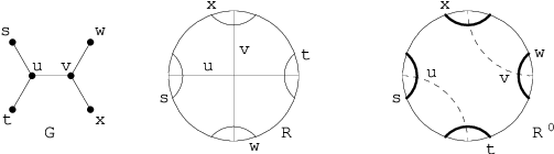
Circle Graphs. Circle graphs are intersection graphs of chords of a circle. They were first considered by Even and Itai [19] in the early 1970s in study of stack sorting techniques. Other motivations are due to their relations to Gauss words [18] (see Fig. 2\theletter) and matroid representations [17, 8]. Circle graphs are also important regarding rank-width [35].

Let denote the chromatic number of , and let denote the clique-number of . Trivially we have and the graphs for which every induced subgraph satisfies equality are the well-known perfect graphs [12]. In general, the difference between these two numbers can be arbitrarily high, e.g., there is a triangle-free graph with an arbitrary high chromatic number. Circle graphs are known to be almost perfect which means that for some function . The best known result for circle graphs [31] states that is and .
Some NP-hard problems, such as maximum weighted clique and independent set [22], become tractable on circle graphs. On the other hand, problems such as vertex colorability [21] and Hamiltonicity [16] remain NP-complete even for circle graphs.
The complexity of recognition of circle graphs was a long standing open problem; see [40] for an overview. The first results, e.g., [19], gave existential characterizations which did not give polynomial-time algorithms. The mystery whether circle graphs can be recognized in polynomial time frustrated mathematicians for some years. It was resolved in the mid-1980s and several polynomial-time algorithms were discovered [7, 20, 33] (in time and similar). Later, a more efficient algorithm [39] based on split decomposition was given, and the current state-of-the-art recognition algorithm [23] runs in a quasi-linear time in the number of vertices and the number of edges of the graph.
The Partial Representation Extension Problem. It is quite surprising that this very natural generalization of the recognition problem was considered only recently. It is currently an active area of research which is inspiring a deeper investigation of many classical graph classes. For instance, a recent result of Angelini et al. [1] states that the problem is decidable in linear time for planar graphs. On the other hand, Fáry’s Theorem claims that every planar graph has a straight-line embedding, but extension of such an embedding is NP-hard [36].
In the context of intersection-defined classes, this problem was first considered in [29] for interval graphs. Currently, the best known results are linear-time algorithms for interval graphs [5, 28] and proper interval graphs [26], a quadratic-time algorithm for unit interval graphs [26, 37, 38], and polynomial-time algorithms for permutation and function graphs [25], proper circular-arc graphs [3], and trapezoid graphs [32]. For chordal graphs (as subtree-in-a-tree graphs) several versions of the problems were considered [27] and all of them are NP-complete, and similarly for different contact representations of planar graphs [9]. In [30], minimal forbidden configurations making a partial interval representation non-extendible are characterized. Extending partial visibility representations is studied in [11].
The Structure of Representations. To solve the recognition problem for , one just needs to build a single representation. However, to solve the partial representation extension problem, the structure of all representations of must be well understood. A general approach used in the above papers is the following. We first derive necessary and sufficient constraints from the partial representation . Then we efficiently test whether some representation satisfies these constraints. If none satisfies them, then is not extendible. And if some satisfies them, then it extends .
It is well-known that the split decomposition [14, Theorem 3] captures the structure of all representations of circle graphs. The standard recognition algorithms produce a special type of representations using split decomposition as follows. We find a split in , construct two smaller graphs, build their representation recursively, and then join these two representations to produce . In Section 3, we give a simple recursive description of all possible representations based on splits. Our result can be interpreted as ‘‘describing a structure like PQ-trees11 1 See [6] for further information on PQ-trees. for circle graphs.” It is possible that the proof techniques from other papers on circle graphs such as [13, 23] would give a similar description. However, these techniques are more involved than our approach which turns out to be quite elementary and simple.
Restricted Representations. The partial representation extension problem belongs to a larger group of problems dealing with restricted representations of graphs. These problems ask whether there is some representation of an input graph satisfying some additional constraints. We describe two examples of these problems.
An input of the simultaneous representation problem22 2 Here, we will focus on what is sometimes referred to as the sunflower version in the literature, see [4]., shortly Sim, consists of graphs with some vertices common for all the graphs. The problem asks whether there exist representations representing the common vertices in the same way. This problem is polynomially solvable for permutation and comparability graphs [24]. They additionally show that for chordal graphs it is NP-complete when is part of the input and polynomially solvable for . For interval graphs, a linear-time algorithm is known for [5] and the complexity is open in general. For some classes, these problems are closely related to the partial representation extension problems. For example, there is an FPT algorithm for interval graphs with the number of common vertices as the parameter [29], and partial representations of interval graphs can be extended in linear time by reducing it to corresponding simultaneous representation problem [5].
The bounded representation problem [26] prescribes bounds for each vertex of the input graph and asks whether there is some representation satisfying these bounds. For circle graphs, the input specifies for each chord a pair of arcs of the circle, and a solution is required to have one endpoint of in and the other one in . This problem is clearly a generalization of partial representation extension since one can describe a partial representation using singleton arcs. It is known to be polynomially solvable for interval and proper interval representations of interval graphs [2], and surprisingly it is NP-complete for unit interval representations [26, 37, 38]. The complexity for other classes is not known.
Our Results. We study the following problem (see Section 2 for definitions):
| Problem: | Partial Representation Extension – |
|---|---|
| Input: | A circle graph and a partial representation . |
| Output: | Is there a representation of extending ? |
In Section 3, we describe a simple structure of all representations. This is used in Section 4 to obtain our main algorithmic result:
Theorem 0.1
The problem can be solved in time where is the number of vertices.
To spice up our results, we show in Section 5 the following for the simultaneous representation problem of circle graphs:
Theorem 0.2
If is a part of the input, the problem of circle graphs is NP-complete.
Finally, we show that Theorem 0.1 implies the following.
Corollary 0.1
The problem is FPT in the size of the common subgraph.
2 Definitions and Preliminaries
Circle Representations. A circle representation of a graph is a collection of chords of a circle such that intersects if and only if . A graph is a circle graph if it has a circle representation, and we denote the class of circle graphs by CIRCLE.
Notice that a representation of a circle graph is completely determined by the circular order of the endpoints of the chords in the representation, and two chords and cross if and only if their endpoints alternate in this order. For convenience we label both endpoints of the chord representing a vertex by the same label as the vertex.

Interval Overlap Graphs. Suppose that we cut the circle in a point which is not an endpoint of a chord and straighten it into a segment; see Fig. 3\theletter. From this straightening of the circle, each chord can now be seen as an arc above the resulting segment. Notice that two chords and cross if and only if their endpoints appear in the order or from left to right. Alternatively, circle graphs are called interval overlap graphs. Their vertices can be represented by intervals and two vertices are adjacent if and only if their intervals overlap which means they intersect and one is not a subset of the other.
Word representations. A sequence over an alphabet of symbols is a word. A circular word represents the set of words which are cyclical shifts of one another. In the sequel, we represent a circular word by a word from its corresponding set of words. We denote words and circular words by small Greek letters.
For a word and a symbol we write , if appears at least once in . Thus, is also used to denote the set of symbols occurring in . A word is a subword of , if appears consecutively in . A word is a subsequence of , if the word can be obtained from by deleting some symbols. We say that alternates with in , if or is a subsequence of . The corresponding definitions also apply to circular words. If and are two words, we denote their concatenation by .
The above interpretation of circle graphs as interval overlap graphs allows us to associate each representation of with a unique circular word over . The word is obtained by the circular order of the endpoints of the chords in as they appear along the circle when traversed clockwise. The occurrences of and alternate in if and only if . For example in Fig. 1\theletter corresponds to the circular word . Notice that each vertex appears exactly twice in . A circular subsequence of is induced by if is obtained from by deleting symbols in .
Partial Representations. Partial representations are defined in [29] and other papers as representations of induced subgraphs. In this paper, we consider the following more general definition. A partial representation of a circle graph is given by a circular word consisting of symbols of such that each appears at most twice in . A representation of corresponding to a circular word extends if and only if is a subsequence of . The endpoints in and the corresponding vertices are called pre-drawn. If a pre-drawn vertex has both occurrences in , the chord is pre-drawn.
3 Structure of Representations of Maximal Splits
Let be a connected graph. A split of is a partition of the vertices of into four parts , , and , such that:
-
We have and , but possibly or .
-
For every and , we have .
-
There is no edge between and , and between and .
Fig. 4\theletter shows two possible representations of a split. Notice that a split is uniquely determined just by the sets and , since consists of connected components of attached to , and of those attached to . We refer to this split as the split between and . Alternatively, a split between and is a cut in between and which is a complete bipartite graph.

The standard assumption is that a split is non-trivial, meaning that both sides of the split have at least two vertices: and . The reason is that trivial splits are not very interesting: in every graph , the choice and for forms a trivial split. The goal of split decomposition is to divide a graph into smaller graphs and trivial splits are not helpful.
One of the novelties of this paper is that we study maximal splits. A split of between and is maximal if there exists no split of between and such that , and or . Both splits between and and between and are allowed to be trivial. Maximal splits satisfy the following property:
Lemma 0.1
A split between and is maximal, if and only if there exists no connected component in such that each vertex of is either adjacent to all vertices of , or to none of them, and similarly for and .
Proof 3.3.
Suppose that such a component in exists, and let consists of those vertices which are adjacent to all vertices of . The split between and is not maximal since and forms a split, for which . Similarly, if such a component in exists, the split between and is not maximal.
On the other hand, suppose that a split between and is not maximal, so there exists a split between and such that, without loss of generality, and . Since every vertex of is adjacent to all vertices in , we have . Choose an arbitrary and let be its connected component of . As argued, all vertices of are adjacent to all vertices of . Since and , the remaining vertices . Therefore, they are non-adjacent to all vertices , and satisfies the properties from the statement of this lemma.
We always start with a non-trivial split between and , and modify it using Lemma 0.1 into a maximal split which may become trivial. But such a trivial maximal split has a special structure, described below:
Lemma 3.4.
Let and form a non-trivial split and let and form a trivial maximal split such that , , , and . Then is an articulation in , i.e., is disconnected.
Proof 3.5.
Since , we have . Since the split between and is non-trivial, we have . Therefore, is an articulation in which separates from .
In the rest of this section, we examine the recursive structure of every possible representation of based on maximal splits. In Section 3.1, we analyze the structure of a representation of a maximal split. In Section 3.2, we use it to describe the structure of all circle representations. The described results still apply to trivial maximal splits, but are not very helpful. Therefore, in Section 3.3, we give a different description of all representations based on trivial maximal splits.
3.1 Structure of a Representation of a Maximal Split
Let be a representation of a graph with a maximal split between and . The representation corresponds to a unique circular word . We consider the circular subsequence of induced by . The maximal subwords of consisting of vertices of alternate with the maximal subwords of consisting of vertices of . We denote all these maximal subwords according to their circular order; so . Without loss of generality, we assume that consists of symbols from . We call an -word when is odd, and a -word when is even.
We first investigate for each which symbols it contains.
Lemma 3.6.
For the subwords the following holds:
- (a)
Each contains each symbol at most once.
- (b)
The value of is even and the opposite words and contain the same symbols.
- (c)
Let . If and , then .
Proof 3.7.
(a) For every and , the fact implies that and alternate in the circular word . So if some contains both occurrences of, say, , then and would not alternate in .
(b) Let be, say, an -word. We first prove that all the other occurrences of the symbols from are contained in one word ; so we get a matching between the words. Suppose that this is not true and there is and for distinct and . There is at least one -word placed in between and (in the part of the circle not containing ). It is not possible for to alternate with both and , which contradicts .
Now, let and be two matched -words. Then every pair of matched -words must occur on opposite sides of the circle with respect to and . Therefore the same number of -words occur on both sides of and , and thus .
(c) This is implied by (a) and (b) since the occurrences of and alternate in .
Below, we prove that the structure of a maximal split between and greatly restricts possible representation of the vertices of :
Lemma 3.8.
Let and be defined as above. There exists a unique mapping satisfying the following properties:
- (a)
For , let be the subsequence of induced by . Then either , or is a subword of . For , the word is an -word, while for , it is a -word.
- (b)
For each connected component of , the mapping is constant, i.e., for all , we have , and we denote the image by .
Proof 3.9.
Without loss of generality, we assume that ; a symmetric argument works for . We first prove the existence and uniqueness of when is adjacent to some vertex in . Since alternates with , both and are non-empty. In (b), we prove that when , so by induction the existence and uniqueness follows for all vertices of .
(a) Since alternates with , if such exists, then it is an -word. Since -words and -words alternate in , we get that is a subword of some -word if and only if it contains no symbol from . Since at most one of and contains no symbol from , it is easy to see that such is unique. It remains to prove that it always exists.
Let be the connected component of containing . For contradiction, suppose that the property (a) fails for . If property (a) fails for , we have and such that , . Since , we also have ; see Fig. 5\theletter(a).

For each , we have , so induces in the subsequence such that both and consist only of symbols from . For each , we have and , so is adjacent to all vertices of . Since every vertex is connected by a path to , we have that induces in the subsequence , where both and consist of symbols of . Therefore every is either adjacent to all vertices of , or to none of them. By, Lemma 0.1, the split between and is not maximal.
(b) Let such that and is already determined. We want to prove that . As depicted in Fig. 5\theletter(b), let be the subsequence of induced by , and suppose that is a subword of . Both and cannot contain symbols from , otherwise alternates with and the argument in (a) applies. Therefore, either , or is a subword of , so . We note that either , or might be empty, so could be chosen arbitrarily to satisfy (a). We then set to also satisfy (b).
Let denote the subsequence of formed by , and of the symbols of over all connected components of . By Lemma 3.8, the only difference between and is that each subword is replaced by the subword which additionally contains all occurrences of the vertices in some connected components of or . Thus, .
Lemma 3.8 explains the following naming convention used for maximal splits between and in this paper; see Fig. 4\theletter. We call the vertices of and as long vertices with respect to the maximal split between and since each is represented by “long chords” between and . The vertices and are called short vertices with respect to the maximal split between and , because each is represented by “short chords” inside some . In the sequel, if the maximal split is clear from the context, we will just call some vertices long and some vertices short.
Lemma 3.10.
If two long vertices are connected by a path of length at least two having the internal vertices in , then and belong to the same pair and in every representation.
Proof 3.11.
Also, we prove the following simple lemma:
Lemma 3.12.
Let , , , and be distinct vertices inducing a clique in , and let be a path from to of length at least 2. If is a subsequence of the circular word of a circle representation of , then some internal vertex of is adjacent to or .
Proof 3.13.
Let be the internal vertices of such that . We prove by induction that no having or implies that . If is not such a vertex, then we get that is a subsequence of since . For the induction hypothesis, suppose that is a subsequence of . Since , if is not adjacent to and , we get that is a subsequence of . Therefore, does not alternate with , contradicting that .
3.2 Conditions Forced by a Maximal Split
Now, we want to investigate the opposite relation. Namely, what can one say about a representation from the structure of a maximal split? Suppose that and are two long vertices. We want to know the properties of and which force every representation to have a subword of containing both and .
Inspired by Naji [33, Section IV.4], we define a symmetric relation on where means that and must occur in the same subword of . This relation is given by two conditions:
- (C1)
Lemma 3.6(c) states that if , then , i.e., if and are placed in different subwords, then intersects . In particular, .
- (C2)
Lemma 3.10 gives when and are connected by a non-trivial path with all the inner vertices in .
Let us take the transitive closure of , which we denote by thereby slightly abusing the notation. Thus, we obtain an equivalence relation on . Notice that every equivalence class of is either fully contained in or in . Figure 4\theletter on right shows schematically a situation in which the relation has four equivalence classes , , and .
Now, let be an equivalence class of . We denote by the set consisting of all the vertices in the connected components of which have a vertex adjacent to a vertex of . Since satisfies (C2), we know that the sets of the equivalence classes of define a partition of .
Recognition Algorithms Based on Splits. Split decompositions are used in the current state-of-the-art algorithms for recognizing circle graphs. If a circle graph contains no split, it is called a prime graph. The representation of a prime graph is uniquely determined (up to the orientation of the circle) and can be constructed efficiently. There is an algorithm which finds a split in a graph in linear time [15]. In fact, the entire split decomposition tree (i.e., the recursive decomposition tree obtained via splits) can be found in linear time. Usually the representation is constructed as follows.
We define two graphs and where is created from by contracting the vertices of into a new vertex and by contracting into a new vertex . So is adjacent to all vertices in and to no vertices in , and similarly for . Then we apply the algorithm recursively on and and construct their representations and ; see Fig. 6\theletter. It remains to join the representations and in order to construct .

To this end we take and replace by the representation of in . More precisely, let the circular ordering of the endpoints of chords defined by be and let the circular ordering defined by be . The constructed has the corresponding circular ordering . It is easy to see that is a correct circle representation of .
Structure of All Representations. The above algorithm constructs a very specific representation of , and a representation like the one in Fig. 4\theletter on the right cannot be constructed in this way using the split between and . In what follows we describe the structure of all the representations of a circle graph based on the different circular orderings of the equivalence classes of . While the described structure of all the representations depends on the maximal split that we chose, the relation defined with respect to this maximal split can be used to generate all the representations of .
We choose an arbitrary circular ordering of the classes of . Let be a graph constructed from by contracting the vertices into one vertex ; i.e., is defined similarly to and above. Let be arbitrary representations of . We join these representations as follows. Let be the circular ordering of . We construct as the circular ordering
| (1\themathletter) |
In Fig. 4\theletter, we obtain the representation on the left by the circular ordering of the classes of and the representation on the right by .
First, we show that every representation obtained in this way is correct.
Lemma 3.14.
Every circular ordering (1\themathletter) constructed as above defines a circle representation of .
Proof 3.15.
Let . We shall prove that and are adjacent in if and only if they alternate in . Suppose that . Since the cyclic subsequence appears in both and , two vertices in alternate in if and only if they are adjacent in , which is if and only if they are adjacent in .
Otherwise, let and for . Then if and only if they are both long vertices. Each long vertex of appears once in both and , but each short vertex has both its occurrences either in , or in . We conclude that and alternate in if and only if they are both long vertices, i.e., if and only if they are adjacent in since and do not satisfy (C1).
Next, we analyze every representation of .
Lemma 3.16.
Let be the circular word corresponding to a representation of . Then the symbols of form exactly two subwords and of such that for each , we have and , while each has both endpoint either in , or in .
Proof 3.17.
Let be a representation of and consider how it represents . We get the subwords of the endpoints of , as described in Section 3.1.
Let such that . We claim that is a subset of . Since is an equivalence class of , let such that one of the conditions (C1) or (C2) applies to and . Since is the transitive closure of conditions (C1) and (C2), to prove the claim, it is sufficient to show that . If (C1) applies, then by Lemma 3.6(c). If (C2) applies, then by Lemma 3.10. By Lemma 3.6(a), each vertex of appears exactly once in and once in .
Furthermore, we claim that the vertices of form subwords of and . Let be placed between and . First, we assume that (C1) or (C2) applies to and .
-
If (C1) applies to and , then . As and do not alternate, it is not possible for to alternate with both and . Thus or , which in turn implies that .
-
Suppose that (C2) applies to and . If or , we get that by (C1). Otherwise, we claim that a path from to having all the internal vertices in has at least one internal vertex adjacent to . For every and , we have , but none of the inner vertices of are adjacent to . Since induce the subsequence in , by Lemma 3.12 some inner vertex has to alternate with . Thus, and by (C2), so .
If and neither of (C1) and (C2) applies, we easily proceed by an inductive argument on the number of applications of (C1) and (C2). If and a vertex is placed between and in , then is also placed in between and or between and .
By the above argument, each class forms two subwords of . By adding the short vertices as in Lemma 3.8 applied on the maximal split between and , we obtain two subwords of for each class .
Now, we are ready to prove the main structural proposition.
Proposition 3.18.
Let and form a maximal split of and let be the equivalence relation defined by (C1) and (C2) on . Then every representation of corresponds to some circular ordering and to some representations of . More precisely, can be constructed by arranging as in (1\themathletter): .
Proof 3.19.
By Lemma 3.14, every representation constructed by (1\themathletter) is correct. On the other hand, let be a representation of with the corresponding circular word . According to Lemma 3.16, we know that forms two subwords and of . For , the edges between and form a complete bipartite graph. The subwords , , and alternate, i.e., appear as or in . Thus, if we start from some point along the circle, the order of ’s gives a circular ordering of the classes. The representation has the circular word .
3.3 The Structure of All Representations of Trivial Maximal Splits
Let and form a trivial maximal split with and , created from a non-trivial split. The results described in Sections 3.1 and 3.2 still apply to this split, but they are not very helpful. By Lemma 3.4, is an articulation in . So, consists of at least two connected components and has two equivalence classes and . Since , Proposition 3.18 describes all representations of in terms of all representations of .
In this section, we show that all possible representations can be easily described in a different way, based on all different representations of connected components of . The following lemma states that connected components do not alternate in any circle representation:
Lemma 3.20.
Let and be two distinct connected component of a circle graph . No representation has a subword where and .
Proof 3.21.
Let be the subsequence induced by . We know that such that is the maximal subword consisting only of symbols from if is odd, and only of symbols from if is even. We want to prove that . For contradiction, suppose that . Since is connected, there exists such that and for . Since is connected, there exists such that and . Since and alternate, we have which is a contradiction.
We choose an arbitrary ordering of the connected components of as . Let be the subgraph of induced by . Let be an arbitrary representation of having the circular word . We construct the joined representation of by the circular word
| (2\themathletter) |
see Fig. 7\theletter. First, we prove that every such constructed representation of is correct:

Lemma 3.22.
Every circular ordering (2\themathletter) constructed as above defines a circle representation of .
Proof 3.23.
Let be the circular ordering constructed using (2\themathletter). Since induces the subsequence , each is represented correctly in . For , the vertices of induce in the subsequence , so no two vertices and alternate and the non-edges between and are represented correctly.
Next, we analyze every representation of .
Lemma 3.24.
Let be the circular word corresponding to a representation of . Then the symbols of form exactly two subwords and of such that is a subsequence of .
Proof 3.25.
Since , there exists some which alternates with , so the symbols of form at least two subwords alternating with . If would form more than two subwords, then has a subsequence , where and for . Since some alternates with , it follows that has the subsequence , so we get which is not possible by Lemma 3.20.
Now, we are ready to prove the following structural proposition.
Proposition 3.26.
Let and form a trivial maximal split of created from a non-trivial split. Then every representation of corresponds to some ordering of connected components of and to some representations of where is the subgraph of induced by . More precisely, can be constructed by arranging as in (2\themathletter): .
Proof 3.27.
By Lemma 3.22, every representation constructed by (2\themathletter) is correct. On the other hand, let be a representation of corresponding to a circular word . Suppose that has connected components. The circular word defines an ordering of the connected components of in the following way. By Lemma 3.24, , where and precisely one are two maximal subwords of containing all symbols from . Since the connected components cannot alternate by Lemma 3.20, we get that consists of symbols of , i.e., . Each gives some representation of .
4 Algorithm
In this section, we describe an algorithm for the partial representation extension problem of circle graphs. It is based on the structure of all representations of Section 3. Recall that a partial representation gives a circular word such that each vertex appears at most twice in . We want to decide whether there exists a representation corresponding to a circular word such that is a subsequence of .
Dealing with Disconnected Graphs. To apply the structural properties of Section 3, we need to work with connected graphs. In general, the partial representation extension problems cannot be trivially restricted to connected inputs, as in the case of most graph problems. In particular, for some classes the problems are polynomial-time solvable for connected inputs and FPT in the number of components for disconnected inputs, but NP-complete in general; see e.g. [26, 27]. The reason is that the components are placed together in one representation and they restrict each other.
In the case of circle graphs, we can deal with disconnected inputs easily. By Lemma 3.20, we know that cannot contain a subsequence where belong to one component and to another one. If this happens, we immediately output “no”. Otherwise the question of extendibility is equivalent to testing whether each component is extendible where the partial representation of is given by the subsequence of containing all occurrences of the vertices of . So from now on we assume that the input graph is connected.
Overview. Our algorithm proceeds recursively via split decomposition. For each encountered graph with a partial representation corresponding to the circular word , it proceeds with the following steps:
-
If is prime, we have two possible representations (one is reversal of the other) and we test whether one of them extends . We return the result.
-
Otherwise, we find a non-trivial split and modify it into a maximal split between and , using Lemma 0.1. Next, we proceed with one of the following steps.
-
In Case I, the maximal split between and is non-trivial. We compute the relation . We try to determine an ordering of the equivalence classes of along the circle as in (1\themathletter) which is compatible with the partial representation . This order is partially prescribed by pre-drawn endpoints of short and long vertices and we recurse on testing whether partial representations of different equivalence classes can be extended. If no ordering is compatible, we stop and output “no”.
-
In Case II, the maximal split between and is trivial with and . We try to determine an ordering of the connected components of along the circle as in (2\themathletter) which is compatible with the partial representation . This order is partially prescribed by pre-drawn endpoints of chords and we recurse on testing whether partial representations of different components can be extended. If no ordering is compatible, we stop and output “no”.
For a more detailed overview of the main steps, see Algorithm 1. Now we describe everything in detail.
| Input: A circle graph and a partial representation corresponding to a circular word . | |||||
| Output: ACCEPT if is extendible, REJECT otherwise. | |||||
| 1. | If | is incorrect then REJECT. | |||
| 2. | If is a prime graph then | ||||
| 3. | Construct the unique representations and (its reverse) of . | ||||
| 4. | If | is a subsequence of or then ACCEPT else REJECT. | |||
| 5. | Else ( is not a prime graph) | ||||
| 6. | Find a non-trivial split between and . | ||||
| 7. | Modify it into a maximal split between and such that and . | ||||
| 8. | Case I: If the maximal split between and is non-trivial then | ||||
| 9. | Compute the equivalence relation . | ||||
| 10. | Let be the maximal subwords of extended classes . | ||||
| 11. | Ca | se I.1: If some extended class corresponds to two maximal subwords in then | |||
| 12. | Compute a circular ordering compatible with . | ||||
| 13. | Construct the partial representations of . | ||||
| 14. | If all are extendible then ACCEPT else REJECT. | ||||
| 15. | Case I.2: Else (each extended class corresponds to one maximal subword in ) | ||||
| 16. | Construct the partial representations and of . | ||||
| 17. | Proceed as in the subroutine of Algorithm 2. | ||||
| 18. | Case II: Else (the maximal split between and is trivial with and ) | ||||
| 19. | Compute the connected components of . | ||||
| 20. | Case II.1: If both endpoints of appear in then | ||||
| 21. | Compute a linear ordering compatible with . | ||||
| 22. | Construct the partial representations of . | ||||
| 23. | If all are extendible then ACCEPT else REJECT. | ||||
| 24. | Case II.2: Else if single endpoint of appears in then | ||||
| 25. | Decompose the problem into two subproblems. | ||||
| 26. | One is solved using Case II.1, the other as in Case I.2. | ||||
| 27. | If both succeed then ACCEPT else REJECT. | ||||
| 28. | Case II.3: Else (no endpoint of appears in ) | ||||
| 29. | Ca | se II.3a: If some component has two maximal subwords in then | |||
| 30. | Decompose the problem into three subproblems. | ||||
| 31. | Two are solved using Case II.2, the last one using Case II.1. | ||||
| 32. | If all succeed then ACCEPT else REJECT. | ||||
| 33. | Else (no component has two maximal subwords in ) | ||||
| 34. | Proceed as in the subroutine of Algorithm 3. |
Testing Correctness of . In the beginning, the algorithm tests correctness of the input partial representation. If have both occurrences in , we check that these occurrences alternate if and only if , and if some pair is represented incorrectly, we stop the algorithm and output “no”. If only a single endpoint of appears in , no checking is done. This checking can be done trivially in time .
Prime Graphs. A graph is called prime if it contains no split. If is a prime graph, then it has at most two different representations and [15] where one is the reversal of the other. We just need to test whether one of them extends . We can construct one of these representations in quasilinear time [23].
Finding a Maximal Split Between and . If the graph is not prime, then we can find a non-trivial split between and in linear time [15]. Using Lemma 0.1, we modify it into a maximal split between and such that and in linear time.
4.1 Case I: A Non-trivial Maximal Split Between and .
We start by computing the equivalence relation which can be done in time . Next, we want to find an ordering of its equivalence classes. For a class of , we define the extended class of as . If some extended class has no vertex pre-drawn, we may choose an arbitrary representation and place it in an arbitrary order, so we can ignore such classes for the rest of Case I. Let have equivalence classes, all of them appearing in .
The circular word is composed of maximal subwords such that each contains only symbols of one extended class . According to Proposition 3.18, each extended class corresponds to at most two different maximal subwords. Also, if two extended classes and each correspond to two different maximal subwords, then occurrences of these subwords alternate in . Otherwise we reject the input.
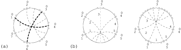
Case I.1: An extended class corresponds to two maximal subwords.
We denote this class by and put this class as first in the ordering. By renumbering, we may
assume that corresponds to and . Then one circular order of the classes
can be determined by the following linear ordering starting with . Let and
be two distinct classes. If corresponds to and corresponds to
such that either or , we put . We obtain the
ordering of the classes as any linear extension of . Since subwords of all extended classes with
two subwords in alternate, we get that is acyclic and a linear extension always exists.
Figure 8\theletter(a) shows an example.
We have ordered the extended classes and the corresponding classes . We construct each with the vertices as in Section 3.2, so is adjacent to and non-adjacent to . The partial representation of is either the word (if corresponds to the single maximal subword in ) or the word (if corresponds to two maximal subwords and in ). We test recursively, whether each representation of is extendible to a representation of . If yes, we join as in Proposition 3.18. Otherwise, the algorithm outputs “no”.
Lemma 4.28.
In Case I.1, the representation is extendible if and only if the representations of the graphs are extendible.
Proof 4.29.
Suppose that extends . According to Proposition 3.18, the representations of are ordered along the circle, and so we obtain representations extending .
For the other implication, we just take and combine them to form as in (1\themathletter). This works since the ordering was constructed so that extends .
Case I.2: No extended class corresponds to two maximal subwords.
We number the classes according to their appearance in , i.e., corresponds to the
subword . By Proposition 3.18, we know that in any representation
of the class corresponds to two subwords and . The difficulty here
arises from the potential for to be a subsequence of , but of neither
, nor . Figure 8\theletter(b) shows two potential extending representations.
We solve this as follows. Instead of constructing just one partial representation of corresponding to the circular word , we construct an additional partial representation corresponding to the circular word , i.e., has only one endpoint pre-drawn. Figure 9\theletter shows that is less restrictive: if is extendible, then is also extendible, but it might not be true the other way. For instance, every long chord in alternates with , so if some long chord has both endpoints pre-drawn in , is necessarily non-extendible, but might be extendible.
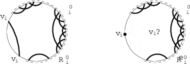
The following lemma is the main trick of the algorithm and is essential to prove that it has cubic running time. It states that, if is extendible, at most one class can be forced to use .
Lemma 4.30.
In Case I.2, the representation is extendible if and only if is extendible for some and is extendible for all .
Proof 4.31.
When corresponding to a word is an extension of for , then is a subsequence of, say, . On the other hand, when corresponding to a word is an extension of , then is a subsequence of , but might not be of or . We use the circular ordering of the classes and we construct the representation as in (1\themathletter):
where all pre-drawn endpoints of appear in those words written in bold. It is easy to see that extends since has no pre-drawn endpoints in .
For the other implication, suppose that extends . For contradiction, suppose that two distinct partial representations and are not extendible. According to Proposition 3.18, the representation gives a representation corresponding to of and corresponding to of . Since and are non-extendible, we have that is neither a subsequence of , nor , and similarly is neither of , nor . Therefore, either , or is a subsequence of , and we get that two maximal subwords in correspond to both and which is a contradiction.
| 1. Test whether each of is extendible. | |
| 2. If | two of are not extendible then REJECT. |
| 3. If exactly one of , denoted by , is not extendible then | |
| 4. | If and are extendible then ACCEPT else REJECT. |
| 5. Else (all of are extendible) | |
| 6. | If is extendible then ACCEPT else REJECT. |
Let and let be the largest class, so for . If we want to recursively test for each whether both and are extendible, the running time might be exponential since we might have . Fortunately, using Lemma 4.30, it is sufficient to test only one of and . We recursively test whether are extendible; see the pseudocode of Algorithm 2:
-
Two or more of are not extendible. By Lemma 4.30, is non-extendible, the algorithm stops and outputs “no”.
-
Exactly one of is not extendible. Let be the non-extendible representation. We test whether and are extendible. If at least one is non-extendible, the algorithm stops and outputs “no”. If both are extendible, we similarly join in the representations according to (1\themathletter) as described in the proof of Lemma 4.30.
-
All representations are extendible. We have representations where extends . We test whether the partial representation is extendible. If not, the algorithm stops and outputs “no”. If it extends, we get a representation of . We construct the representation using (1\themathletter) as described in the proof of Lemma 4.30.
Lemma 4.32.
In Case I.2, the representation is extendible if and only if the algorithm constructs it.
Proof 4.33.
We know that is extendible when is extendible. Lemma 4.30 states that is extendible if and only if at most one of is non-extendible while is extendible. The algorithm tests this in Case I.2, while postponing until it knows which of and needs to be tested.
4.2 Case II: A Trivial Maximal Split Between and
Let and . In Section 3.3 we characterized all possible representations in terms of representations of connected components of . We just need to test whether one of them is compatible with the partial representation corresponding to the circular word . Similarly as in Section 4.1, we may assume that every connected component has at least one endpoint in ; otherwise, we can deal with it trivially.
Case II.1: Both endpoints of appear in . The circular word is composed of and maximal subwords such that each contains only symbols of one connected component and similarly for each . According to Proposition 3.26, each connected component corresponds to at most two different maximal subwords. If a connected component corresponds to two subwords and , then is a subsequence of . Also, if two components and each correspond to two different maximal subwords, then occurrences of these subwords do not alternate in . Otherwise we reject the input.
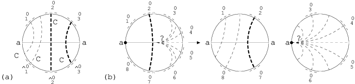
Next, we find a linear ordering of connected components as follows. We order if corresponds to a subword and to a subword for , or to and to for . We obtain a linear ordering as any linear extension. Since subwords of all connected components with two subwords in do not alternate, we get that is acyclic and a linear extension always exists. Suppose that we renumber the maximal subwords of in such a way that corresponds to and (one of them possibly empty). Let be the subgraph of induced by . Let be the partial representation of corresponding to the circular word , so . Figure 10\theletter(a) shows an example.
Lemma 4.34.
In Case II.1, the representation is extendible if and only if the representations of the graphs are extendible.
Proof 4.35.
Suppose that extends . According to Proposition 3.26, the representations of are ordered along the circle, and so we obtain representations extending .
For the other implication, we just take and combine them to form as in (2\themathletter). This works since the ordering was constructed so that extends .
Case II.2: A single endpoint of appears in . The circular word is composed of maximal subwords such that each contains only symbols of one connected component . According to Proposition 3.26, each connected component corresponds to at most two different maximal subwords. Also, if two components and each correspond to two different maximal subwords, then occurrences of these subwords do not alternate in . Otherwise we reject the input.
Suppose there is a component corresponding to two maximal subwords and for . Further let be such a component that maximizes the value . In every extending representation, we have the subsequence , so we can assume that the second endpoint of is pre-drawn in between and . We divide testing whether is extendible into two subproblems. We deal with the connected components of the circular word exactly as in Case II.1. It remains to decide whether is extendible where each connected component corresponds to precisely one maximal subword (note: when no such component exists, we have precisely this situation). Figure 10\theletter(b) shows an example.
Suppose that we rename such that corresponds to the connected component . Similarly to Case I.2, the difficulty comes from the fact that some might be a subsequence of of (2\themathletter) in an extending representation, but not of or . We consider two partial representations for each : the partial representation corresponding to and corresponding to . Again, if is extendible, then is also extendible.
Lemma 4.36.
In Case II.2 with no connected component correspond to two maximal subwords of , the representation is extendible if and only if is extendible for some and is extendible for all .
Proof 4.37.
When corresponding to a word is an extension of for , then is a subsequence of, say, for and of for . On the other hand, when corresponding to a word is an extension of , then is a subsequence of , but might not be of or . We use the linear ordering of the connected components and we construct the representation as in (2\themathletter):
where all pre-drawn endpoints of appear in those words written in bold. It is easy to see that extends since there are no pre-drawn endpoints in and in .
For the other implication, suppose that corresponding to extends , and we add into the position of the other endpoint of . It splits at most one maximal word , so is a subsequence of and is extendible. Since is a subsequence of , we get that is extendible.
The rest of this case proceeds exactly as Case I.2.
Lemma 4.38.
In Case II.2, the representation is extendible if and only if the algorithm constructs it.
Proof 4.39.
The proof is similar to Lemma 4.32.
Case II.3: No endpoint of appears in . As in Case II.2, the circular word is composed of maximal subwords . If two components and each correspond to two different maximal subwords, then occurrences of these subwords do not alternate in . Otherwise we reject the input. Also, if some connected component corresponds to two subwords and , then is a subsequence of every extending representation. Therefore, existence of such a component restricts the possible positions of endpoints of , so we divide this case into two subcases.
Case II.3a: Some component has two maximal subwords in . By a suitable renaming of the subwords, let be the connected component corresponding to and such that , is minimal, and correspond to connected components having only one maximal subword in . Similarly, let be the connected component corresponding to and such that and all correspond to connected components having only one maximal subword in , and possibly . If is extendible, we get that every connected component corresponding to two maximal subwords and has ; otherwise we reject the input. Figure 11\theletter shows an example.
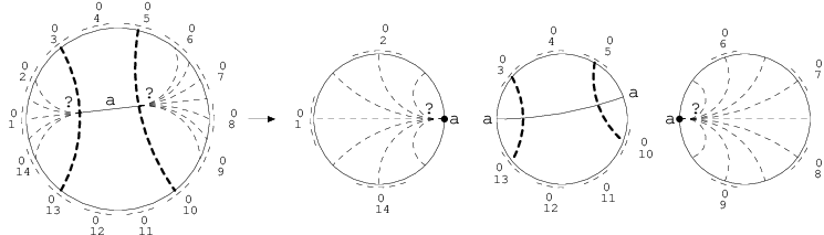
It follows that every extending representation has as a subsequence. Similarly as Case II.2, we can divide testing whether is extendible into three subproblems:
-
Testing using Case II.2 whether the partial representation is extendible.
-
Testing using Case II.1 whether the partial representation is extendible.
-
Testing using Case II.2 whether the partial representation is extendible.
Lemma 4.40.
In Case II.3a, the representation is extendible if and only if the algorithm constructs it.
Case II.3b: No component has two maximal subwords in . Let correspond to the connected component , and define and exactly as in Case II.2. Similarly to Case II.2, the difficulty comes from the fact that some might correspond to both and of (2\themathletter) in an extending representation. Since we are placing two endpoints of , we might have two such components and .
Lemma 4.42.
The representation is extendible if and only if and are extendible for some and , and is extendible for all .
Proof 4.43.
Let . When corresponding to a word is an extension of for , then is a subsequence of, say, for and of for . On the other hand, when corresponding to a word is an extension of , then is a subsequence of , but might not be of or , and similarly for . We use the linear ordering of the connected components and we construct the representation as in (2\themathletter):
where all pre-drawn endpoints of appear in those words written in bold. It is easy to see that extends since there are no pre-drawn endpoints in , in , and in .
For the other implication, suppose that corresponding to extends , and we add into the positions of the endpoints of . It is not possible that both endpoints split the same maximal word , otherwise the remaining components would alternate with . It is additionally not possible that two maximal words are split by the same endpoint. So at most two maximal words and are split by the endpoints of . Therefore, for every , we have as a subsequence of , so is extendible. Since and are subsequences of , we get that and are also extendible.
Let and let be the largest component, so for . The algorithm works similarly to Case I.2; see Algorithm 3 for a pseudocode. So we test the extendibility of only one of and while testing both types of representations for at most two other graphs and .
| 1. Test whether each of is extendible. | |
| 2. If | three of are not extendible then REJECT. |
| 3. If exactly two of , denoted and , are not extendible then | |
| 4. | If , and are extendible then ACCEPT else REJECT. |
| 5. If exactly one of , denoted , is not extendible then | |
| 6. | If and are extendible then ACCEPT else REJECT. |
| 7. Else (all of are extendible) | |
| 8. | If is extendible then ACCEPT else REJECT. |
Lemma 4.44.
In Case II.3b, the representation is extendible if and only if the algorithm constructs it.
4.3 Analysis of the Algorithm
By using the established results, we show that the partial representation extension problem of circle graphs can be solved in cubic time.
Lemma 4.46.
The described algorithm correctly decides whether the partial representation of is extendible.
Proof 4.47.
If the input graph is prime, we just test both representations whether they extend . If the input graph contains a non-trivial split, we modify it into a maximal split between and using Lemma 0.1. Next, we proceed by Case I or Case II, depending whether the maximal split is trivial or not. For Case I, the algorithm is correct by Lemmas 4.28 and 4.32. For Case II, the algorithm is correct by Lemmas 4.34, 4.38, 4.40, and 4.44.
Lemma 4.48.
The running time of the algorithm is where is the number of vertices.
Proof 4.49.
Let denote the time complexity of the algorithm for at most vertices in the worst case. We want to show that .
As described, we can test whether the graph is prime and construct a unique representation in quasilinear time using [23], but for the purpose of our analysis is sufficient. Since each symbol appears twice in , we can easily test in linear time whether is a subsequence of or its reversal. If is not prime, then we can find a non-trivial split between and using [15] and modify it using Lemma 0.1 into a maximal split between and such that and . Both can be achieved in linear time.
Case I. We compute the relation in time .
-
In Case I.1, we divide the problem into smaller disjoint subproblems of total size , each of size solvable by induction hypothesis in time , so the total running time is .
-
In Case I.2, we test both representations and for at most one extended class of size , while we test exactly one of these representations of all remaining extended classes. We get the following recursion:
By the Master Theorem, we get that . Since the depth of the recursion is at most linear, each level of the recursion adds to at most and we get in total over all levels.
Case II. We find connected components of in linear time.
-
In Case II.1, the analysis is similar as in Case I.1.
-
In Case II.2, we divide the input into two disjoint subproblems, one is solved as in Case II.1, the other as in Case I.2. Therefore, the total running time is .
-
In Case II.3a, we divide the input into three disjoint subproblems solved using Case II.1 and Case II.2, so the total running time is .
-
In Case II.3b, we test both representations and for at most two extended class of size , while we test exactly one of these representations of all remaining extended classes. We get the following recursion:
By the Master Theorem, we again get that .
Therefore, the total running time is .
The proof of the main result in this paper now follows easily.
5 Simultaneous Representations of Circle Graphs
In this section, we give two results concerning the simultaneous representation problem for circle graphs: We show that this problem is NP-complete and FPT in the size of the common intersection. Formally, we deal with the following decision problem:
| Problem: | Simultaneous Representation for Circle Graphs – |
|---|---|
| Input: | Graphs such that for all . |
| Output: | Do there exist representations of which use the same representation of the vertices of ? |
Proof 5.51 (Proof of Theorem 0.2).
To show that is NP-complete, we reduce it from the total ordering problem:
| Problem: | The total ordering problem - TotalOrdering |
|---|---|
| Input: | A finite set and a finite set of triples from . |
| Output: | Does there exist a total ordering of such that for all either , or ? |
Opatrny [34] proved this problem is NP-complete.
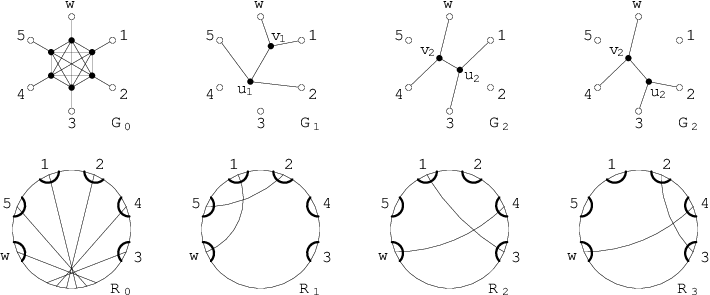
Given an instance of TotalOrdering and let and . We construct a set of graphs as follows, so the number from is equal . The intersection of is an independent set where is a special vertex. The graph consists of a clique , and to each vertex of this clique we attach exactly one vertex of as a leaf. The graph corresponds to the -th constraint . In addition to , each contains two vertices and of degree three, such that is adjacent to , and , and is further adjacent to and the special vertex . See Fig. 12\theletter for an example of this construction.
The clique in defines a split where each class of is a singleton. According to Proposition 3.18, every representation of places the elements of in some circular ordering which corresponds to the total ordering . Now the representations of can be constructed if and only if all the total ordering constraints are satisfied. This implies that there exists a solution of if and only if the instance of TotalOrdering is solvable.
Further, we show that the problem is FPT in size of the common subgraph .
Proof 5.52 (Proof of Corollary0.1).
We just consider all possible representations of the common subgraph which are all words of length . Each word gives some partial representation . We just solve instance of for each and the partial representation of , which can be done in polynomial time according to Theorem 0.1.
6 Conclusions
The structural results described in Section 3, namely Propositions 3.18 and 3.26, are the main new tools developed in this paper. Using it, one can easily work with the structure of all representations which is a key component of the algorithm of Section 4 that solves the partial representation extension problem for circle graphs. The algorithm works with the recursive structure of all representations and matches the partial representation on it. Proposition 3.18 also seems to be useful in attacking the following open problems:
Question 6.53.
What is the complexity of for a fixed number of graphs? In particular, what is it for ?
Recall that in the bounded representation problem, we give for some chords two circular arcs and we want to construct a representation which places endpoints into these circular arcs.
Question 6.54.
What is the complexity of the bounded representation problem for circle graphs? This question is also open for interval graphs and proper interval graphs.
Permutation Graphs. Permutation graphs are intersection graphs of segments between two parallel lines. So every permutation representation of consists of two words and , each containing each vertex exactly once, and if and only if their order in and differs. We denote the class by PERM.
Let be the reversal of . Since is a circle representation of , it follows that every permutation graph is a circle graph. More strongly, a graph is a permutation graph if and only if constructed from by adding a universal vertex is a circle graph, since is a circle representation of .
The partial representation problem for permutation graphs is studied in [25] and solved in time . The following results gives an alternative algorithm running in time as well.
Proposition 6.55.
The problem reduces in time to .
Proof 6.56.
Let be a permutation graph with a partial representation corresponding to two words and . The problem asks whether there exists words and representing such that and are subsequences of and , respectively. The reduction constructs the circle graph by adding a universal vertex to and the partial representation given by the circular word . The reduction clearly works in linear time. It is correct since the partial representation of is extendible if and only if of is extendible.
Minimal Split Decomposition and Split Trees. A split decomposition of works as follows. Consider a split between and . We replace by the graphs and defined in Section 3.2. Then we apply the decomposition recursively on and , and we stop on prime graphs containing no splits. We note that by different orders of splits, different decompositions of may be constructed. A split decomposition can be computed in linear time [15].
A split decomposition is called minimal if it is constructed by the least number of splits. Suppose that we also stop on degenerate graphs which are complete graphs and stars . Cunningham [14, Theorem 3] proved that the minimal split decomposition of a connected graph stopping on prime and degenerate graphs is unique.

The unique split tree representing a graph encodes the minimal split decomposition [23]. A split tree is a graph with two types of vertices (normal and marker vertices) and two types of edges (normal and tree edges). We initially put and modify it according to the minimal split decomposition. If the minimal decomposition contains a split between and in , then we replace in by the graphs and , and connect the marker vertices and by a tree edge (see Fig. 13\thelettera). We repeat this recursively on and ; see Fig. 13\theletterb. Each prime and degenerate graph is a node of the split tree. A node that is incident with exactly one tree edge is called a leaf node.
The minimal split decompositions and the split trees can be computed in quasi-linear time [23]. Similarly as in Propositions 3.18 and 3.26, it should be possible to derive every circle representation of a connected graph from the split tree , but the precise statement is unclear. It is a natural question whether split trees can be used to solve the partial representation extension problem:
Question 6.57.
Is it possible to use split trees to solve ? Can it be done faster that in time ?
We want to thank to an anonymous reviewer for pointing out than the results described in Section 3 work only for maximal splits.
The second author is supported by the People Programme (Marie Curie Actions) of the European Union’s Seventh Framework Programme (FP7/2007-2013) under REA grant agreement no [291734].
The third author is supported by CE-ITI (P202/12/G061 of GAČR) and Charles University as GAUK 1334217.
extending_circle_graphs
References
- [1] P. Angelini, G. D. Battista, F. Frati, V. Jelínek, J. Kratochvíl, M. Patrignani, and I. Rutter. Testing planarity of partially embedded graphs. ACM Trans. Algorithms, 11(4):32:1–32:42, 2015.
- [2] M. Balko, P. Klavík, and Y. Otachi. Bounded representations of interval and proper interval graphs. In ISAAC, volume 8283 of Lecture Notes in Computer Science, pages 535–546, 2013.
- [3] J. Bang-Jensen, J. Huang, and X. Zhu. Completing orientations of partially oriented graphs. CoRR, abs/1509.01301, 2015.
- [4] T. Bläsius, S. G. Kobourov, and I. Rutter. Simultaneous embedding of planar graphs. In Roberto Tamassia, editor, Handbook of Graph Drawing and Visualization, pages 349–383. CRC Press, 2013.
- [5] T. Bläsius and I. Rutter. Simultaneous PQ-ordering with applications to constrained embedding problems. ACM Trans. Algorithms, 12(2):16:1–16:46, 2015.
- [6] K. S. Booth and G. S. Lueker. Testing for the consecutive ones property, interval graphs, and planarity using PQ-tree algorithms. Journal of Computational Systems Science, 13:335–379, 1976.
- [7] A. Bouchet. Reducing prime graphs and recognizing circle graphs. Combinatorica, 7(3):243–254, 1987.
- [8] A. Bouchet. Unimodularity and circle graphs. Discrete Mathematics, 66(1-2):203–208, 1987.
- [9] S. Chaplick, P. Dorbec, J. Kratochvíl, M. Montassier, and J. Stacho. Contact representations of planar graphs: Extending a partial representation is hard. In WG’14, volume 8747 of Lecture Notes in Computer Science, pages 139–151. 2014.
- [10] S. Chaplick, R. Fulek, and P. Klavík. Extending partial representations of circle graphs. In Graph Drawing, volume 8242 of Lecture Notes in Computer Science, pages 131–142. 2013.
- [11] S. Chaplick, G. Guśpiel, G. Gutowski, T. Krawczyk, and G. Liotta. The partial visibility representation extension problem. In Graph Drawing and Network Visualization: 24th International Symposium, GD 2016, volume 9801 of Lecture Notes in Computer Science, pages 266–279, 2016.
- [12] M. Chudnovsky, N. Robertson, P. Seymour, and R. Thomas. The strong perfect graph theorem. Annals of Mathematics, 164:51–229, 2006.
- [13] B. Courcelle. Circle graphs and monadic second-order logic. J. Applied Logic, 6(3):416–442, 2008.
- [14] W. Cunningham. Decomposition of directed graphs. SIAM J. Alg. and Disc. Methods, 3:214–228, 1982.
- [15] E. Dahlhaus. Parallel algorithms for hierarchical clustering and applications to split decomposition and parity graph recognition. Journal of Algorithms, 36(2):205–240, 1998.
- [16] P. Damaschke. The hamiltonian circuit problem for circle graphs is NP-complete. Information Processing Letters, 32(1):1–2, 1989.
- [17] H. de Fraysseix. Local complementation and interlacement graphs. Discrete Mathematics, 33(1):29–35, 1981.
- [18] H. de Fraysseix and P. O. de Mendez. On a characterization of gauss codes. Discrete & Computational Geometry, 22(2):287–295, 1999.
- [19] S. Even and A. Itai. Queues, stacks, and graphs. Theory of Machines and Computation (Z. Kohavi and A. Paz, Eds.), pages 71–76, 1971.
- [20] C. P. Gabor, K. J. Supowit, and W. Hsu. Recognizing circle graphs in polynomial time. J. ACM, 36(3):435–473, 1989.
- [21] M. Garey, D. Johnson, G. Miller, and C. Papadimitriou. The complexity of coloring circular arcs and chords. SIAM Journal on Algebraic Discrete Methods, 1(2):216–227, 1980.
- [22] F. Gavril. Maximum weight independent sets and cliques in intersection graphs of filaments. Information Processing Letters, 73(5-6):181–188, 2000.
- [23] E. Gioan, C. Paul, M. Tedder, and D. Corneil. Practical and efficient circle graph recognition. Algorithmica, 69(4):759–788, 2014.
- [24] K. R. Jampani and A. Lubiw. The simultaneous representation problem for chordal, comparability and permutation graphs. Journal of Graph Algortihms and Applications, 16(2):283–315, 2012.
- [25] P. Klavík, J. Kratochvíl, T. Krawczyk, and B. Walczak. Extending partial representations of function graphs and permutation graphs. In Leah Epstein and Paolo Ferragina, editors, Algorithms – ESA 2012, volume 7501 of LNCS, pages 671–682. 2012.
- [26] P. Klavík, J. Kratochvíl, Y. Otachi, I. Rutter, T. Saitoh, M. Saumell, and T. Vyskočil. Extending partial representations of proper and unit interval graphs. Algorithmica, 77(4):1071–1104, 2017.
- [27] P. Klavík, J. Kratochvíl, Y. Otachi, and T. Saitoh. Extending partial representations of subclasses of chordal graphs. Theoretical Computer Science, 576:85–101, 2015.
- [28] P. Klavík, J. Kratochvíl, Y. Otachi, T. Saitoh, and T. Vyskočil. Extending partial representations of interval graphs. Algorithmica, 78(3):945–967, 2017.
- [29] P. Klavík, J. Kratochvíl, and T. Vyskočil. Extending partial representations of interval graphs. In Mitsunori Ogihara and Jun Tarui, editors, Theory and Applications of Models of Computation, volume 6648 of LNCS, pages 276–285. 2011.
- [30] P. Klavík and M. Saumell. Minimal obstructions for partial representations of interval graphs. In ISAAC, volume 8889 of Lecture Notes in Computer Science, pages 401–413, 2014.
- [31] A. Kostochka and J. Kratochvíl. Covering and coloring polygon-circle graphs. Discrete Mathematics, 163(1-3):299–305, 1997.
- [32] T. Krawczyk and B. Walczak. Extending partial representations of trapezoid graphs. In WG 2017, Lecture Notes in Computer Science, 2017.
- [33] W. Naji. Graphes de Cordes: Une Caracterisation et ses Applications. PhD thesis, l’Université Scientifique et Médicale de Grenoble, 1985.
- [34] J. Opatrny. Total ordering problem. SIAM J. on Computing, 8(1):111–114, 1979.
- [35] S. Oum. Rank-width and vertex-minors. J. Comb. Theory, Ser. B, 95(1):79–100, 2005.
- [36] M. Patrignani. On extending a partial straight-line drawing. In Patrick Healy and Nikola S. Nikolov, editors, Graph Drawing, volume 3843 of LNCS, pages 380–385. 2006.
- [37] F. J. Soulignac. Bounded, minimal, and short representations of unit interval and unit circular-arc graphs. Chapter I: theory. J. Graph Algorithms Appl, 21(4):455–489, 2017.
- [38] F. J. Soulignac. Bounded, minimal, and short representations of unit interval and unit circular-arc graphs. Chapter II: algorithms. J. Graph Algorithms Appl, 21(4):491–525, 2017.
- [39] J. P. Spinrad. Recognition of circle graphs. J. of Algorithms, 16(2):264–282, 1994.
- [40] J. P. Spinrad. Efficient Graph Representations. Field Institute Monographs, 2003.