Fault detection and isolation of malicious nodes
in MIMO Multi-hop Control Networks

Wireless networked control systems are spatially distributed control systems where the communication between sensors, actuators, and computational units is supported by a wireless multi-hop communication network. The use of wireless Multi-hop Control Networks (MCNs) in industrial automation results in flexible architectures and generally reduces installation, debugging, diagnostic and maintenance costs with respect to wired networks. Although MCNs offer many advantages, co-design of the network configuration and of the control algorithm for a MCN requires addressing the joint dynamics of the plant and of the communication protocol.

Recently, a huge effort has been made in scientific research on Networked Control Systems (NCSs), see e.g. [2], [25], [11], [24], [10], [8], [14] and references therein for a general overview. In general, the literature on NCSs addresses non–idealities (such as quantization errors, packets dropouts, variable sampling and delay and communication constraints) as aggregated network performance variables, losing irreversibly the dynamics introduced by scheduling and routing communication protocols. What is needed for modeling and analyzing control protocols on MCNs is an integrated framework for analysing/co-designing network topology, scheduling, routing and control. In [1], a simulative environment of computer nodes and communication networks interacting with the continuous-time dynamics of the real world is presented. To the best of our knowledge, the first formal model of a Multi-hop Control Network has been presented in [18, 19], where a mathematical framework has been proposed that allows modeling the MAC layer (communication scheduling) and the Network layer (routing) of recently developed wireless industrial control protocols, such as WirelessHART and ISA-100. In [5] we extended the formalism proposed in [19] by defining a MCN $\mathcal{M}$, that consists of a continuous-time SISO LTI plant $\mathcal{P}$ interconnected to a controller $C$ via two (wireless) multi-hop communication networks $G_{\mathcal{R}}$ (the controllability network) and $G_{\mathcal{O}}$ (the observability network), as illustrated in Figure 1, and by modeling redundancy in data communication - i.e. sending actuation/sensing data via multiple paths and then merging these components according to a weight function. This approach, which can be interpreted as a form of network coding at the level of the application layer of the ISO/OSI protocol stack, is called multi-path routing (or flooding, in the communication scientific community) and aims at enabling the detection and isolation of node failures and malicious intrusions, which cannot be done using single-path routing or strategies that use timestamps to discard redundant packets. It is well known that redundancy can also render the system fault-tolerant with respect to node failures and mitigate the effect of packet losses. We remark that, as illustrated in [16], the implementation of multi-path routing in a Wireless HART device only requires a minor change which retains backward compatibility with standard devices.

Paper contribution: Because of wireless networking, a MCN can be subject to failures and/or malicious attacks. In [5] we addressed and solved the problem of designing a set of controllers and the communication protocol parameters of a SISO MCN, so that it is possible to detect and isolate the faulty nodes of the controllability and observability networks and apply an appropriate controller to stabilize the system, as depicted in Figure 1. In [21] and in this paper we extend such investigation to MIMO MCNs: in particular, while in [21] we extended the MCN formalism to MIMO LTI plants and developed a procedure to guarantee the existence of a stabilizing controller $C_{i}$ for any node failure, in this paper we provide conditions on network topology, scheduling and routing that enable detection and isolation of node failures.

The extension with respect to the results in [5] is not trivial: indeed in the MIMO case the geometric approach exploited in [5] does not easily provide a relation between the conditions that enable FDI of node failures and the network topology, scheduling and routing. To overcome this issue we exploit formalism and FDI methodologies of structured systems [9]. This methodology leverages on the classical observer-based results in [12], where the system with failures is required to be left-invertible: therefore our results imply that almost any failure signal can be detected and isolated. In order to detect and isolate any non-zero failure signal we should require input-observability. Indeed a carefully chosen (malicious) failure may hide in the zero dynamics, being therefore undetectable: for example in [23, 17] the role of invariant zeros in detecting malicious attacks has

Related work: As can be inferred from the recent survey [7], fault tolerant control and fault diagnosis is one of the main issues addressed in the research on NCSs. However, most of the existing literature does not consider the effect of the communication protocol introduced by a Multi-hop Control Network. In [4], a procedure to minimize the number and cost of additional sensors, required to solve the FDI problem for structured systems, is presented. In [20] the design of an intrusion detection system is presented for a Wireless Control Network: our work differs from such results in the following four aspects. (1) In [13] the wireless network is an autonomous system where the network itself acts as a decentralized controller, while in our model the wireless network transfers sensing and actuation data between a plant and a centralized controller, namely it acts as a relay network. This modeling choice is motivated by the fact that WirelessHART and ISA-100 are designed for control loops where a centralized controller exploits a wireless network to relay sensing and actuation data, which is often a forced choice in industrial environments. (2) As a consequence of the previous issue, in [13] FDI is performed only exploiting the output signal from a subset of communication nodes, while we can exploit the input and output signals of the centralized controller. (3) In our model we take into account the effect of the scheduling ordering of the node transmissions in the sensing and actuation data relay, which provides a more accurate modeling of the effect of scheduling on the closed loop dynamics. Indeed, the conditions we derive in Section V show that, in order to guarantee FDI of faulty nodes, the link scheduling order is irrelevant: this is an interesting result because, as widely discussed in [6, 5, 22], it strongly reduces the scheduling period, avoids the necessity of on-the-fly scheduling re-definition, and always guarantees the existence of an admissible scheduling when multiple loops exploit the same communication network. (4) In [20] FDI is performed by on-the-fly testing the rank of a number of matrices which is a combinatorial function of the number of communication links, while our method only requires to apply a logic operator to a number of Luenberger observers which is at most equal to the number of communication nodes. To the best of our knowledge, our work is pioneering in addressing FDI for a MCN that implements standardized communication protocols. An extended version of this paper can be found on ArXiv.

Notation: We will denote by $\mathbb{N}$ and $\mathbb{R}$ respectively the sets of natural and real numbers. Given $n\in\mathbb{N}$, we denote by $\mathbb{n}$ the set $\mathbb{n}\doteq\{1,2,\ldots,n\}$. We denote by $\textbf{0}_{n\times m}$ the matrix of zeros with $n$ rows and $m$ columns and by $\textbf{I}_{n}$ the identity matrix of dimension $n$. Given a finite set $A$ and a subset $B\subseteq A$, we define $|A|$ and $|B|$ their cardinality, $A\setminus B$ the difference set and $2^{A}$ the power set. We denote by $diag(F_{1}(z),\ldots,F_{n}(z))$ the $n\times n$ diagonal transfer function matrix whose diagonal consists of the scalar transfer functions $F_{1}(z),\ldots,F_{n}(z)$. Given a directed graph $(\mathcal{V},\mathcal{E})$ we define path an alternating sequence of vertices and edges. A path is defined simple if no vertices are repeated. We define a set of paths vertex disjoint if each two of them consist of disjoint sets of vertices. We call a set of $r$ disjoint and simple paths from a set $\mathcal{V}_{1}\subseteq\mathcal{V}$ to a set $\mathcal{V}_{2}\subseteq\mathcal{V}$ an $r$-linking from $\mathcal{V}_{1}$ to $\mathcal{V}_{2}$. We denote by $\biguplus$ the disjoint union operator among directed graphs. For a formal definition of further graph properties and notations (e.g. weakly connected graph, weakly connected component, bridge nodes etc.) the reader is referred to [26].

We propose a mathematical framework for modeling wireless multi-hop communication networks that implement time-triggered protocols such as WirelessHART and ISA-100. In these standards the access to the shared communication channel is specified as follows: time is divided into slots of fixed duration $\Delta$ and groups of $\Pi$ time slots are called frames of duration $T=\Pi\Delta$ (see Figure 2). For each frame, a communication scheduling allows each node to transmit data only in a specified time slot. The scheduling is periodic with period $\Pi$, i.e. it is repeated in all frames.

The main difference with respect to the MCN definition given in [15] for SISO systems is that here the network needs to relay $m$ actuation signals and $\ell$ sensor signals: we assume that nodes routes data of each of these signals separately.

Designing a scheduling function induces a communication scheduling (namely the time slot when each node is allowed to transmit) and a multi-path routing (namely the set of paths that convey data from the input to the output of the connectivity graph) of the communication protocol. Since the scheduling function is periodic, the induced communication scheduling is periodic and the induced multi-path routing is static.

$G_{\mathcal{R}}(\eta_{\mathcal{R}_{i}})$ consists of a set of simple (routing) paths starting from $v_{u,c}$ and terminating in $v_{u,i}$. As a consequence $G_{\mathcal{R}}(\eta_{\mathcal{R}_{i}})$ is a directed, weakly connected and acyclic graph. The above definition can be given similarly for $G_{\mathcal{O}}$ and $\eta_{\mathcal{O}_{i}}$.

Nominal MCN: The dynamics of a MCN $\mathcal{M}$ can be modeled by the interconnection of blocks as in Figure 3. The block $\mathcal{P}$ is characterized by the discrete-time transfer function matrix $\mathcal{P}(z)$ obtained by discretizing the system $\mathcal{P}$ with sampling time ${T}=\Pi\Delta$. The block $\mathcal{R}$ models the dynamics introduced by the flow of the actuation data of all components of the control input $u$ via the communication network represented by $G_{\mathcal{R}}$. In order to define the dynamics of $\mathcal{R}$, we need to define the semantics of the data flow through the network induced by the scheduling and the weight functions. We assume that each communication node, when scheduled to transmit by $\eta_{\mathcal{R}_{i}}$, computes a linear combination of the data associated to the input component $u_{i}$ and received from the incoming links according to the weight function $W_{\mathcal{R}_{i}}$. This linear combination is then transmitted via the outgoing scheduled links. As in [21] the input/output behavior of $u_{i}(kT)$ with respect to $\tilde{u}_{i}(kT)$ can be formalized, for any $i\in\mathbb{m}$, by the following transfer function:

where $D_{\mathcal{R}_{i}}\in\mathbb{N}$ is the maximum delay introduced by the (routing) paths of $G_{\mathcal{R}}(\eta_{\mathcal{R}_{i}})$ and $\forall d\in\boldsymbol{D_{\mathcal{R}_{i}}}$, $\gamma_{\mathcal{R}_{i}}(d)\in\mathbb{R}$, $\gamma_{\mathcal{R}_{i}}(D_{\mathcal{R}_{i}})\neq 0$. The reader is referred to [5, 22] for the formal definition of the coefficients $\gamma_{\mathcal{R}_{i}}(d),d\in\boldsymbol{D_{\mathcal{R}_{i}}}$, which depend on the weight function $W_{\mathcal{R}}$.

The block $\mathcal{R}$ is characterized by the transfer function matrix $\mathcal{R}(z)=diag(\mathcal{R}_{1}(z),\ldots,\mathcal{R}_{m}(z))$. The same holds for the block $\mathcal{O}$. The dynamics of a MIMO MCN $\mathcal{M}$ can be modeled by the cascade of the transfer function matrices $\mathcal{R}(z)$, $\mathcal{P}(z)$ and $\mathcal{O}(z)$, thus $\mathcal{M}(z)=\mathcal{O}(z)\mathcal{P}(z)\mathcal{R}(z)$.

Faulty MCN: We assume that a failure or a malicious attack associated to a communication node $v\in V_{\mathcal{R}}$ can be modeled by a set of arbitrary signals $f_{v,i}(k)$, for any $i$ such that there exist $v^{\prime}\in V_{\mathcal{R}}$, $h\in\boldsymbol{\Pi}$ with $(v,v^{\prime})\in\eta_{\mathcal{R}_{i}}(h)$, each summed to the $i$-th input component routed via node $v$. This general framework, as illustrated in [5], models several classes of failures (e.g. a node stops sending data or sends fake data) and malicious attacks (e.g. an arbitrary signal is injected, which overrides/sums to the original data). Following the same reasoning as in the definition of $\mathcal{R}_{i}(z)$, we can define the transfer function from $f_{v,i}(k)$ to $u_{i}(k)$ as follows:

where $D_{v,i}\in\mathbb{N}$ is the maximum delay introduced by the (routing) paths from $v$ to the actuator node $v_{u,i}$ and $\forall d\in\boldsymbol{D_{v,i}}$, $\gamma_{v,i}(d)\in\mathbb{R}$, with $\gamma_{v,i}(D_{v,i})\neq 0$. By the properties of $G_{\mathcal{R}}(\eta_{\mathcal{R}_{i}})$ it follows that $\forall v\in V_{\mathcal{R}},D_{v,i}\leq D_{\mathcal{R}_{i}}$. The same holds for the block $\mathcal{O}$.

To state conditions for FDI of failures and malicious attacks on a node of a MCN we will exploit the formalism of structured systems [9]. Given a system characterized by a state space representation $S=(A,B,C,D)$ we can define the associated structured system by defining the matrices $S_{\lambda}=(A_{\lambda},B_{\lambda},C_{\lambda},D_{\lambda})$ so that each entry is either zero (if the corresponding entry in the original matrix is zero) or a free parameter (if the corresponding entry of the original matrix is non-zero). For instance, consider a system $S$ given by $A=[1,2;0,0]$, $B=[0,1]^{\top}$, $C=[1,0]$: the corresponding structured system $S_{\lambda}$ is given by $A=[\lambda_{1},\lambda_{2};0,0]$, $B=[0,\lambda_{3}]^{\top}$, $C=[\lambda_{4},0]$, where the $\lambda_{i}$’s are free parameters. A structured system can also be represented by a directed graph $(V_{S_{\lambda}},E_{S_{\lambda}})$ whose vertices correspond to the input, state and output variables, and with an edge between two vertices if there is a non-zero free parameter $\lambda_{i}$ relating the corresponding variables in the equations. The graph representation of the example above is given by $V_{S_{\lambda}}=\{u,x_{1},x_{2},y\}$, and $E_{S_{\lambda}}=\{(x_{1},x_{1}),(x_{2},x_{1}),(u,x_{2}),(x_{1},y)\}$.

The following proposition formalizes the graph structured representation of the block $\mathcal{R}$ when a set of failure signals is applied to communication nodes.

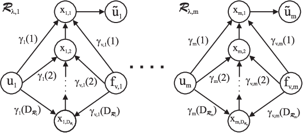
Figure 4 provides an example of the graph representation of $\mathcal{R}_{\lambda}$ when a failure in the node $v$ occurs. The $\gamma$’s labeling some edges of $E_{\mathcal{R}_{\lambda}}$ just indicate that such edges are present if and only if the corresponding $\gamma$’s are not equal to 0. Note that $(V_{\mathcal{R}_{\lambda}},E_{\mathcal{R}_{\lambda}})$ is composed by $m$ weakly connected components, each associated to the data flow of the $i$-th input component. Also note that each node $x_{i,d}$ is a variable associated to the $i$-th input component that will be delivered with a delay $d$ to the actuator node $v_{u,i}$. Finally, note that the sets of input and output nodes are respectively $U\doteq\{u_{1},\ldots,u_{m}\}$ and $\tilde{U}\doteq\{\tilde{u}_{1},\ldots,\tilde{u}_{m}\}$.

The same holds for defining the structured graph representation $(V_{\mathcal{O}_{\lambda}},E_{\mathcal{O}_{\lambda}})$ of block $\mathcal{O}$, where the sets of input and output nodes are respectively $\tilde{Y}\doteq\{\tilde{y}_{1},\ldots,\tilde{y}_{\ell}\}$ and $Y\doteq\{y_{1},\ldots,y_{\ell}\}$.

Finally, let $(V_{\mathcal{P}_{\lambda}},E_{\mathcal{P}_{\lambda}})$ be the structured graph representation of the plant $\mathcal{P}$, where the sets of input and output nodes are respectively $\tilde{U}\doteq\{\tilde{u}_{1},\ldots,\tilde{u}_{m}\}$ and $\tilde{Y}\doteq\{\tilde{y}_{1},\ldots,\tilde{y}_{\ell}\}$.

The model of a MCN $\mathcal{M}$ is the cascade of the blocks $\mathcal{R}$, $\mathcal{P}$ and $\mathcal{O}$. As a consequence, its structured graph representation $(V_{\mathcal{M}_{\lambda}},E_{\mathcal{M}_{\lambda}})$ is given by the union of the structured graph representations of $\mathcal{R}_{\lambda}$, $\mathcal{P}_{\lambda}$ and $\mathcal{O}_{\lambda}$, and the set of nodes $\tilde{U}$ and $\tilde{Y}$ represent the interconnection nodes among such graphs. It is easy to see that all nodes in $\tilde{U}$ and $\tilde{Y}$ are (weak) bridges of $(V_{\mathcal{M}_{\lambda}},E_{\mathcal{M}_{\lambda}})$ since the removal of one of them increases the number of weakly connected components.

In other words, when a failure on a node $v$ occurs, it equally affects all the input components routed via $v$. This assumption is satisfied when $f_{v}(k)$ models a node failure, or when the malicious attack is not able to access separately the input components. We will discuss the case when this assumption does not hold in Section VI.

Let a structured system $S_{\lambda}$ be given in the form:

where $d(k)$ is a vector of disturbance signals and $f(k)=[f_{1}(k),\ldots,f_{r}(k)]^{\top}$ is a vector of $r$ failure signals. In this paper we will not consider the disturbance (i.e. $E_{1}=E_{2}=\boldsymbol{0}$) and leave such generalization to further work. In [3] necessary and sufficient conditions have been derived on the graph representation of $S_{\lambda}$ that (generically) guarantee the existence of a bank of Luenberger observers, which takes as inputs $u(k),y(k)$, generates as output the residual signals vector $\hat{f}(k)=[\hat{f}_{1}(k),\ldots,\hat{f}_{r}(k)]^{\top}$ and is characterized by a transfer function

where $\forall i\in\boldsymbol{r}$, $T_{ii}(z)\neq 0$. Characterizing the existence of such bank of observers is called the bank of observer-based diagonal FDI problem. It is well known that the control input effects can be taken into account in the observer structure, therefore we will consider without loss of generality $B=D=0$. The theorem below characterizes the bank of observer-based diagonal FDI problem when there are no disturbances, and is a particular case of Theorem 3 in [3].

Given a MCN $\mathcal{M}$ subject to failures on communication nodes, if the bank of observer-based diagonal FDI problem is generically solvable for node failures in $\mathcal{M}_{\lambda}$, then the residual signals can be used to detect and identify possibly simultaneous occurrence of node failures. In [21] we proved that, given a MIMO MCN $\mathcal{M}$ and if the plant $\mathcal{P}$ is controllable and observable, it is always possible to design a weight function $W$ such that $\mathcal{M}$ is controllable and observable. As a consequence, we assume in this paper that $\mathcal{M}_{\lambda}$ always satisfies Condition $(i)$ of Theorem 2.

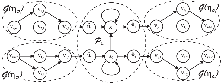
In order to design the network configuration of a MCN $\mathcal{M}$ to enable FDI of node failures, as the main result of this paper we state a formal relation between the network topology $G$ and scheduling/routing $\eta$ of $\mathcal{M}$, and solvability conditions of the bank of observer-based diagonal FDI problem for node failures. With this aim we first propose an algorithm to construct a graph $(\mathcal{V},\mathcal{E})$, which essentially consists of the disjoint union of the controllability and observability graphs associated to each schedule, and of the structured graph representation of the plant. Then we will state a formal relation between solvability conditions of the bank of observer-based diagonal FDI problem for $\mathcal{M}_{\lambda}$ and $(\mathcal{V},\mathcal{E})$.

The following corollary provides necessary and sufficient conditions on network topology, scheduling and routing for FDI of node failures over a MIMO MCN.

Example 2 shows that our results, for small graphs, can be used to enable FDI by manual designing the graph topology, scheduling and routing over the graph $(\mathcal{V},\mathcal{E})$. For more complex networks graph theory algorithms can be exploited to automate the network design process, by searching for disjoint paths for any tentative set of faulty nodes in $2^{|V_{\mathcal{R}}|\cup|V_{\mathcal{O}}|}$, which is characterized by an exponential complexity. In the following we provide a sufficient condition that is easier to be verified.

References

- [1] M. Andersson, D. Henriksson, A. Cervin, and K. Arzen. Simulation of Wireless Networked Control Systems. In Proceedings of the 44th IEEE Conference on Decision and Control and European Control Conference. CDC-ECC 2005, pages 476 – 481, December 2005.
- [2] K. Aström and B. Wittenmark. Computer-Controlled Systems: Theory and Design. Prentice Hall, 1997.
- [3] C. Commault, J.-M. Dion, O. Sename, and R. Motyeian. Observer-based fault detection and isolation for structured systems. IEEE Transactions on Automatic Control, 47(12):2074–2079, December 2002.
- [4] C. Commault and J.-M. Dion. Sensor Location for Diagnosis in Linear Systems: A Structural Analysis. IEEE Transactions on Automatic Control, 52(2):155–169, February 2007.
- [5] A. D’Innocenzo, M.D. Di Benedetto, and E. Serra. Fault tolerant control of multi-hop control networks. IEEE Transactions on Automatic Control, 58(6):1377–1389, June 2013.
- [6] A. D’Innocenzo, G. Weiss, R. Alur, A.J. Isaksson, K.H. Johansson, and G.J. Pappas. Scalable Scheduling Algorithms for Wireless Networked Control Systems. In Proceedings of the 5th IEEE Conference on Automation Science and Engineering (CASE), pages 409–414, 2009.
- [7] R.A. Gupta and M.-Y. Chow. Networked Control System: Overview and Research Trends. IEEE Transactions on Industrial Electronics, 57(7):2527 –2535, July 2010.
- [8] V. Gupta, A.F. Dana, J.P. Hespanha, R.M. Murray, and B. Hassibi. Data transmission over networks for estimation and control. IEEE Transactions on Automatic Control, 54(8):1807–1819, 2009.
- [9] J.-M. Dion, C. Commault, and J. van der Woude. Generic Properties and Control of Linear Structured Systems: a Survey. Automatica, 39(7):1125 –1144, July 2003.
- [10] J.P. Hespanha, P. Naghshtabrizi, and Y. Xu. A Survey of Recent Results in Networked Control Systems. Proceedings of the IEEE, 95(1):138–162, January 2007.
- [11] K.-E. Årzén, A. Bicchi, S. Hailes, K. H. Johansson, and J. Lygeros. On the design and control of wireless networked embedded systems. In Proceedings of the 2006 IEEE Conference on Computer Aided Control Systems Design, Munich, Germany, pages 440–445, October 2006.
- [12] M.-A. Massoumnia, G.C. Verghese, and A.S. Willsky. Failure Detection and Identification. IEEE Transactions on Automatic Control, 34(3):316 –321, March 1989.
- [13] M. Pajic, S. Sundaram, G.J. Pappas, and R. Mangharam. Topological conditions for wireless control networks. In Proceedings of the 50th IEEE Conference on Decision and Control and European Control Conference, Orlando, FL, pages 2353–2360, December 2011.
- [14] M.C.F. Donkers, W.P.M.H. Heemels, N. van de Wouw, and L. Hetel. Stability Analysis of Networked Control Systems Using a Switched Linear Systems Approach. IEEE Transactions on Automatic Control, 56(9):2101 –2115, September 2011.
- [15] M.D. Di Benedetto, A. D’Innocenzo, and E. Serra. Fault Tolerant Stabilizability of Multi-Hop Control Networks. In Proceedings of the 18th IFAC World Congress, Milan, Italy, pages 79–84, 2011.
- [16] J. Neander, T. Lennvall, and M. Gidlund. Prolonging wireless hart network lifetime using packet aggregation. In Proceedings of the IEEE International Symposium on Industrial Electronics (ISIE11), ABB Corp. Res., Bangalore, India, June 27-30, 2011, pages 1230–1236, 2011.
- [17] F. Pasqualetti, A. Bicchi, and F. Bullo. Consensus computation in unreliable networks: A system theoretic approach. IEEE Transactions on Automatic Control, 57(1):90–104, 2012.
- [18] R. Alur, A. D’Innocenzo, K.H. Johansson, G.J. Pappas, and G. Weiss. Modeling and Analysis of Multi-Hop Control Networks. In Proceedings of the 15th IEEE Real-Time and Embedded Technology and Applications Symposium (RTAS), pages 223–232, 2009.
- [19] R. Alur, A. D’Innocenzo, K.H. Johansson, G.J. Pappas, and G. Weiss. Compositional Modeling and Analysis of Multi-Hop Control Networks. IEEE Transactions on Automatic Control, Special Issue on Wireless Sensor and Actuator Networks, 56(10):2345–2357, 2011.
- [20] S. Sundaram, M. Pajic, C.N. Hadjicostis, R. Mangharam, and G.J. Pappas. The Wireless Control Network: Monitoring for Malicious Behavior. In Proceedings of the 49th IEEE Conference on Decision and Control (CDC), pages 5979–5984, December 2010.
- [21] F. Smarra, A. D’Innocenzo, and M.D. Di Benedetto. Fault Tolerant Stabilizability of MIMO Multi-Hop Control Networks. In Proceedings of the IFAC Workshop on Estimation and Control of Networked Systems (NecSys’12), Santa Barbara, CA, pages 79–84, September 14-15 2012.
- [22] F. Smarra, A. D’Innocenzo, and M.D. Di Benedetto. Optimal co-design of control, scheduling and routing in multi-hop control networks. In Proc. of IEEE Conf. on Decision and Control, Maui, Hawaii, pages 1960 – 1965, December 10-13 2012.
- [23] S. Sundaram and C.N. Hadjicostis. Distributed function calculation via linear iterative strategies in the presence of malicious agents. IEEE Trans. on Automatic Control, 56(7):1495–1508, July 2011.
- [24] M. Tabbara, D. Nešić, and A.R. Teel. Stability of Wireless and Wireline Networked Control Systems. IEEE Transactions on Automatic Control, 52(7):1615–1630, September 2007.
- [25] W. Zhang, M.S. Branicky, and S.M. Phillips. Stability of Networked Control Systems. IEEE Control Systems Magazine, 21(1):84–99, February 2001.
- [26] D. B. West. Introduction to Graph Theory. Prentice-Hall Inc., Upper Saddle River, New Jersey, 2001.