Theory of intersecting loops on a torus

We will identify loops (closed paths) on the torus $\mathbb{T}^{2}=\mathbb{R}^{2}/\mathbb{Z}^{2}$ with paths on its covering space ${\mathbb{R}}^{2}$, i.e. we represent all loops on the torus by PL paths on ${\mathbb{R}}^{2}$ between integer points $(m,n)\in\mathbb{Z}^{2}$. All these integer points are identified, and correspond to the same point on the torus. A path in ${\mathbb{R}}^{2}$ representing a loop on the torus can therefore be replaced by any parallel path starting at a different integer point, e.g. the path from $O=(0,0)$ to $(1,1)$ represents the same loop as the path from $(2,0)$ to $(3,1)$, as shown in Figure 1.

A natural subclass of paths in ${\mathbb{R}}^{2}$ are those straight paths denoted $p=(m,n)$ that start at the origin $O=(0,0)$ and end at an integer point $(m,n)\in\mathbb{Z}^{2}$. They generalise the cycles $\gamma_{1},\,\gamma_{2}$ (corresponding to the paths $(1,0)$ and $(0,1)$ respectively). When the path $(m,n)$ is a multiple of another integer path, i.e. $(m,n)=c(m^{\prime},n^{\prime})$, where $m,n,c,m^{\prime},n^{\prime}$ are all integers, with $c\geq 2$, we say it is reducible. Otherwise it is irreducible.

The identification between loops on the torus $\mathbb{T}^{2}=\mathbb{R}^{2}/\mathbb{Z}^{2}$ and PL paths in $\mathbb{R}^{2}$ can be further understood by considering the concept of fundamental reduction. In [15] we introduced this concept in order to better study the intersections between paths $p_{1}$ and $p_{2}$. It consists of reducing one or more paths to a fundamental domain of $\mathbb{R}^{2}$, namely the unit square with vertices $(0,0),(1,0)$ and $(1,1),(0,1)$, as follows: a path that passes through more than one cell (a unit square in $\mathbb{R}^{2}$) consists of ordered segments, each of which passes through only one cell. The fundamental reduction is obtained by superimposing each of these cells, in the order of the segments, on the fundamental domain (the square, or cell, with vertices $(0,0),(1,0)$ and $(1,1),(0,1)$). In this fundamental domain the left and right edges should be identified, and similarly for the top and bottom edges.

Two examples of fundamental reduction for straight paths are shown in Figures 2 and 3. Figure 2 shows a straight path in the first quadrant, namely the path $(2,1)$, with its two segments labelled $s_{1}$ and $s_{2}$ (in that order), and its reduction to the fundamental domain, whereas Figure 3 shows a straight path in the second quadrant, namely $(-1,2)$, and its two segments $s_{1}$ and $s_{2}$ (in that order). Note that, when fundamentally reduced, this path starts at $(1,0)$ (not the origin $O=(0,0)$) and ends at $(0,1)$. This is because its first cell does not coincide with the fundamental domain, and the same is true for non–reduced paths which start in all quadrants except the first.

It is important that in the fundamental domain diagrams (the diagrams on the right) of Figures 2 and 3 the left and right edges should be identified, and similarly for the top and bottom edges, i.e. these diagrams depict a loop on the torus.

As in (1) a quantum matrix is assigned to any straight path $(m.n)$ by

and this clearly extends straightforwardly to any PL path between integer points by assigning a quantum matrix to each linear segment of the path, as in (5), and multiplying the matrices in the same order as the segments along the path. This prescription obviously coincides with the general relation:

where $P$ denotes path-ordering.

In the covering space ${\mathbb{R}}^{2}$, two homotopic loops on the torus are represented by two PL paths on the plane, $p_{1},\,p_{2}$, with the same integer starting point and the same integer endpoint. It was shown in [15] that the following relationship holds for the respective quantum matrices:

where $S(p_{1},p_{2})$ denotes the signed area enclosed between the paths $p_{1}$ and $p_{2}$. Equation (7) generalises equation (3), for which $S(p_{1},p_{2})$ is the area of the square with vertices $(0,0),\,(0,1),\,(1,0)$ and $(1,1)$, i.e. 1. For the general case, the signed area between two PL paths is defined as follows: for any finite region $R$ enclosed by $p_{1}$ and $p_{2}$, if the boundary of $R$ consists of oriented segments of $p_{1}$ and $p_{2}^{-1}$ (the path $p_{2}$ followed in the opposite direction), and is globally oriented in the positive (anticlockwise), or negative (clockwise) sense, this gives a contribution of $+{\rm area}(R)$ , or $-{\rm area}(R)$ respectively, to the signed sum $S(p_{1},p_{2})$ (otherwise the contribution is zero). See Figure 4.

As remarked in [17], the signed area phases are highly suggestive of an underlying geometry with (abelian) surface transports, together with the more conventional parallel transports along paths - see the discussion on $2$ - dimensional holonomy in [19]. For this we need two Lie groups, $G$ and $E$ (related to each other to form a crossed module of groups), and connection $1$ - and $2$ - forms with values in the Lie algebras of $G$ and $E$ respectively. The $1$ - form connection should obviously be $\hat{A}$, and the natural candidate for the connection $2$ - form is the non-vanishing quantum curvature $2$ - form of $\hat{A}$ (see [17]). Since we are dealing with quantum forms, the geometric theory of [19] cannot be applied directly, but it certainly requires investigation.

When part of the path $p_{2}$ is straight but part of the path $p_{1}$ is V-shaped, it can happen that two oppositely signed single intersections at points $R$ and $S$ occur, as shown in Figure 7. Clearly the contributions from the reroutings at $R$ and $S$ should cancel, since the path $p_{2}$ could be deformed to avoid intersecting with $p_{1}$. However, when analyzing the corresponding reroutings (see Figure 8) it is seen that they have zero relative area phase. Although the intersections have opposite sign, the two rerouting terms cannot cancel, since, in the refined Goldman bracket formula (11), the overall factor on the r.h.s. is $(q-1)+(q^{-1}-1)\neq 0$. An identical argument shows that the cancellation also fails to occur when the two paths are interchanged, i.e. $p_{1}$ is straight and $p_{2}$ is V-shaped. To achieve this cancellation extra rules need to be applied. There may be several ways of addressing this issue - we have chosen one possible approach.

The V-intersection rule is defined as follows.

If the total intersection number $\epsilon(\overline{p_{1}},\overline{p_{2}})$ is positive, an extra factor $q$ should be inserted into the term for the negative rerouting, i.e. the overall factor for that rerouting, $(q^{-1}-1)$, is to be replaced by $q(q^{-1}-1)=-(q-1)$. In this way this contribution will cancel with that of the positive rerouting, since $(q-1)+q(q^{-1}-1)=0$. This can be thought of as replacing $(q^{-1}-1)$ with $-(q-1)$, i.e. changing the ‘incorrect’ location of the negative intersection number in the exponent of $q$ to the ‘correct’ location, i.e. as an overall sign multiplying the positive intersection number.

Similarly, if the total intersection number $\epsilon(\overline{p_{1}},\overline{p_{2}})$ is negative, then an extra factor $q^{-1}$ should be inserted into the term for the ‘incorrect’ positive rerouting, replacing $(q-1)$ with $-(q^{-1}-1)$, or, again, changing the ‘incorrect’ location of the intersection number in the exponent of $q$ to the ‘correct’ location, and changing the overall sign.

If the total intersection number $\epsilon(\overline{p_{1}},\overline{p_{2}})$ is zero, then the contributions must cancel in pairs, and for each pair, either of the $R$ and $S$ reroutings (but only one of them) should be adjusted with the above rules.

As an example, take the $p_{1}$ of Figure 8 to be V-shaped, starting at the origin $(0,0)$, passing through the point $(1,-2)$, and ending at $(2,1)$ (i.e. $p_{1}$ is homotopic to the straight path $(2,1)$), whereas $p_{2}$ is straight, $p_{2}=(3,1)$ (see the left figure in Figure 9). Their total intersection number $\epsilon(\overline{p_{1}},\overline{p_{2}})$ is $-1$, which would correspond to a single intersection at the origin if the paths were straight. Because $p_{1}$ is crooked, extra artificial intersections appear, e.g. parallel translating $p_{2}$ to start at $(0,-1)$ we get intersections at $R$ (intersection number $+1$) and at $S$ (intersection number $-1$), giving rise to two rerouted paths which both end at the point $(5,2)$. They are shown in Figure 9. Because the overall intersection number is negative, the $R$ rerouting term should be adjusted with an extra factor $q^{-1}$.

Explicitly, applying the refined formula (11) in this example gives

where the dots indicate the remaining positive rerouting terms and all the negative rerouting terms. Indeed the first two terms on the r.h.s. cancel as they should, due to the extra factor $q^{-1}$ in the first term coming from the V-intersection rule.

Intersections at points where one or both paths change direction precisely at those points are ambiguous, since there is no longer a well-defined tangent direction at the intersection point for one or both paths - see the three examples on the left in Figure 10. This may also occur when the intersection point is the origin, and the direction of the path at its endpoint does not coincide with its direction at the starting point, i.e. the origin (an example is the intersection at the origin of the paths in Figure 9 of Section 4.1, another example will be discussed in Example 1, Section 4.4). The regularization rule consists in replacing the point where the path (or paths) changes direction with a small line segment, extending a distance $\epsilon$ to either side of the point, and adjusting the directions of the incoming and outgoing segments slightly in accordance with this replacement - see the three examples of regularization on the right in Figure 10. Note that the third example in Figure 10 is unlike the other two in that the original, single intersection is replaced by two intersections, with opposite intersection number. An example of this type is the intersection point $U$ of Example 1, Section 4.4 where we will show that the two rerouting terms that arise cancel due to the V-intersection rule.

The direction of the small line segment, or segments, should be chosen so that the intersection with the other path is transversal. The effect of the insertion of $\epsilon$ segments is to remove the ambiguity at the intersection points. After analyzing the intersections and reroutings using the regularized paths, the answer is given by the limit $\epsilon\rightarrow 0$.

An example of this rule is as follows: take $p_{1}$ to be the crooked path $p_{1}=(1,2)S(-1,0)$ (obtained by rerouting the straight path $(1,2)$ along the straight path $(-1,0)$ at the intersection point $S$ as shown on the r.h.s. of Figure 11), i.e. $p_{1}$ is homotopic to $(0,2)$, and take $p_{2}$ to be the straight path $p_{2}=(3,2)$. The overall intersection number is $\epsilon(\overline{p_{1}},p_{2})=-6$, and corresponds to 6 integer starting points for parallel-translated copies of $p_{2}$ in the straight - straight pre - parallelogram, i.e. that formed by $\overline{p_{1}}=(0,2)$ and $\overline{p_{2}}=p_{2}=(3,2)$ (not shown), namely with vertices at $-\overline{p_{2}}$, $-\overline{p_{2}}+\overline{p_{1}}$, $\overline{p_{1}}$ and the origin $O$.

In Figure 12 two of these integer starting points are indicated by black dots, They are the points $(-1,0)$ and $(-2,0)$, and correspond to intersections at $R$ and $T$ respectively. At these points $R$ and $T$ the crooked path $p_{1}$ changes direction (see the first example of Figure 10) and also intersects the parallel copies of $p_{2}$ which start at $(-1,0)$ and $(-2,0)$. Therefore $p_{1}$ should be regularized at these intersections. At the remaining four intersection points $p_{1}$ does not change direction so no regularization is needed.

Figure 13 shows the path $p_{1}$ regularized at $R$ and $T$, with small segments of length $\epsilon$ inserted on either side of the intersections, to make them transversal. Figure 14 displays the reroutings $p_{1}Rp_{2}$ and $p_{1}Tp_{2}$ in the limit $\epsilon\rightarrow 0$.

Combining these rerouting terms with the four terms from the other intersections, we find an expression for the (positive rerouting terms of the) commutator of $\hat{T}(p_{1})$ and $\hat{T}(p_{2})$ that is consistent with the commutator of $\hat{T}(\overline{p_{1}})$ and $\hat{T}(\overline{p_{2}})=\hat{T}(p_{2})$. We illustrate this statement in the case of the intersection point $R$. The commutators should be equal, i.e.

since the relative area phase between $p_{1}$ and $\overline{p_{1}}=(0,2)$ is clearly zero from Figure 11. From the regularization rule as applied in Figure 13, the intersection number $\epsilon(p_{1},p_{2},R)$ is $-1$ which coincides with $\epsilon(\overline{p_{1}},p_{2},R^{\prime})$, where $R^{\prime}$ is the intersection point corresponding to the integer starting point $(-1,0)$ in the pre - parallelogram. The rerouting $\overline{p_{1}}R^{\prime}p_{2}$ is shown in Figure 15. We check that the positive rerouting terms in (11), corresponding to $R$ and $R^{\prime}$ respectively, are in agreement with (15), i.e. equal. Indeed, as shown in Figure 16, the relative area phase for these two reroutings is zero, since the sum of the horizontally shaded areas is clearly equal to the vertically shaded area.

Therefore

A similar reasoning applies to the intersection point $T$ and to the remaining four intersection points which need no regularization.

The final rule, called the missing rule, occurs if we parallel-translate $p_{2}$ to start at an integer point $\beta^{\prime}$ inside the pre - parallelogram for the straightened paths $\overline{p_{1}}$ and $\overline{p_{2}}$, and then find that it does not intersect (i.e. misses) the first path $p_{1}$. An example is shown in Figure 17, where $p_{1}$ is straight and $p_{2}$ is crooked. Note that although $p_{2}$ is V–shaped the missing rule rule should not be confused with the V–intersection rule, which concerns the cancelling of reroutings from pairs of oppositely-signed intersections. Translating $p_{2}$ to start at the integer point $\beta^{\prime}$, lying inside the pre - parallelogram for the straightened paths $\overline{p_{1}}=p_{1}$ and $\overline{p_{2}}$ (dotted lines), it does not intersect $p_{1}$. Hence the usual analysis of intersections and reroutings does not apply. In such circumstances we apply a ‘missing rule’, i.e. add an integer multiple of $\overline{p_{1}}$ to $\beta^{\prime}$ to get a new integer starting point $\beta$, outside the pre - parallelogram, such that the parallel-translated copy of $p_{2}$ starting at $\beta$ does intersect $p_{1}$. In Figure 17 this is achieved by choosing $\beta=\beta^{\prime}+p_{1}$. The resulting intersection point is denoted by $R$.

In such cases the term corresponding to the rerouting of $p_{1}$ along $p_{2}$ at the intersection point $R$ is given an adjustment factor:

to compensate for the fact that its area phase relative to the “normal” rerouted paths has been altered, where “normal” refers to those rerouted paths which arise from a parallel copy of $p_{2}$ with starting point inside the straight - straight pre - parallelogram.

For example, consider the two paths $p_{1}=(-1,0)$ (straight) and $p_{2}=(1,3)P(2,1)$, a crooked path obtained by rerouting $(1,3)$ along $(2,1)$ at the intersection point $P$ - see Figure 18.

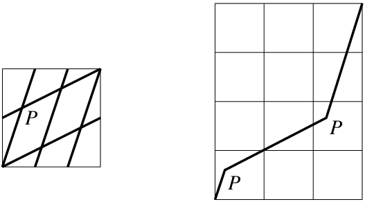
The straightened path $\overline{p_{2}}$ is $(3,4)$ and the total intersection number between $p_{1}$ and $p_{2}$ is $\det(p_{1},\overline{p_{2}})=-4$. Figure 19 shows the straight - straight pre - parallelogram (namely that with clockwise vertices $-\overline{p_{2}}$, $-\overline{p_{2}}+\overline{p_{1}}$, $\overline{p_{1}}$ and the origin $O=(0,0)$). There are four integer starting points, namely the origin $O=(0,0)=\beta^{\prime}_{O}$, $\beta^{\prime}_{1}=(-1,-1)$, $\beta^{\prime}_{2}=(-2,-2)$ and $\beta^{\prime}_{3}=(-3,-3)$.

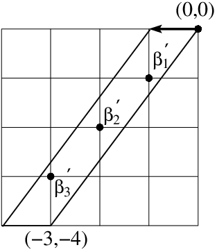
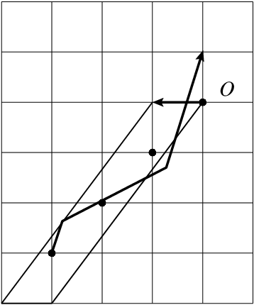
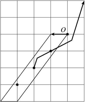
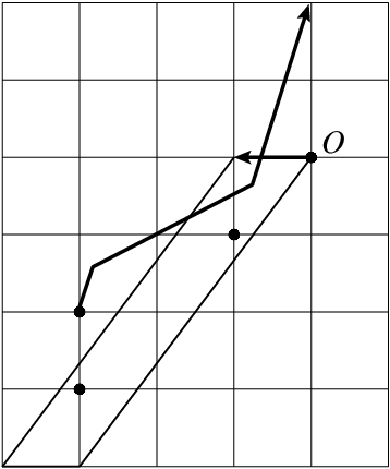
Parallel translating $p_{2}$ to start at these integer points we find that in three cases, namely starting points $O=\beta^{\prime}_{O}$, $\beta^{\prime}_{1}$ and $\beta^{\prime}_{3}$, we get an intersection with $p_{1}$. See for instance the figure on the left of Figure 20 for the starting point $\beta^{\prime}_{3}$ - the other two starting points have the same property. However in one case, namely starting point $\beta^{\prime}_{2}=(-2,-2)$, there is no intersection between the parallel-translated copy of $p_{2}$ starting at $\beta^{\prime}_{2}$ and $p_{1}$ (see the central figure of Figure 20). Applying the missing rule we take the new starting point to be $\beta_{2}=(-3,-2)=p_{1}+\beta^{\prime}_{2}$, as shown in the r.h.s. figure of Figure 20, and compensate by multiplying the corresponding rerouting by the factor (17) where $\beta^{\prime}_{2}-\beta_{2}=-p_{1}=(1,0)$ and $\overline{p_{2}}=(3,4)$, i.e. $\det(\beta^{\prime}_{2}-\beta_{2},\overline{p_{2}})=4$, and the compensating factor is $q^{4}$.

We now illustrate how the missing rule gives a result consistent with the straight - straight result for this example. The area phase for $p_{2}$ relative to $\overline{p_{2}}$ is

as may be seen by using as an intermediary the polygonal path $p_{3}$ going in straight segments from $(0,0)$ to $(1,3)$ to $(3,4)$:

where we used Pick’s formula (13) in the second equation. Then we can use the unrefined formula (10) to calculate the commutator:

We show how one can recover the positive rerouting term in (18) from the refined formula (11) together with the missing rule:

In the first equality of (19) we have used the signed area equation (14) to relate three rerouting terms to the rerouting term at the origin $\hat{T}(p_{1}{O}p_{2})$. The adjustment factor from the missing rule appears as a multiplier in the 3rd term. The passage from $\hat{T}(p_{1}{O}p_{2})$ to $\hat{T}(2,4)$ (the last line of (19)) comes from

where $p_{1}{O}\overline{p_{2}}$ is the polygonal path rerouted at the origin, i.e. straight segments from $(0,0)$ to $(3,4)$ to $(2,4)$, or $\overline{p_{2}}=(3,4)$ followed by $p_{1}=(-1,0)$.

Example 1.

This example requires both the V–intersection rule and the regularization rule. Take $p_{1}$ to be the crooked polygonal line connecting $(0,0)$, $(2,1)$ and $(1,1)$ in that order, and $p_{2}$ to be the straight path $p_{2}=(1,2)$. Their total intersection number is $+1$, although from Figure 21 (the two paths and the reduced paths in a fundamental domain) it appears that there are 6 intersection points. Clearly 5 of these are artificial, since $p_{1}$ is crooked, and their contributions must cancel. This is possible, since after regularization there are six artificial intersection points (see the third example in Figure 10), and they cancel in pairs.

The pair $R$ and $T$ will cancel due to the V–intersection rule, without regularization, and the pair $Q$ and $S$ will cancel, again due to the V–intersection rule, but after regularization. The intersection point $U$ is a case where the regularization rule must be applied as in the third example of Figure 10. After regularization, there are actually two intersection points, denoted $U_{1}$ and $U_{2}$, between the regularized path $p_{1}$ and $p_{2}$, and the corresponding rerouting terms cancel when applying the V-intersection rule, The remaining intersection at $P$ must be regularized. We now proceed to analyse these statements in more detail.

The pair $R$ and $T$ - the intersection points $R$ (intersection number $+1$) and $T$ (intersection number $-1$) form a pair since one can consider them as arising artificially from shifting $p_{2}$ to start at the point $(1,0)$, and end at the point $(2,2)$, as shown on the left in Figure 22. There we have also displayed the corresponding reroutings $p_{1}Rp_{2}$ and $p_{1}Tp_{2}$, and clearly they have relative signed area, namely zero, with respect to each other, or equivalently, they have the same relative signed area, namely $2$, with respect to the straight reference path with endpoint at $(2,3)$.

The V-intersection rule must be applied to $\hat{T}(p_{1}Tp_{2})$, giving an extra factor $q$, since it has the wrong sign with respect to the total intersection number. The two terms corresponding to $R$ and $T$ in the refined bracket $[\hat{T}(p_{1}),\hat{T}(p_{2})]$ then indeed cancel,

The $P$ intersection at the origin is an intersection point, but $p_{1}$ changes direction there since the directions at its starting and endpoints do not coincide: the tangent vector at its starting point is $(2,1)$ and at its endpoint the tangent vector is $(-1,0)$. It should be regularized. We therefore insert a small line segment in the path $p_{1}$ at the origin, and look at the intersections - see Figure 23. The four dots are integer starting points for the parallel-translated copies of $p_{2}$. The origin is the starting point for the intersection at $P$ (and is also $P$ itself), $(1,0)$ is the starting point for the intersections at $R$ and $T$, $(0,-1)$ is the starting point for the intersection at $Q$, and $(1,1)$ is the starting point for the intersection at $S$.

The $Q$ and $S$ intersections also cancel, in the limit $\epsilon\rightarrow 0$. This should be clear from Figure 24, where again we invoke the V-intersection rule.

The intersection at $U$ is more subtle since the path $p_{1}$ also changes direction there (see Figure 21), so we should apply the regularization rule. It is shown in Figure 23 that this leads to two intersections, denoted $U_{1}$ and $U_{2}$, with opposite intersection numbers. When applying the V-intersection rule, the corresponding reroutings (not shown) cancel, since they are equal apart from the intersection number factor and the adjustment factor which comes from applying the V-intersection rule.

Thus the refined bracket $[\hat{T}(p_{1}),\hat{T}(p_{2})]$ gives just one remaining term (for the positive rerouting terms) namely $\hat{T}(p_{1}Pp_{2})$, shown in Figure 25. This is correct, since the relative signed area compared to the rerouted path which would have arisen if we had used $\overline{p_{1}}=(1,1)$ and $p_{2}$, also shown in Figure 25, is exactly the same as the relative signed area relating $p_{1}$ and the straightened $\overline{p_{1}}$ (namely $q^{1/2}$ in both cases). In summary, the refined bracket calculation for this example gives:

after the cancelling of six terms, which is consistent with the straight path result:

since $\hat{T}(\overline{p_{1}})=q^{1/2}\hat{T}(p_{1})$.

This example requires both the regularization rule and the missing rule Take $p_{1}$ to be $p_{1}=(2,1)$, i.e. straight, and $p_{2}$ the crooked polygonal path from $(0,0)$ to $(-2,1)$ to $(-1,2)$. Their total intersection number is $+5$.

Figure 26 shows the paths $p_{1}$ and ${p_{2}}$ (crooked) and their $5$ intersection points, $P^{\prime}$, $Q^{\prime}$,$R^{\prime}$, $S^{\prime}$, and $T^{\prime}$, found by reducing to a fundamental domain. The intersection points $P^{\prime}$ and $S^{\prime}$ are both indicated at the bottom left-hand corner, since they both occur at the starting point of $p_{1}$ (but at two different points of $p_{2}$ - see Figures 29 and 30 where the parallel transported copies of $p_{2}$ are displayed).

Figure 27 shows the five positive reroutings which arise from these intersections.

Figure 28 shows the pre - parallelogram for $p_{1}$ and the straightened path $\overline{p_{2}}=(-1,2)$. The $5$ intersection points, $P$, $Q$, $R$, $S$, and $T$, correspond to 5 integer starting points for parallel translated copies of $\overline{p_{2}}$ (parallel transported to start at integer points inside the pre - parallelogram.)

We now analyse the intersections between $p_{1}$ and ${p_{2}}$ using parallel - translated copies of ${p_{2}}$ starting at different integer points.

For three of the intersections, namely $P^{\prime}$, $R^{\prime}$ and $T^{\prime}$, the integer starting points coincide with starting points in the straight - straight pre - parallelogram of Figure 28, and $R^{\prime}$ and $T^{\prime}$ are transversal intersection points. However $p_{2}$ has a different direction departing from and arrriving at the intersection point $P^{\prime}$, so there the regularization rule needs to be applied - see Figure 29.

For the intersection $S^{\prime}$, the integer starting point also coincides with a starting point in the straight - straight pre - parallelogram of Figure 28, but the intersection with $p_{1}$ is no longer transversal. This is because $S^{\prime}$ is at the vertex of $p_{2}$, i.e. where $p_{2}$ changes direction. Therefore the tangent direction of $p_{2}$, and also the intersection number, are not well-defined there (see Figure 30). Again the regularization rule should be applied, as is done in that Figure.

The intersection point $Q^{\prime}$ is an instance where we must apply the missing rule, since when $p_{2}$ is parallel-translated to the fifth integer point in the straight - straight pre - parallelogram of Figure 28, it fails to intersect $p_{1}$.

Figure 30 shows the situation for the $S^{\prime}$ and $Q^{\prime}$ intersections, displaying the regularization of the copy of $p_{2}$ for $S^{\prime}$ and the integer starting point outside the straight - straight pre - parallelogram for $Q^{\prime}$. The adjustment factor that must be applied to the corresponding rerouting term because of the missing rule (the $Q^{\prime}$ intersection) is given by (17) with $\beta^{\prime}-\beta=-p_{1}=(-2,1)$ and $\overline{p_{2}}=(-1,2)$, i.e. $\det(\beta^{\prime}-\beta,\overline{p_{2}})=-5$, i.e. the compensating factor is $q^{-5}$.

Finally we show part of the calculation which confirms that the application of these rules is consistent with the straight - straight result for this example. The area phase for $p_{2}$ relative to $\overline{p_{2}}$ is

where we used Pick’s formula (13) in the second equality. Then we use the unrefined formula (10) to calculate the commutator:

In (20) the positive rerouting term i.e. $(q-q^{-4})\hat{T}(1,3)$ can be recovered from the refined formula (11), after applying both the regularization rule and missing rules:

In (21) the $5$ terms corresponding to positive reroutings at the points $P^{\prime}$, $R^{\prime}$, $T^{\prime}$, $S^{\prime}$, and $Q^{\prime}$, are given in that order. $\beta_{R^{\prime}},\beta_{T^{\prime}},\beta_{S^{\prime}},\beta_{Q^{\prime}}$ denote the integer starting points of the corresponding rerouted paths (the $P^{\prime}$ rerouting is at the origin) i.e. $\beta_{R^{\prime}}=(1,0)$, $\beta_{T^{\prime}}=(2,0)$, $\beta_{S^{\prime}}=(2,-1)$, $\beta_{Q^{\prime}}=(3,0)$ (see Figures (29) and (30)).

In the first equality of (21) the signed area equation (14), was used to relate four rerouting terms, corresponding to $R^{\prime},T^{\prime},S^{\prime}$ and $Q^{\prime}$, to the first rerouting term at the origin $P^{\prime}=O$, i.e. $\hat{T}(p_{1}{O}p_{2})$. The regularization rule as in Figure 30 justifies the intersection number $(q-1)$ for the rerouting term corresponding to $S^{\prime}$, so that it indeed has the same intersection number as the other intersection points. The adjustment factor from the missing rule appears as the multiplier $q^{-5}$ in the 5th term corresponding to $Q^{\prime}$. The passage from $\hat{T}(p_{1}{O}p_{2})$ to $\hat{T}(3,1)$ in the last line comes from applying Pick’s rule to the rerouting at the origin (the first diagram in Figure 27).

References

- [1] Achúcarro A. and Townsend P.K.,A Chern-Simons Action for Three-Dimensional anti-De Sitter Supergravity Theories, Phys. Lett. B180 (1986) 89.
- [2] Witten E., 2+1 dimensional gravity as an exactly soluble system, Nucl. Phys. B 311 (1998) 46.
- [3] Nelson J. E. and Regge T., Quantum Gravity, Phys. Lett. B 272 (1991) 213.
- [4] Nelson J. E., Regge T. and Zertuche F., Homotopy Groups and dimensional Quantum De Sitter Gravity, Nucl. Phys. B 339 (1990) 516.
- [5] Goldman W. M., Invariant functions on Lie groups and Hamiltonian flows of surface group representations, Invent. Math. 85 (1986) 263.
- [6] Chekhov L.O. and Fock V.V., Observables in 3D Gravity and Geodesic Algebras, Czech. J. Phys. 50 (2000) 1201-1208.
- [7] Penner R.C., The decorated Teichmüller space of punctured surfaces, Commun. Math. Phys. 113 (1987) 299-339.
- [8] Fock V.V., Combinatorial description of the moduli space of projective structures, hepth/9312193.
- [9] Chekhov L., Nelson J. E. and Regge T., Extension of geodesic algebras to continuous genus, Lett.Math.Phys. 78 1, (2006) 17-26.
- [10] Fock V. V.and Rosly A. A., Poisson structure on moduli of flat connections on Riemann surfaces and r-matrix, Am. Math. Soc. Transl., 191 (1999) 67–86.
- [11] Alekseev A.Yu., Grosse H. and Schomerus V., Combinatorial Quantization of the Hamiltonian Chern-Simons theory II, Commun.Math.Phys.174 (1995) 561-604.
- [12] Buffenoir E., Noui K., and Roche P., Hamiltonian quantization of Chern Simons theory with group, Class. Qu. Grav. 19 (2002) 4953–5015.
- [13] Nelson J. E. and Picken R. F., Quantum holonomies in -dimensional gravity Phys. Lett. B 471 (2000) 367.
- [14] Nelson J. E. and Picken R. F., Quantum matrix pairs, Lett. Math. Phys. 52 (2000) 277.
- [15] Nelson J. E. and Picken R. F., Constant connections, quantum holonomies and the Goldman bracket, Adv. Theor. Math. Phys. 9 3 (2005) 407.
- [16] Nelson J. E. and Picken R. F., A quantum Goldman bracket in 2+1 quantum gravity, J. Phys. A: Math. Theor. 41 No 30 (1 August 2008) 304011.
- [17] Nelson J. E. and Picken R. F., Quantum geometry from 2 + 1 AdS quantum gravity on the torus, Gen. Rel. Grav. 43 (2011) 777-795.
- [18] Mikovic A. and Picken R. F. Super Chern-Simons theory and flat super connections on a torus, Adv. Theor. Math. Phys. 5 (2001) 243-63.
- [19] Faria Martins J. and Picken R. F., On 2-Dimensional Holonomy, Trans. Amer. Math. Soc. 362 (2010) 5657-5695.
- [20] Pick G. A., Geometrical aspects of number theory. (Geometrisches zur Zahlenlehre), Sitzenber. Lotos (Prague) 19 (1899) 311: Coxeter H. S. M., Introduction to Geometry 2nd ed. (New York: Wiley) (1969) 209.
- [21] Turaev V. G., Skein quantisation of Poisson algebras of loops on surfaces, Ann. Sci. École Norm. Sup. (4) 24 6 (1991) 635.
- [22] Gukov S., Three-Dimensional Quantum Gravity, Chern-Simons Theory, and the A-Polynomial, Commun.Math.Phys. 255 (2005) 577-627.
- [23] Connes A., Noncommutative Geometry (San Diego, CA: Academic Press) (1994).
- [24] Vaz C. and Witten L., Wilson Loops and Black Holes in 2+1 Dimensions, Phys.Lett. B 327 (1994) 29.