Continuum limit in matrix models for quantum gravity from the Functional Renormalization Group

In the following, we will focus on the matrix model with a $\phi^{4}$ interaction, corresponding to a ”squarulation” of the surface. The continuum limit is universal and independent of the choice of polygons used to construct the discrete simplicial geometry. The additional $Z_{2}$ symmetry of this model restricts the operators that are generated by the Renormalization Group flow. To derive the $\beta$ functions for the hermitian matrix model, it has been suggested in [18] to explicitly integrate out the $(N+1)$th row and column in the path-integral over $(N+1)\times(N+1)$ matrices. Let us briefly review the technique and the results of [18, 33], see also [20, 21]. We consider the action

$$S_{N+1}[\phi_{N+1}]=(N+1){\rm Tr}\left(\frac{\phi_{N+1}^{2}}{2}+\frac{g_{4}}{4}\phi_{N+1}^{4}+\frac{g_{6}}{6}\phi_{N+1}^{6}\right),$$

(9)

which has a $Z_{2}$ symmetry under $\phi_{N+1}\rightarrow-\phi_{N+1}$. We then parameterize the matrix $\phi_{N+1}$ by the matrix $\phi_{N}$ and a complex $N$-component vector $v$ for the $(N+1)$th column and its complex conjugate $v^{\ast}$ for the $(N+1)$th row. The last diagonal entry in $\phi_{N+1}$ is denoted by a complex number $\alpha$. We now explicitly integrate out the vector $v$ in the path integral, which yields an effective action for $\phi_{N}$. In this step, we will only perform the Gaußian integral over $v$, and neglect $\alpha$, which is appropriate in the large-$N$ limit. Re-exponentiating the determinant, and expanding the logarithm, we obtain

	$\displaystyle S^{\prime}[\phi_{N}]$	$\displaystyle=$	$\displaystyle(N+1){\rm Tr}\left(\frac{1}{2}\phi_{N}^{2}+\frac{g_{4}}{4}\phi_{N}^{4}+\frac{g_{6}}{6}\phi_{N}^{6}\right)$		(10)
		$\displaystyle+$	$\displaystyle g\,{\rm Tr}\left(\phi_{N}^{2}\right)-\frac{g_{4}^{2}}{2}{\rm Tr}\left(\phi_{N}^{4}\right)+g_{6}{\rm Tr}\left(\phi_{N}^{4}\right).$

In order to recover the canonical normalization of the quadratic term in $\phi_{N}$, we perform a rescaling

$$\phi_{N}=\rho\phi_{N}^{\prime},$$

(11)

with

$$\rho=1-\frac{2g_{4}+1}{2N}+\mathcal{O}\left(\frac{1}{N^{2}}\right).$$

(12)

It is then straightforward to read off the relation between the couplings $g_{4}^{\prime}$ and $g_{4}$

$$\frac{N\,g_{4}^{\prime}}{4}=(N+1)\frac{g_{4}}{4}\rho^{4}.$$

(13)

With the definition

$$g_{4}-g_{4}^{\prime}=\frac{1}{N}\beta(g)$$

(14)

we then obtain the following $\beta$ functions, where terms $\mathcal{O}\left(\frac{1}{N}\right)$ are neglected:

	$\displaystyle\beta_{g_{4}}$	$\displaystyle=$	$\displaystyle g_{4}+6g_{4}^{2}+4g_{6},$
	$\displaystyle\beta_{g_{6}}$	$\displaystyle=$	$\displaystyle-g_{6}\left(1-3(1+2g_{4})\right)+6g_{4}g_{6}-6g_{4}^{3}.$		(15)

For $g_{6}=0$ this is the result obtained in [18] (note that our definition of the $\beta$ function differs by a sign) and extended to higher order in the couplings and to include further couplings in [33]. We obtain

$$g_{4\,\ast}=-0.1057,\quad g_{6\,\ast}=-0.0097.$$

(16)

For the critical exponents¹¹ 1 These determine whether a coupling must be tuned in order to reach a particular fixed point: From Eq.(20) we can deduce the solution to the linearized flow around the fixed point $$\beta_{g_{i}}(\{g_{n}\})=\sum_{j}\frac{\partial\beta_{g_{i}}}{\partial g_{j}}\Big|_{g_{n}=g_{n\,\ast}}\left(g_{j}-g_{j\,\ast}\right)+\mathcal{O}((g_{j}-g_{j\,\ast})^{2})\,.$$ (17) The solution to this linearized equation reads $$g_{i}(N)=g_{i\,\ast}+\sum_{I}C_{I}V^{I}_{i}\left(\frac{N}{N_{0}}\right)^{-\theta_{I}},$$ (18) where $$-\frac{\partial\beta_{g_{i}}}{\partial g_{j}}\Big|_{g_{n}=g_{n\,\ast}}V_{I}=\theta_{I}V_{I}.$$ (19) Herein, $C_{I}$ is a constant of integration and $N_{0}$ is a reference ”scale”. The $V_{I}$ are the eigenvectors and $-\theta_{I}$ the eigenvalues of the stability matrix, which is defined by Eq.(17). The additional negative sign in $\theta_{I}$ is useful, because then $\theta_{I}$ equals the canonical dimensionality at a non-interacting fixed point. In order to approach the fixed point in the IR, observe that the $C_{I}$ are arbitrary for irrelevant directions where $\theta_{I}<0$. In contrast, a relevant direction with $\theta_{I}>0$ corresponds to a parameter that needs to be tuned in order to ensure that the fixed point is reached in the IR., generally defined by

$$\theta_{i}=-{\rm eig}\left(\frac{\partial\beta_{g_{i}}}{\partial g_{j}}\right)\Big|_{g_{k}=g_{k\,\ast}},$$

(20)

we obtain

$$\theta_{1}=1,\quad\theta_{2}=-1.46.$$

(21)

Let us discuss the significance of this result: As expected, the fixed point has one relevant direction, as only $g_{4}$ needs to be tuned in the double-scaling limit. We observe that $g_{6}$, although itself an irrelevant coupling, yields a significant contribution to $\beta_{g_{4}}$, and improves $g_{4\,\ast}$ from the value $-1/6$ which is the fixed-point value for $g_{6}=0$.

The exact value $g_{c}=-1/12$ is approximated by our result, and at a first glance, the value of $\theta$ does not seem to be too different from the exact value $\theta=-0.8$. In fact, this value can be traced to the ”canonical dimensionality” of the coupling, which yields the term $\sim g$ in the $\beta$ function: In order to obtain a nontrivial fixed point in

$$\beta_{g}=g(1+c\,g),$$

(22)

where $c$ is a constant, $g_{\ast}=-\frac{1}{c}$. Then,

$$\theta=-\partial_{g}\beta_{g}|_{g=g_{\ast}}=-(1+c\,g_{\ast})-g_{\ast}c=1.$$

(23)

Accordingly we observe that at this order, the value of the critical exponent is determined by the dimensionality, and does not depend on the fixed-point value at all.

In the following, we will introduce a method that generalizes the idea to integrate out matrix entries, such that it applies beyond the perturbative regime, and can be generalized directly to higher-dimensional tensor models. We will set up a nonperturbative Renormalization Group equation that allows to determine the scaling of couplings with the matrix size $N$.

To that end, let us first introduce the notion of scaling dimensionality in these models.

As this model does not have a natural notion of momentum – it can be viewed as a zero-dimensional field theory in this sense – there is no standard canonical dimensionality of the couplings. Spacetime, and the attribution of momentum dimensions as familiar from high-energy physics, only emerges in the continuum limit. Nevertheless, couplings have an inherent dimensionality that determines their behavior under rescalings in $N$, just as the canonical dimensionality in standard quantum field theories determines the canonical scaling under standard scale-transformations. From the expression Eq.(15), one can distinguish two types of contributions to the $\beta$ function: There are contributions proportional to one power of the coupling itself, or higher powers of the coupling and higher-order couplings. The same structure appears in $\beta$ functions in high-energy physics. There it is clear that a loop-diagram that yields the contribution of quantum fluctuations to the $\beta$ function of $g_{i}$ cannot be proportional to one power of $g_{i}$ only. Instead it arises from the canonical dimensionality (and is therefore absent, e.g., in QCD in $d=4$.) In the same way, this type of contribution reflects the scaling dimensionality of the matrix model couplings under a rescaling in $N$.

The canonical scaling dimensionality of the couplings is determined in the following way: Considering only single-trace terms, the action can be written as

$$\bar{S}=\frac{Z_{\phi}}{2}{\rm Tr}\left(\phi^{2}\right)+\sum_{i}\bar{g}_{i}{\rm Tr}\left(\phi^{i}\right),$$

(24)

where $Z_{\phi}$ is a wavefunction renormalization. In order to establish the contact to the generating functional for 2d quantum gravity, a rescaling of the fields $\phi\rightarrow\sqrt{N}\phi$ and couplings is useful, such that

$$S=N\left(\frac{Z_{\phi}}{2}{\rm Tr}\left(\phi^{2}\right)+\sum_{i}\tilde{g}_{i}{\rm Tr}\left(\phi^{i}\right)\right),$$

(25)

as then each Feynmandiagram is weighted by a factor $N^{\chi}$, where $\chi$ is the Euler character of the surface associated to the diagram. This holds, as in the above parameterization, each vertex contributes a factor $N$, each propagator a $N^{-1}$ and each face, i.e., each closed loop, $N$ due to the associated index summation. Thus each diagram contributes with $N^{V-E+F}$, where $V,E$ and $F$ count the number of vertices, edges and faces, respectively. As $V-E+F=\chi$, the identification $N=e^{\gamma}$ then allows to make contact with the generating functional for 2d quantum gravity, cf. Eq.(1). We therefore read off the following relation between $\tilde{g}_{i}$ and $\bar{g}_{i}$:

$$\bar{g}_{i}N^{\frac{i-2}{2}}=\tilde{g}_{i}.$$

(26)

This analysis agrees with the corresponding terms in the perturbative $\beta$ function in [18, 33], cf. Eq.(15).

We observe that even the coupling with the lowest number of fields, $g_{4}$, is power-counting irrelevant, as it has dimensionality $-1$. We conclude that quantum fluctuations will be responsible for a shift towards relevance at the fixed point corresponding to the double-scaling limit.

To assign canonical dimensionality to terms with several traces, such as $\bar{g}_{i,j}{\rm Tr}\phi^{i}\,{\rm Tr}\phi^{j}$, we demand that each additional trace should be suppressed by a factor $\frac{1}{N}$. This assignment cancels the additional factor of $N$ that is associated with the additional trace.

Accordingly this yields

$$\bar{g}_{i,j}N^{\frac{i+j}{2}}=\tilde{g}_{i,j}.$$

(27)

At the same order in $\phi$, a double-trace term accordingly is shifted by one into irrelevance in comparison to the corresponding single-trace operator. This is consistent with the expectation that only one coupling should be tuned in the double-scaling limit. For the single trace operators, the coupling $g_{4}$ of dimensionality $-1$ is shifted into relevance, but not the coupling $g_{6}$ of dimensionality $-2$, cf. Eq.(21). The assignment of dimensionality $-2$ to the first two-trace-operator $({\rm Tr}\phi^{2})^{2}$ already suggests that it will not be shifted into relevance, if we assume that the contribution of quantum fluctuations to the scaling of different operators is of similar size.

If we further rescale the kinetic term to its canonical coefficient $1/2$, the renormalized dimensionless couplings $g_{i}$ are then given by

$$g_{i}=\frac{\tilde{g}_{i}}{Z_{\phi}^{i/2}}=\frac{\bar{g}_{i}N^{\frac{i-2}{2}}}{Z_{\phi}^{i/2}},\quad g_{i,j}=\frac{\bar{g}_{i,j}N^{\frac{i+j}{2}}}{Z_{\phi}^{\frac{i+j}{2}}}.$$

(28)

Accordingly, the $\beta$ functions will take the following form

$$\beta_{g_{i}}=\frac{i-2}{2}g_{i}+\frac{i}{2}\eta g_{i}+\dots,$$

(29)

where $\eta=-\partial_{t}\ln Z_{\phi}$ and further terms are induced by quantum fluctuations. This form agrees with the $\beta$ functions that can be derived by explicit integration over matrix entries, cf. [18, 33]. Let us now introduce a novel tool to perform this integration and derive the nonperturbative form of the $\beta$ functions.

At this point is is useful to comment on the universality of the fixed-point values: As is well-known, for a dimensionless coupling, the one-loop and two-loop coefficients of the $\beta$ function are universal, but higher orders are not. For dimensionful couplings, such as all couplings in our case, even the one-loop coefficient is nonuniversal. This implies that fixed-point values will not be universal, either. In contrast, the critical exponents are universal. Accordingly a comparison of $g_{\ast}$ to $g_{c}$ is less meaningful than the comparison of the critical exponents with the exact result.

To generalize the perturbative setting of integrating over matrix entries, we use the framework of the nonperturbative functional Renormalization Group, [34], for reviews see [35, 36, 37, 38, 39, 40, 41, 42].

Our approach here is closely related to similar developments in [43], where the functional Renormalization Group was used to demonstrate the property of asymptotic safety in the Grosse-Wulkenhaar model [44, 45]. A main difference to the present setting is the absence of a nontrivial kinetic term in our case, and the implications for the canonical dimensionality and the implementation of the matrix cutoff in the following. Note that this approach crucially differs from former applications of the functional Renormalization Group to matrix models in the context of condensed-matter models, see, e.g., [35]: There, quantum fluctuations of matrix-valued fields that are function on spacetime, are integrated out according to their momentum.

To derive the change of the generating functional under an integration of matrix entries between $N$ and $N+\delta N$, we follow the usual steps in setting up a flowing effective action: We consider the generating functional $\mathcal{Z}=\int_{\Lambda}d\phi e^{-S[\phi]+J\cdot\phi}$, where $\Lambda$ is a UV cutoff on $N$ and $J$ is a source. We then define an $N$-dependent generating functional, where $N$ will be an infrared cutoff on the matrix size, i.e., we will integrate out matrix entries above $N$, but not below. We introduce a ”mass-like” regulator function

$$\Delta S_{N}[\phi]=\frac{1}{2}\phi_{ab}R_{N}(a,b)_{ab\,cd}\phi_{cd},$$

(30)

where we now explicitly indicate the matrix indices $a,b,\dots$ for clarity. The function $R_{N}(a,b)$ can have any form compatible with the following three requirements:

	$\displaystyle\underset{a/N\rightarrow 0,c/N\rightarrow 0}{\rm lim}R_{N}(a,b)_{ab\,cd}$	$\displaystyle>$	$\displaystyle 0,$		(31)
	$\displaystyle\underset{N/a\rightarrow 0,N/a\rightarrow 0}{\rm lim}R_{N}(a,b)_{ab\,cd}$	$\displaystyle=$	$\displaystyle 0$		(32)
	$\displaystyle\underset{N\rightarrow\Lambda\rightarrow\infty}{\rm lim}R_{N}(a,b)_{ab\,cd}$	$\displaystyle\rightarrow$	$\displaystyle\infty.$		(33)

Introducing this mass-type term into the generating functional

$$\mathcal{Z}_{N}=\int_{\Lambda}d\phi\,e^{-S[\phi]-\Delta S_{N}[\phi]+J\cdot\phi},$$

(34)

yields a suppression of the matrix entries in the block $a,b=1,\dots,N$, cf. Eq.(31). In contrast, the ”UV” matrix entries with indices $a,b>N$ are integrated out. Thus the generating functional $\mathcal{Z}_{N}$ contains the effect of ”UV” quantum fluctuations above $N$. Taking the limit $N\rightarrow 0$, the suppression term should approach zero, such that all matrix entries are integrated out in this limit, cf. Eq.(32). This is a direct generalization of the idea put forward in [18] to integrate the $(N+1)$th row and column of the matrices explicitly.

We now define an $N$ dependent flowing action by a modified Legendre transform

$$\Gamma_{N}[\varphi]=\underset{J}{\rm{sup}}\left(J\varphi-\ln\mathcal{Z}_{N}\right)-\Delta S_{N}[\varphi].$$

(35)

The divergence of $\Delta S_{N}$ for $N\rightarrow\Lambda\rightarrow\infty$, cf. Eq.(33), ensures that $\Gamma_{N\rightarrow\Lambda}\simeq S_{\rm bare}$, as it enforces a saddle-point evaluation of the path-integral. For $N\rightarrow 0$, $\Gamma_{N}\rightarrow\Gamma$, which is the full effective action and contains the effect of all quantum fluctuations.

It is now straightforward to derive an equation encoding the change of $\Gamma_{N}$ under a change of $N$, which is the Wetterich equation for the matrix model case:

$$\partial_{t}\Gamma_{N}=\frac{1}{2}{\textrm{tr}}\left(\Gamma_{N}^{(2)}+R_{N}\right)^{-1}\partial_{t}R_{N},$$

(36)

where $t=\ln N$. $\Gamma_{N}^{(2)}$ denotes the second functional derivative with respect to the degrees of freedom, in this case the entries of matrices. $\left(\Gamma_{N}^{(2)}+R_{N}\right)^{-1}$ is nothing but the regularized, nonperturbative field-dependent propagator of the theory. Accordingly the operator trace tr in the Wetterich equation yields a one-loop form, cf. fig. 1. It is important to realize that the derivation of the Wetterich equation does not rely on the existence of a small parameter. It is therefore applicable in the nonperturbative regime. As a technical advantage, it takes a one-loop form, while the presence of the full propagator includes nonperturbative effects in this setting.

In order to obtain the $\beta$ function of a particular coupling, it is necessary to project the flowing action onto that coupling, by taking appropriate derivatives with respect to $\phi$. If the same projection prescription is applied to the Wetterich equation, this yields the $\beta$ function of the corresponding coupling. Diagrammatically, the derivatives with respect to $\phi$ generate vertices with a coupling to an external $\phi$, as $\frac{\partial}{\partial\phi}\left(\Gamma_{N}^{(2)}\right)^{-1}=-\left(\Gamma_{N}^{(2)}\right)^{-1}\left(\frac{\partial}{\partial\phi}\Gamma_{N}^{(2)}\right)\left(\Gamma_{N}^{(2)}\right)^{-1}$, cf. fig. 2.

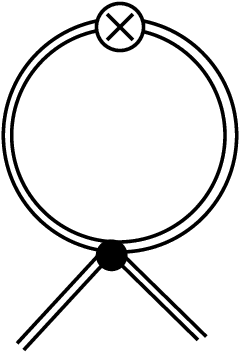
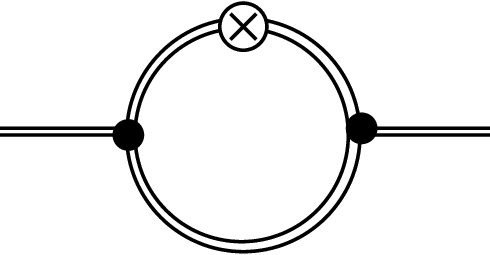
Thus the contributions to the $\beta$ function of a particular coupling with $n$ powers of $\phi$ consist of all one-loop diagrams with $n$ external $\phi$’s and therefore up to $n$ vertices.

The main difference between the matrix model and the usual setting for quantum field theories on a spacetime is the lack of a kinetic operator, and the nonstandard assignment of canonical dimensionality.

As quantum fluctuations generate all operators that are compatible with the symmetries, $\Gamma_{N}$ will contain further operators beyond those in the bare action. We thus have to consider the Renormalization Group flow in the typically infinite-dimensional theory space of all couplings compatible with the symmetries of the model. While the Wetterich equation is exact, in practice its solution requires a truncation of $\Gamma_{N}$, which implies an approximative result. In the present setting, the effective action can be expanded in terms of multiple traces of $\rho=\phi^{2}$, containing operators such as ${\rm Tr}\phi^{n}$ and ${\rm Tr}\phi^{n}{\rm Tr}\phi^{m}$, which yield a basis for theory space. In our case, the $Z_{2}$ symmetry restricts the class of allowed operators to those with even powers in the field. Note that the introduction of the regulator into the generating functional breaks the $U(\Lambda)$ symmetry of the matrix model, as matrix entries below $N$ acquire a mass-type term, while those above $N$ do not. This implies that further terms will be generated that go beyond that theory space, very much in the same way as the flow equation generates, e.g., a gluon mass term in the flow for non-Abelian gauge theories, see, e.g., [38]. Here, we will only consider the flow of operators that are permitted by the original symmetry ²² 2 In principle, the Renormalization Group flow of the hermitian matrix model could be derived after diagonalizing the action. This would however require a technically involved treatment of the Vandermonde determinant, see [11, 15]..

To project onto the couplings of the corresponding operators, we will use the $\mathcal{P}^{-1}\mathcal{F}$ expansion of the flow equation: We split $\Gamma_{N}^{(2)}+R_{N}=\mathcal{P}_{N}+\mathcal{F}_{N}$, where all field-dependent terms enter the fluctuation matrix $\mathcal{F}_{N}$. We can then expand the right-hand side of the flow equation as follows:

	$\displaystyle\partial_{t}\Gamma_{N}$	$\displaystyle=$	$\displaystyle\frac{1}{2}\textrm{tr}\{[\Gamma_{N}^{(2)}+R_{N}]^{-1}(\partial_{t}R_{N})\}$		(37)
		$\displaystyle=$	$\displaystyle\frac{1}{2}\textrm{tr}\,\tilde{\partial}_{t}\ln\mathcal{P}_{N}+\frac{1}{2}\sum_{n=1}^{\infty}\frac{(-1)^{n-1}}{n}\textrm{tr}\,\tilde{\partial}_{t}(\mathcal{P}_{N}^{-1}\mathcal{F}_{N})^{n},$

where the derivative $\tilde{\partial}_{t}$ in the second line by definition acts only on the $N$ dependence of the regulator, $\tilde{\partial}_{t}=\textrm{tr}\partial_{t}R_{N}\frac{\delta}{\delta R_{N}}$. As each power of $\mathcal{F}_{N}$ contains a dependence on the matrix $\phi$, this expansion corresponds to an expansion in the number of vertices. To project, e.g., on the running of $g_{4}$, we need only up to the second order of the $\mathcal{P}^{-1}\mathcal{F}$ expansion, as a tadpole vertex $\sim g_{6}$ and a two-vertex diagram with vertices $\sim g_{4}$ are the only one-loop diagrams that can contribute to the running of the $\phi^{4}$ term. (If our action contained terms $\sim\phi^{3}$, three-vertex and four-vertex diagrams would also contribute.)

We will now explain how to apply this equation in a concrete case, and show that the perturbative results by [18, 33] can be reproduced. As a first step, we use that any hermitian matrix $\phi$ can be decomposed into a real symmetric matrix $A$ and a real antisymmetric matrix $B$ by

$$\phi_{ab}=A_{ab}+i\,B_{ab},$$

(38)

and decompose all terms ${\rm tr}\phi^{n}$ accordingly. For the projection onto the invariants ${\rm tr}\phi^{i}\,\dots{\rm tr}\phi^{j}$ we can then use diagonal matrices of the form

$$A_{ij}=a\delta_{ij}.$$

(39)

Different orders in $\phi$ are then distinguished by powers of $a$. Operators with the same number of fields but different numbers of traces are distinguished by powers of $N$. $\Gamma^{(2)}$ then takes the form of a matrix in field space, with entries $\Gamma^{(2)}_{AA}$, $\Gamma^{(2)}_{AB}$, $\Gamma^{(2)}_{BA}$ and $\Gamma^{(2)}_{BB}$, where we can set $B=0$ after taking the derivative. The inverse propagator matrix then takes a very simple form: Due to the antisymmetry, any term with an odd number of $B$’s vanishes. The two off-diagonal terms $\Gamma^{(2)}_{AB}$ and $\Gamma^{(2)}_{AB}$ are also zero, since they contain only terms with odd numbers of $B$s. $\Gamma^{(2)}_{BB}$ is nonzero, but does not contain any powers of $B$. This diagonal structure greatly simplifies the evaluation of the operator trace.

For the derivatives we use that

	$\displaystyle\frac{\delta}{\delta A_{ab}}A_{cd}$	$\displaystyle=$	$\displaystyle\frac{1}{2}\left(\delta_{ad}\delta_{bc}+\delta_{ac}\delta_{bd}\right),$		(40)
	$\displaystyle\frac{\delta}{\delta B_{ab}}B_{cd}$	$\displaystyle=$	$\displaystyle-\frac{1}{2}\left(\delta_{ad}\delta_{bc}-\delta_{ac}\delta_{bd}\right).$		(41)

The propagators for the two matrix modes are then given by

	$\displaystyle P^{-1}_{AA\,abcd}$	$\displaystyle=$	$\displaystyle\frac{1}{Z_{\phi}(1+R_{N}(a,c))}\left(\delta_{ad}\delta_{bc}+\delta_{ac}\delta_{bd}\right),$		(42)
	$\displaystyle P^{-1}_{BB\,abcd}$	$\displaystyle=$	$\displaystyle-\frac{1}{Z_{\phi}(1+R_{N}(a,c))}\left(\delta_{ad}\delta_{bc}-\delta_{ac}\delta_{bd}\right),$		(43)

where $Z_{\phi}$ is a wave function renormalization.

It is important to realize that the derivative of ${\rm tr}\phi^{n}$ generates two very different types of terms, only one of which generates nonzero contributions to $\beta_{g_{i}}$: As an example, consider

			$\displaystyle\frac{\delta}{\delta A_{ab}}\frac{\delta}{\delta A_{cd}}\frac{\bar{g}_{4}}{4}{\rm Tr}A^{4}$		(45)
		$\displaystyle=$	$\displaystyle\frac{\bar{g}_{4}}{2}\Bigl(A_{cn}A_{na}\delta_{bd}+A_{cn}A_{nb}\delta_{ad}+A_{dn}A_{na}\delta_{bc}+A_{dn}A_{nb}\delta_{ac}$
			$\displaystyle+A_{bd}A_{ca}+A_{bc}A_{da}\Bigr),$

where we use a summation convention for indices that occur twice.

Contracting this expression with the propagator and taking the operator trace, there will be a term $\sim\delta_{aa}$ and a term that does not involve a Kronecker-delta anymore:

			$\displaystyle{\rm{tr}}P^{-1}_{AA\,abcd}\left(\frac{\delta}{\delta A_{ab}}\frac{\delta}{\delta A_{cd}}\frac{\bar{g}_{4}}{4}{\rm Tr}A^{4}\right)$		(46)
		$\displaystyle=$	$\displaystyle\bar{g}_{4}\frac{1}{Z_{\phi}(1+R_{N}(a,b))}A_{an}A_{na}\delta_{bb}$
			$\displaystyle+\bar{g}_{4}\frac{1}{Z_{\phi}(1+R_{N}(a,a))}A_{an}A_{na}$
			$\displaystyle+\frac{\bar{g}_{4}}{2}\frac{1}{Z_{\phi}(1+R_{N}(a,b))}A_{ab}A_{ba}$
			$\displaystyle+\frac{\bar{g}_{4}}{2}\frac{1}{Z_{\phi}(1+R_{N}(a,b))}A_{aa}A_{bb}$

The terms which are generated correspond to ${\rm Tr}\left(\phi^{2}\right)$ and $\left({\rm Tr}\left(\phi\right)\right)^{2}$, since these are the only two terms at $\mathcal{O}(\phi^{2})$. The two terms can be clearly distinguished above: The first term will be $\sim{\rm Tr}\,\phi^{2}$, as will be the second and third term. The fourth one is clearly $\sim\left({\rm Tr}\left(\phi\right)\right)^{2}$. Inserting our choice of projection Eq.(39) after this identification, we obtain a scaling $\sim N^{2}$ for the first term and a scaling $\sim N$ for the second and third, and $\sim N^{2}$ for the fourth one. Going over to the dimensionless coupling $g_{4}$, each term receives an additional power of $N^{-1}$. To project onto the dimensionless coupling of ${\rm Tr}\left(\phi^{2}\right)$, we require a scaling $\sim N$. Therefore, only the first term will yield a contribution at $\mathcal{O}(N^{0})$, whereas the second and third one will be suppressed by $\frac{1}{N}$. To project onto the dimensionful coupling of $\left({\rm Tr}\left(\phi\right)\right)^{2}$, we require a scaling $\sim N$, since the coupling has dimensionality $-1$, and a factor $N^{2}$ arises from the two traces. Thus the third term gives a $\mathcal{O}(N^{0})$ contribution to the flow of this coupling.

We use a regulator that is inspired by Litim’s optimized cutoff [46] and takes the form

$$R_{N}(a,b)_{abcd}=Z_{\phi}P_{A/B\,abcd}\left(\frac{2N}{a+b}-1\right)\theta\left(1-\frac{a+b}{2N}\right),$$

(47)

where $P_{A\,abcd}=\frac{1}{2}\left(\delta_{ad}\delta_{bc}+\delta_{ac}\delta_{bd}\right)$ for the $A$ mode and $P_{B\,abcd}=-\frac{1}{2}\left(\delta_{ad}\delta_{bc}-\delta_{ac}\delta_{bd}\right)$ for the $B$ mode. The factor of 2 in the argument of the shape function accounts for the fact that both matrix indices $a,b$ will run up to $N$. Here one can observe a major difference to settings with a non-trivial kinetic term, where the corresponding operator would multiply the shape function on the RHS of Eq.(47) to define the regulator. We then have that

			$\displaystyle\partial_{t}R_{N}(a,b)_{abcd}$		(48)
		$\displaystyle=$	$\displaystyle P_{A/B\,abcd}\Bigl[\left(\partial_{t}Z_{\phi}\left(\frac{2N}{a+b}-1\right)+Z_{\phi}\frac{2N}{a+b}\right)\theta\left(1-\frac{a+b}{2N}\right)$
			$\displaystyle+Z_{\phi}\left(\frac{2N}{a+b}-1\right)\delta\left(1-\frac{a+b}{2N}\right)\frac{a+b}{2N}\Bigr],$

where the $\delta$ distribution in the second line does not contribute to sums/integrals over $a,b$ due to the factor in front. For this choice of cutoff we have that

$$\sum_{a}\sum_{b}\left(P^{-1}_{a\,b}\right)^{n}\partial_{t}R_{N}\sim N^{2}\frac{4\left(2+n-\eta\right)}{2+3n+n^{2}}\left(1+\mathcal{O}(1/N)\right).$$

(49)

Here we have approximated the sum by an integral, which is correct at leading order in $\frac{1}{N}$. We are now in a position to derive the $\beta$ functions with the Wetterich equation.

Let us first analyze a simple truncation of the effective action, which reads

$$\Gamma_{N}=\frac{Z_{\phi}}{2}{\rm Tr}\left(\phi^{2}\right)+\frac{\bar{g}_{4}}{4}{\rm Tr}\left(\phi^{4}\right)+\frac{\bar{g}_{6}}{6}{\rm Tr}\left(\phi^{6}\right).$$

(50)

Using the methods outlined above, we can derive a set of $\beta$ functions, which read

	$\displaystyle\eta$	$\displaystyle:=$	$\displaystyle-\partial_{t}\ln Z_{\phi}=2g_{4}\frac{1}{3}\left(4-\eta\right),$		(51)
	$\displaystyle\beta_{g}$	$\displaystyle=$	$\displaystyle g_{4}+2\eta g_{4}+4g_{4}^{2}\frac{1}{5}\left(5-\eta\right)-4g_{6}\frac{1}{3}\left(4-\eta\right),$		(52)
	$\displaystyle\beta_{g_{6}}$	$\displaystyle=$	$\displaystyle 2g_{6}+3\eta g_{6}+12g_{4}\,g_{6}\frac{1}{5}\left(5-\eta\right)-6g_{4}^{3}\frac{2}{15}\left(6-\eta\right),$

where the factors of $\eta$ on the right-hand side arise from the use of an RG-adjusted regulator, i.e., $R_{N}\sim Z_{\phi}$, and accordingly $\partial_{t}R_{N}\sim\eta+\dots...$ Diagrammatically, the flow equation for these $\beta$ functions is shown in fig. 2 and fig. 3. Similar diagrams with 6 external matrices yield the flow of $g_{6}$.

The anomalous dimension clearly depends on the coupling in a nonperturbative way, as the solution of Eq.(51) reads

$$\eta=\frac{8g_{4}}{3+2g_{4}}.$$

(54)

We find, apart from the Gaußian fixed point, the fixed point corresponding to the double-scaling limit at

$$g_{4\,\ast}=-0.072,\quad g_{6\,\ast}=-0.004.$$

(55)

The critical exponents, defined by

$$\theta_{I}=-{\rm eig}\left(\frac{\partial\beta_{g_{i}}}{\partial g_{j}}\right)\Big|_{g_{k}=g_{k\,\ast}},$$

(56)

are given by

$$\theta_{1}=1.046,\quad\theta_{2}=-1.080.$$

(57)

As expected, we obtain one UV-relevant direction, which corresponds to the coupling that has to be tuned in order to reach the double-scaling limit. The exact results are given by

$$g_{c}=-\frac{1}{12},\quad\theta=-0.8.$$

(58)

To check whether our truncation approaches these exact results, let us consider the smaller truncation with $g_{6}=0$. Then the fixed point value and critical exponent are given by

$$g_{4\,\ast}=-0.101,\,\quad\theta=1.066.$$

(59)

We observe that the full result is approached closer in the larger truncation, as expected. We also observe that the nonperturbative information encoded in the structure of $\eta$ through Eq.(54) leads to a smaller value for $g_{4\,\ast}$ in comparison to the results in [33], where $g_{4\,\ast}=-0.103$, $g_{6\,\ast}=-0.005$.

As a next step, we will include further single-trace operators to study the convergence of the critical exponent under extensions of the truncation.

The single-trace operator truncation, i.e., an ansatz for the effective action of the form

$$\Gamma[\phi]=\textrm{Tr}\,V\left(\phi^{2}\right)=\frac{Z_{\phi}}{2}\textrm{Tr}\left(\phi^{2}\right)+\sum_{n\geq 2}\frac{\bar{g}_{2n}}{2n}\,\textrm{Tr}\left(\phi^{2n}\right),$$

(60)

can be seen as an analogue of the local potential approximation. It shares three features in particular with the local potential approximation: (1) it is a truncation containing an infinite number of couplings $\bar{g}_{2n}$, (2) it contains the interesting couplings $g_{2}=Z_{\phi},\,g_{4}$ and contains the most relevant coupling at each power of $\phi$, as further traces decrease the canonical dimensionality, in the same way that further derivatives in a standard QFT decrease the canonical dimensionality and (3) one can find a closed expression for the beta functions in the limit $N\to\infty$:

$$\eta=g_{4}[\dot{R}P^{2}]$$

(61)

			$\displaystyle\beta_{2n}$
		$\displaystyle=$	$\displaystyle\left((1+\eta)n-1\right)g_{2n}$
		$\displaystyle+$	$\displaystyle\!2n\!\!\!\!\!\!\!\sum_{{{i;\,}}n=\sum_{i}i\,m_{i}}\!\!\!\!\!\!\left(-1\right)^{\sum_{i}\!\!m_{i}}[\dot{R}P^{1+\sum_{i}\!\!m_{i}}]\left(\begin{array}[]{c}\sum_{i}m_{i}\\ m_{1},m_{2},...\end{array}\right)\prod_{i}g_{2(i+1)}^{m_{i}},$

where the $m_{i}$ are positive integers and $\sum_{i}m_{i}$ corresponds to the order of the $\mathcal{P}^{-1}\mathcal{F}$ expansion and denotes the number of vertices in the diagram. By $\dot{R}P^{n}$ we denote $\mathcal{P}^{-n}\partial_{t}R_{N}$. The bracket denotes the multinomial coefficient $\frac{(\sum_{i}m_{i})!}{m_{1}!m_{2}!...}$. This factor arises, as in the $\mathcal{P}^{-1}\mathcal{F}$ expansion to order $n$, a contribution proportional to more than one coupling arises several times. For instance, a contribution $\sim g_{i}g_{j}$, $i\neq j$ comes with a factor of 2, as either one of the factors $\mathcal{F}$ can be either $\sim g_{i}$ or $\sim g_{j}$. In this expression, the factors $\frac{1}{n}$ from the $\mathcal{P}^{-1}\mathcal{F}$ expansion (cf. Eq.(37)) cancel against a factor $n$ when the $\tilde{\partial}_{t}$ derivative acts on $\mathcal{P}^{-n}$. The validity of (II.5) can be seen in a vertex expansion for the single trace truncation (60), which starts with the $\mathcal{F}$-term

$$F^{abcd}=\sum_{n\geq 1}\bar{g}_{2n}\left(\delta_{ac}(\phi^{2})^{n-1}_{db}+...+(\phi^{2})^{n-1}_{ac}\delta_{db}\right),$$

(65)

where the ellipsis denotes the summands without any $\delta$. The contribution of any trace that does not contract a complete sequence of $\delta$’s is suppressed by $1/N$ and is thus suppressed in the limit $N\to\infty$. Consequently, there are only two products in $(F^{n})^{abcd}$ that are not suppressed in the limit $N\to\infty$, namely the one contracting solely over the initial $\delta$ and the one contracting over the final $\delta$. These terms yield the same field monomial and hence produce a factor of $2$ that cancels the $\frac{1}{2}$ from the RHS of the flow equation, cf. Eq.(37). Consequently, equation (61) for $\eta$ follows from the fact that the only summand in (65) that contains at most two fields is the term containing a single $g_{4}$. Moreover, using the reciprocal power series formula

			$\displaystyle\left(1+\sum_{n\geq 1}{{\epsilon}}^{n}g_{n}\right)^{-1}$		(66)
		$\displaystyle=$	$\displaystyle\sum_{n=0}^{\infty}\epsilon^{n}\sum_{n=\sum_{i}im_{i}}(-1)^{\sum_{i}m_{i}}\left(\begin{array}[]{cc}\sum_{i}m_{i}\\ m_{1},m_{2},...\end{array}\right)\prod_{i}g_{i}^{m_{i}},$

and dimensionless couplings $g_{2n}=N^{n-1}Z_{\phi}^{-n}\bar{g}_{2n}$, one finds equation (II.5) directly form the vertex expansion.

Let us use (61) and (II.5) to investigate the effect of increasing the number of single trace operators in the truncation on the numerical values of the non-Gaussian fixed point. The explicit expressions for the first beta functions are

	$\displaystyle\beta_{4}$	$\displaystyle=$	$\displaystyle(1+2\eta)g_{4}+4\left(-[\dot{R}P^{2}]g_{6}+[\dot{R}P^{3}]g_{4}^{2}\right),$		(70)
	$\displaystyle\beta_{6}$	$\displaystyle=$	$\displaystyle(2+3\eta)g_{6}+6\left(-[\dot{R}P^{2}]g_{8}+2[\dot{R}P^{3}]g_{4}g_{6}-[\dot{R}P^{4}]g_{4}^{3}\right),$

	$\displaystyle\beta_{8}$	$\displaystyle=$	$\displaystyle(3+4\eta)g_{8}+8\left(-[\dot{R}P^{2}]g_{10}+[\dot{R}P^{3}](g_{6}^{2}+2g_{8}g_{4})\right.$		(72)
			$\displaystyle\left.-3[\dot{R}P^{4}]g_{4}^{2}g_{6}+[\dot{R}P^{5}]g_{4}^{4}\right),$
	$\displaystyle\beta_{10}$	$\displaystyle=$	$\displaystyle(4+5\eta)g_{10}$		(73)
			$\displaystyle+10\left(-[\dot{R}P^{2}]g_{12}+2[\dot{R}P^{3}](g_{4}g_{10}+g_{6}g_{8})\right.$
			$\displaystyle\left.-3[\dot{R}P^{4}](g_{4}^{2}g_{8}+g_{4}g_{6}^{2})+4[\dot{R}P^{5}]g_{4}^{3}g_{6}-[\dot{R}P^{6}]g_{4}^{5}\right),$
	$\displaystyle\beta_{12}$	$\displaystyle=$	$\displaystyle(5+6\eta)g_{12}+12\left(-[\dot{R}P^{2}]g_{14}\right.$		(74)
			$\displaystyle\left.+[\dot{R}P^{3}](2g_{4}g_{12}+2g_{6}g_{10}+g_{8}^{2})\right.$
			$\displaystyle\left.-[\dot{R}P^{4}](g_{6}^{3}+3g_{4}^{2}g_{10}+6g_{4}g_{6}g_{8})\right.$
			$\displaystyle\left.+[\dot{R}P^{5}](6g_{4}^{2}g_{6}^{2}+4g_{4}^{3}g_{8})\right.$
			$\displaystyle\left.-5[\dot{R}P^{6}]g_{4}^{4}g_{6}+[\dot{R}P^{7}]g_{4}^{6}\right),$
	$\displaystyle\beta_{14}$	$\displaystyle=$	$\displaystyle(6+7\eta)g_{14}+14\left(-[\dot{R}P^{2}]g_{16}\right.$		(75)
			$\displaystyle\left.+2[\dot{R}P^{3}](g_{4}g_{14}+g_{6}g_{12}+g_{8}g_{10})\right.$
			$\displaystyle\left.-3[\dot{R}P^{4}](g_{4}^{2}g_{12}+2g_{4}g_{6}g_{10}+g_{4}g_{8}^{2}+g_{6}^{2}g_{8})\right.$
			$\displaystyle\left.+4[\dot{R}P^{5}](g_{4}^{3}g_{10}+3g_{4}^{2}g_{6}g_{8}+g_{4}g_{6}^{3})\right.$
			$\displaystyle\left.-5[\dot{R}P^{6}](g_{4}^{4}g_{8}+2g_{4}^{3}g_{6}^{2})+6[\dot{R}P^{7}]g_{4}^{5}g_{6}-[\dot{R}P^{8}]g_{4}^{7}\right).$

The factors $\dot{R}P^{n}$ are dependent on the choice of regulator and defined by Eq.(49) for our choice of shape function. We find a non-interacting Gaußian fixed point with canonical critical exponents and several interacting fixed points, of which the only one with only one relevant direction is the one of interest for the double-scaling limit. The numerical values $g_{2n}^{*}$ for the couplings at that particular non-Gaussian fixed point and the critical exponents $\theta_{i}$, are given in tab. 1.

It turns out that in each order in the expansion there is only one positive critical exponent, $\theta_{1}$, which means in particular that increasing the truncation does not introduce new relevant directions. We also observe that the irrelevant critical exponents approach the values $\theta_{i}=d_{i}+1$, where $d_{i}$ is the canonical dimensionality of the couplings in the truncation. At the same time, the eigenvectors of the stability matrix do not directly correspond to the couplings $g_{i}$, but to superpositions of them. To increasing order in the truncation, we observe an apparent convergence of the eigenvalues: We observe that the positive critical exponent approaches smaller values. As the difference in the values between subsequent truncation orders becomes smaller in every step, an extrapolation of $\theta$ for truncation order $n\rightarrow\infty$ yields $\theta>1$. We conclude that operators are still missing from this truncation. Very much in analogy to the critical exponents for the Wilson-Fisher fixed point, further operators at each order in the fields are missing: For the Wilson-Fisher fixed point, next-to-next to leading order in the derivative expansion is necessary for accurate critical exponents [47, 48]. In our case, the missing operators at a given power of the fields are multi-trace operators. We will demonstrate how to include these in the following. Let us briefly explain why we take into account operators that are power-counting irrelevant, cf. Eq.(27), and that we expect to remain irrelevant, as the double-scaling limit corresponds to only one relevant direction. At an interacting fixed point, both irrelevant and relevant couplings take non-zero values. Accordingly, nonvanishing contributions from the fluctuation of irrelevant operators couple into the flow of relevant couplings. Thus the fixed-point values and critical exponents of a relevant direction receive nonvanishing contributions from irrelevant couplings. Therefore the (ir) relevance of a coupling is not a criterion to distinguish whether this coupling yields large correction to $\beta$ functions at an interacting fixed point.

References

- [1] J. Ambjorn and J. Jurkiewicz, Phys. Lett. B 278, 42 (1992).
- [2] J. Ambjorn, A. Goerlich, J. Jurkiewicz and R. Loll, Phys. Rept. 519, 127 (2012) [arXiv:1203.3591 [hep-th]].
- [3] J. Ambjorn, S. Jordan, J. Jurkiewicz and R. Loll, Phys. Rev. Lett. 107, 211303 (2011) [arXiv:1108.3932 [hep-th]].
- [4] V. Rivasseau, arXiv:1209.5284 [hep-th].
- [5] V. Rivasseau, AIP Conf. Proc. 1444, 18 (2011) [arXiv:1112.5104 [hep-th]].
- [6] D. V. Boulatov, Mod. Phys. Lett. A 7, 1629 (1992) [hep-th/9202074].
- [7] L. Freidel, Int. J. Theor. Phys. 44, 1769 (2005) [hep-th/0505016].
- [8] D. Oriti, PoS QG -PH, 030 (2007) [arXiv:0710.3276 [gr-qc]].
- [9] D. Oriti, arXiv:1110.5606 [hep-th].
- [10] D. Weingarten, Nucl. Phys. B 210, 229 (1982); F. David, Nucl. Phys. B 257, 45 (1985); Nucl. Phys. B 257, 543 (1985); J. Ambjorn, B. Durhuus and J. Frohlich, Nucl. Phys. B 257, 433 (1985); V. A. Kazakov, A. A. Migdal and I. K. Kostov, Phys. Lett. B 157, 295 (1985); D. V. Boulatov, V. A. Kazakov, A. A. Migdal and I. K. Kostov, Phys. Lett. B 174, 87 (1986); Nucl. Phys. B 275, 641 (1986).
- [11] P. Di Francesco, P. H. Ginsparg and J. Zinn-Justin, Phys. Rept. 254, 1 (1995) [hep-th/9306153].
- [12] M. R. Douglas and S. H. Shenker, Nucl. Phys. B 335, 635 (1990).
- [13] E. Brezin and V. A. Kazakov, Phys. Lett. B 236, 144 (1990).
- [14] D. J. Gross and A. A. Migdal, Phys. Rev. Lett. 64, 127 (1990); Nucl. Phys. B 340, 333 (1990).
- [15] P. H. Ginsparg and G. W. Moore, In *Boulder 1992, Proceedings, Recent directions in particle theory* 277-469. and Yale Univ. New Haven - YCTP-P23-92 (92,rec.Apr.93) 197 p. and Los Alamos Nat. Lab. - LA-UR-92-3479 (92,rec.Apr.93) 197 p [hep-th/9304011].
- [16] J. Ambjorn, hep-th/9411179.
- [17] M. Marino, hep-th/0410165.
- [18] E. Brezin and J. Zinn-Justin, Phys. Lett. B 288, 54 (1992) [hep-th/9206035].
- [19] J. Alfaro and P. H. Damgaard, Phys. Lett. B 289, 342 (1992) [hep-th/9206099].
- [20] S. Higuchi, C. Itoi and N. Sakai, Prog. Theor. Phys. Suppl. 114, 53 (1993) [hep-th/9307154].
- [21] S. Higuchi, C. Itoi, S. Nishigaki and N. Sakai, Nucl. Phys. B 434, 283 (1995) [Erratum-ibid. B 441, 405 (1995)] [hep-th/9409009].
- [22] S. Dasgupta and T. Dasgupta, hep-th/0310106.
- [23] J. Ambjorn, B. Durhuus and T. Jonsson, Mod. Phys. Lett. A 6, 1133 (1991).
- [24] N. Sasakura, Mod. Phys. Lett. A 6, 2613 (1991).
- [25] M. Gross, Nucl. Phys. Proc. Suppl. 25A, 144 (1992).
- [26] R. Gurau, Commun. Math. Phys. 304, 69 (2011) [arXiv:0907.2582 [hep-th]].
- [27] R. Gurau, Annales Henri Poincare 12, 829 (2011) [arXiv:1011.2726 [gr-qc]].
- [28] R. Gurau and V. Rivasseau, Europhys. Lett. 95, 50004 (2011) [arXiv:1101.4182 [gr-qc]].
- [29] R. Gurau, Annales Henri Poincare 13, 399 (2012) [arXiv:1102.5759 [gr-qc]].
- [30] R. Gurau, Phys. Rev. D 84, 124051 (2011) [arXiv:1110.2460 [hep-th]].
- [31] S. Dartois, R. Gurau and V. Rivasseau, arXiv:1307.5281 [hep-th].
- [32] R. Gurau, Class. Quant. Grav. 27, 235023 (2010) [arXiv:1006.0714 [hep-th]].
- [33] C. Ayala, Phys. Lett. B 311, 55 (1993) [hep-th/9304090].
- [34] C. Wetterich, Phys. Lett. B 301, 90 (1993).
- [35] J. Berges, N. Tetradis and C. Wetterich, Phys. Rept. 363 (2002) 223 [hep-ph/0005122].
- [36] J. Polonyi, Central Eur. J. Phys. 1 (2003) 1. [hep-th/0110026].
- [37] J. M. Pawlowski, Annals Phys. 322 (2007) 2831 [arXiv:hep-th/0512261].
- [38] H. Gies, in Renormalization Group and Effective Field Theory Approaches to Many-Body Systems, Lecture Notes in Physics, Vol 852, pp 287-348 (2012) arXiv:hep-ph/0611146.
- [39] B. Delamotte, Lect. Notes Phys. 852, 49 (2012) [cond-mat/0702365 [COND-MAT]].
- [40] O. J. Rosten, arXiv:1003.1366 [hep-th].
- [41] W. Metzner et al., Rev. Mod. Phys. 84, 299 (2012).
- [42] J. Braun, J. Phys. G 39, 033001 (2012) [arXiv:1108.4449 [hep-ph]].
- [43] A. Sfondrini and T. A. Koslowski, Int. J. Mod. Phys. A 26, 4009 (2011) [arXiv:1006.5145 [hep-th]].
- [44] H. Grosse and R. Wulkenhaar, Commun. Math. Phys. 256, 305 (2005) [hep-th/0401128].
- [45] M. Disertori, R. Gurau, J. Magnen and V. Rivasseau, Phys. Lett. B 649, 95 (2007) [hep-th/0612251].
- [46] D. F. Litim, Phys. Rev. D 64, 105007 (2001) [hep-th/0103195].
- [47] L. Canet, B. Delamotte, D. Mouhanna and J. Vidal, Phys. Rev. B 68, 064421 (2003) [hep-th/0302227].
- [48] D. F. Litim and D. Zappala, Phys. Rev. D 83, 085009 (2011) [arXiv:1009.1948 [hep-th]].
- [49] H. Gies, Phys. Rev. D 66, 025006 (2002) [hep-th/0202207].
- [50] D. Benedetti and F. Caravelli, JHEP 1206, 017 (2012) [Erratum-ibid. 1210, 157 (2012)] [arXiv:1204.3541 [hep-th]].
- [51] J. A. Dietz and T. R. Morris, JHEP 1301, 108 (2013) [arXiv:1211.0955 [hep-th]].
- [52] D. F. Litim and J. M. Pawlowski, Nucl. Phys. Proc. Suppl. 74, 325 (1999) [hep-th/9809020].
- [53] D. F. Litim and J. M. Pawlowski, hep-th/9901063.
- [54] J. Ben Geloun and D. O. Samary, Annales Henri Poincare 14, 1599 (2013) [arXiv:1201.0176 [hep-th]].
- [55] J. Ben Geloun, Class. Quant. Grav. 29, 235011 (2012) [arXiv:1205.5513 [hep-th]].
- [56] J. Ben Geloun, arXiv:1210.5490 [hep-th].
- [57] S. Weinberg, In *Hawking, S.W., Israel, W.: General Relativity*, 790-831 (Cambridge University Press, Cambridge, 1980).
- [58] H. Gies and M. M. Scherer, Eur. Phys. J. C 66, 387 (2010) [arXiv:0901.2459 [hep-th]].
- [59] H. Gies, S. Rechenberger, M. M. Scherer and L. Zambelli, arXiv:1306.6508 [hep-th].
- [60] M. Reuter, Phys. Rev. D 57, 971 (1998) [hep-th/9605030].
- [61] M. Reuter and F. Saueressig, New J. Phys. 14, 055022 (2012) [arXiv:1202.2274 [hep-th]].